Abstract
For the structural health diagnostic of concrete dams, the mathematical monitoring model based on the measured deformation values is of great significance. The main purpose of this paper is to reconstruct the ageing component and the temperature component in the traditional Hydraulic-Seasonal-Time (HST) hybrid model by combining the measured values. On the one hand, a better mathematical model for the ageing displacement of concrete dams is proposed combined with the Burgers model to separate the instantaneous elastic hydraulic deformation and the hysteretic hydraulic deformation, and then it subsumes the latter into the ageing deformation to describe its reversible component. According to the Burgers model, the inverted elastic modulus of the Jinping-Ⅰ concrete dam is 46.5 GPa, which is closer to the true value compared with the HST model. On the other hand, the kernel principal component analysis (KPCA) method is used to extract the principal components of the dam thermometers for replacing the period harmonic thermal factor. A multiple linear regression (MLR) model is established to fit the measured displacement of the concrete arch dam and to verify the accuracy of the proposed hybrid model. The results show that the proposed model reaches higher accuracy than the traditional HST hybrid model and is helpful to improve the interpretation of the separated displacement components of the concrete dams.
1. Introduction
Since the increasing requirement and utilization of water resources in China, a large amount of concrete dams have been constructed and contributed significantly to economic development [1,2]. The safety issues and the risks of dam failure are always unavoidable due to uncertainties in geology, hydrology, design, construction, and operational management. The dam failure, which resulted in major casualties, is a tragic lesson worldwide. Hence, dam safety has always been a high priority for governments and relevant authorities and has played an important role in preventing dam failures.
Displacement, stress, strain, and cracks [3,4,5,6,7,8,9] et al. are essential for dam health monitoring and operational instruction. As the most intuitive reflection of the integrity of concrete dams, displacement is frequently adopted for predicting the behaviour of the dam. Among the models that were used to fit and predict dam displacements, there are two main categories. The first one is based on deterministic functions, physical extrapolation methods, and multiple linear regression. For instance, statistical, deterministic, and hybrid models are the commonly used monitoring models in engineering. Chen et al. [10] adopted a semi-parametric statistical model, which has more imitative effect and explanatory than the parametric statistical model. Shang [11] analysed the key dam section of the roller compacted concrete (RCC) gravity dam with statistical modeling methods. Hu et al. [12] proposed a statistical hydrostatic-thermal-crack-time model to deal with the influential horizontal cracks in concrete arch dams. Another type is based on machine learning models. Kang et al. [13] presented a dam health monitoring model based on kernel extreme learning machines. Chen et al. [14] combined the advantages of extreme learning machines and elastic networks for predicting dam deformation. Su et al. [15] used rough set theory and a support vector machine to build the early-warning models of dam safety. The monitoring models based on machine learning techniques; however, do not take the structural characteristics of the concrete dams into account. Furthermore, they lack direct mathematical expressions, causing them to only be useful for making predictions rather than providing a causal interpretation of dam deformation, such as statistical models [16].
The causes of ageing components in dams are complex, including cracking [17], alkali-aggregate reactions (AAR) [18], dissolution [19], etc. It can also be interpreted by the compression deformation of the rock foundation structure, as well as self-generated volume deformation and irreversible displacement due to cracks in the dam. Therefore, the ageing displacement is relatively difficult to give the mathematical expression directly according to the actual situation. Among a variety of HST-based models, the ageing component is expressed as the exponential function or the combination of the linear and logarithmic functions. However, the formation mechanism of the ageing displacement of the concrete dam caused by the theological properties of the dam material is extremely complicated. Therefore, the HST model based on a simple exponential function or a logarithmic function may not appropriately represent the relationships between the influencing factors and the dam displacement. The development law of the ageing component is studied and expressed as some function of time, which can then be separated in some way based on the relationship between the ageing displacement and the dam load to optimize the traditional HST model. For instance, Li et al. presented a hydrostatic-seasonal-state (HSS) model for rationally obtaining and accurately interpreting ageing displacement from total displacement monitoring data [20]. Hu and Wu [12] presented a statistical hydrostatic-thermal-crack-time model and applied it to assess the impact of the large-scale horizontal crack on the Chencun dam’s downstream face. To explain the abnormal displacement behaviour of the Jinping-I arch dam, Wang et al. [21] introduced a hysteretic hydraulic component into the HST model, transforming the traditional HST model into an improved HHST model. The ageing component reflects a combination of reversible and irreversible deformation of the dam body and rock foundation. According to the changing pattern of the displacement and the periodic regulation of the reservoir water level for the concrete dams, Gu and Wu [22] concluded that a combination of the exponential and periodic harmonic functions, which are used for the irreversible and reversible ageing displacements [23], should be used to represent the ageing displacement according to the periodic regulation of the reservoir water level for most dams.
The temperature displacement component is the displacement due to temperature changes in the dam body and rock foundation of the dam; thermometer measurements of the dam body and rock foundation of the dam should be selected as a factor. The traditional hybrid model expressed the temperature component in the statistical mode and then was optimally fitted to the measured values. In recent years, the thermal components have been extracted or considered in dam displacement prediction by various methods [24]. Mata et al. conducted the Short Time Fourier Transform analysis of the residuals to determine the impact of the daily air temperature variation on the displacement of concrete dams [25]. Kang et al. considered that the temperature varies over time and substituted harmonic sinusoidal functions to the long-term air temperature for thermal effect simulation [26]. Chen et al. [27] adopted kernel principle component analysis (KPCA) to extract the temperature variables. Among a significant number of the thermometers buried in the dam sections, principal component extraction is an important process. Additionally, the KPCA method used in the paper (20) validates that it assists to reduce the dimensionality of the thermal measurement results by minimizing the loss of the original information.
The main idea of this paper is to propose a new hybrid model. For the extraction of the ageing component, a better mathematical model for the ageing displacement of concrete dams is proposed. For the temperature component, the KPCA method is used to extract the inherent characteristics of the thermometer measurement data to substitute the periodic harmonic factors. Then, a multiple linear regression (MLR) model is developed to fit the measured displacement to validate the reasonableness of the extracted ageing component and temperature component. In this paper, the MLR model is established based on Matlab. The accuracy of the new hybrid model and the extracted components are compared with the components in the HST model. The displacement components of the concrete dam can be more easily understood with the help of the suggested model.
The research significance is for dam safety based on the monitoring model of displacement messages, which can fully reflect the recoverable creep component of the concrete and rock and accurately separate the ageing component from the total displacement.
2. Model Establishment
The factors influencing dam displacement can be broadly summarized as water level, temperature, and time. The traditional HST hybrid model can be generally interpreted as the following equation:
where δH, δT, and δθ represent the hydraulic displacement component, temperature displacement component, and ageing displacement component, respectively; is the FEM-calculated hydraulic component; X is the adjustment coefficient; H is the water depth of the upstream reservoir on the same monitoring day; t is the number of cumulative days since the initial monitoring day; θ is equal to t/100.
2.1. FEM-Calculated Elastic Hydraulic Component
In the traditional HST hybrid model, the ageing component only contains the irreversible component. The reversible ageing displacement follows the same evolution rule as the instantaneous hydraulic displacement due to the common causal factor of reservoir water pressure, these two types of displacements are separated into the hydraulic component in the paper [28]. In contrast to the instantaneous elastic modulus determined by the material properties, the inverted elastic modulus of dam body concrete provides a thorough reflection of the immediate and hysteretic elastic deformation ability through the analysis of the traditional HST hybrid model [3]. According to the theoretical derivation above, the hysteretic water pressure component is subsumed into the ageing component in this paper; therefore, only the elastic water pressure component needs to be calculated by the finite element method [29] as follows:
where δHe is the actual water pressure component. is the water pressure component value obtained from the elastic finite element calculation; X is the total water pressure component adjustment factor, and E0 is the initial value of the instantaneous elastic modulus used in the calculation.
In the conventional elastic inversion method, the resulting modulus of elasticity of the dam concrete is a composite reflection of the instantaneous elastic deformation and viscoelastic hysteresis deformation. Therefore, a combined model of mechanical elements is required to separate the instantaneous elastic modulus and viscoelastic modulus when calculating the elastic hydrodynamic component. The Burgers model is a four-parameter fluid model that is commonly used to describe viscoelastic behaviour. It is a hybrid of the Maxwell and Kelvin–Voigt models. The Maxwell model is used to describe stress relaxation, but only in the case of irreversible flow. Although the Kelvin–Voigt model can represent creep, it cannot represent instantaneous deformation. It is not able to account for the stress relaxation [28]. After the combination of these two models, the Burgers model can express both relaxation and creep effects after combining these two models [30]. Many researchers have used it extensively in recent years to describe the dynamic behaviour of viscoelastic materials [31,32]. Thus, it is used in this paper to calculate the instantaneous and hysteretic hydraulic displacements by the FEM and in the inversion analysis.
2.2. Mathematical Expression of the Ageing Displacement of the Concrete Dam Considering Viscoelastic Deformation
Dam structural properties primarily consist of three states: elasticity, viscoelasticity, and unstable failure [33]. The dam monitoring displacement consists of two components: an elastic component and a nonlinear component that fluctuates with load and time (commonly known as the time effect). The elastic displacement is influenced and calculated by the instantaneous elastic modulus. The actual ageing displacement is a process of increasing and decreasing around a certain base value, including irrecoverable and recoverable terms [34]. The factors that generally affect the ageing displacement include the material properties of the dam concrete, such as autogenous volume displacement, wet and dry displacement, plastic displacement, creep of concrete, the material properties of the dam base rock, and the creep of the dam structure. Creep deformation reflects an inherent property of the dam concrete and the rock. It consists of an irreversible viscoplastic component and a reversible viscoelastic (also known as hysteretic elastic) component. During a long period of creep displacement, the reversible viscoelastic component accounts for a significant portion of the total elastic displacement [35], which is influenced by the delayed elastic modulus separated by the Burgers model shown in Figure 1. On a macroscopic scale, the displacement is characterised by a high degree of variation at the beginning of the storage period, followed by a gradual stabilisation over time. However, laboratory tests on concrete and rock have shown that a portion of the creep displacement of concrete and rock recovers after the unloading lag. Part of the recovery is influenced by the size of the unloading and the time of unloading, as well as the age of the concrete, as shown in Figure 2.
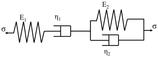
Figure 1.
The Burgers model for dam concrete.
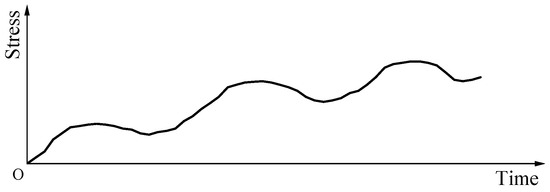
Figure 2.
The radial displacement and the reservoir water level of the NO.9 dam section.
In the case of intermittent loading, the creep is a combination of increasing and decreasing curves. Because the water level in a reservoir is constantly changing, its effect on the dam can be seen as intermittent loading. As the water level is lowered, the dam and rock body thus undergo some non-linear recovery of creep with time, which can be linked to the delayed elastic moduli of the dam concrete. Therefore, it would not be accurate enough to describe the ageing displacement simply as a monotonically increasing function. A new model needs to be investigated to make the fit more accurate. As mentioned above, the ageing displacement is caused by the creep of the concrete and rock foundation and the plastic deformation caused by the compression of fractures and joints in the concrete and rock base. Their effects are discussed separately as follows.
2.2.1. Creeping Law of Concrete
The total strain ε(t) of concrete at age τ1, under the action of the external force σ(τ1) can be expressed by the following equation [36]:
where C(t, τ1) is the creep degree of the concrete; E(τ1) is the modulus of elasticity of concrete at age τ1.
In general, dams are old enough when they are built to hold water. According to the theory of elastic creep, the creep at load changes conforms to the principle of superposition, i.e., [37]:
where is the stress increment at the moment .
The variation pattern of Equation (5) can be seen in Figure 2, which shows the effect of load history on strain.
2.2.2. Derivation of the Equation for the Creep Displacement of a Dam on a Rigid Foundation
Assume that the modulus of elasticity of the foundation Er→∞. The dam is built on a rigid foundation, and the water pressure can be approximated as proportional loading; according to the theory of creep mechanics, the total displacement u at the top of the dam can be expressed as [38]:
where ue is the elastic displacement under external load.
f(t) can be expressed as follows [39]:
For a dam, its physical force is a constant and can be taken as φ(t,τ) = 1. So, the above equation becomes
After deducting the elastic displacement from Equation (6), we can obtain
Substitute Equation (8) into Equation (9) and give
ξ(t,τ,τ1) in Equation (10) is the kernel of integration and using the conclusions of elastic creep theory, can be expressed as [40]:
Substitute ξ(t,τ,τ1) into Equation (10) and give
When taking p = 1, it can be expressed as
It should be noted that in Equation (13), δθ is the creep displacement at time t when the water level is H (the water level at the age of the dam concrete at τ1). In fact, the water level in the reservoir is constantly changing from time τ1 to time t. Therefore, considering the water level change, the displacement expression at the moment t is
where ue(H,t) and ue(H,τ) are the elastic displacements of the dam crest due to the reservoir water pressure at moments t and τ.
The age of the dam concrete is generally large due to reservoir storage. Therefore, it can be assumed that E(t) is a constant. Thus, ue, E(t), and C1 are combined as and E(t) and C2 are combined as . τ1 is the age of the concrete at the start of the monitored displacement. Therefore, τ − t can be replaced by −t′. t′ indicates that the first day of the period starts at zero. In this way, Equation (14) can be rewritten as [38]
2.2.3. Creep Displacement of Intact Rock Masses under External Loading
According to the Poynting–Thomso rheological model, the intrinsic structure of the rock is related to
When σ = σ0 = const and . The solution to the above equation is
The first term on the right-hand side of the above equation represents the instantaneous deformation and the second term is the creeping deformation. Therefore, the above equation can be rewritten as
where E0 is the instantaneous elastic modulus; E′ is the delayed elastic modulus; η is the corresponding viscosity coefficients.
From the above equation, the creep deformation can be expressed as follows:
The above equation indicates that when the stress is constant, the creep deformation varies with time as an exponential function, and after considering the integrated constants, the above equation is rewritten as
However, the water level in the reservoir is constantly changing and there is a certain amount of creep recovery in the rock mass as it is unloaded. Therefore, the total expression for the deformation of the foundation in the case of variable water level is
where G(H,τ) is the effect of water level H on the function of creep deformation. It is generally difficult to obtain its expression, thus, it can be used instead of the water pressure displacement component.
2.2.4. The Effect of Fractures and Joints in a Rock Body under Water Pressure on the Ageing Displacement
Rock bodies where fissures and joints are present will gradually close under the weight of water, and weak inclusions will deform plastically. In general, this part of the deformation does not recover from unloading, it is a monotonically increasing function of time, and it is difficult to deduce physically an expression for this part of the deformation with time. However, based on its characteristics of rapid change in the early stages of water storage and gradual stabilisation, the solution of the first-order decay differential equation can be used to describe the whole process of this change.
Let C5 be the final stable value of the displacement, displacement δθ3 with time , and the rate of gradual decay and deformation residual C5 − δθ3 is proportional to
Its solution can be expressed as
Combining Equations Equations (14), (21) and (23), it can be seen that the ageing displacement of the dam under the action of water pressure can be expressed as
When the reservoir level varies with the seasons, the elastic displacement ue(H,t) of the dam caused by the cyclic load, the water pressure, also varies in an approximate annual cycle. As mentioned above, the hysteretic elastic hydraulic deformation caused by the viscoelastic creep feature is divided into the ageing component. Therefore, a set of basic functions (cos, sin, cos, sin,, cos, sin) is taken and their linear combination is used to express the term of the product function in Equation (24).
The decay term in Equation (24) does not affect the periodicity of the product function. Clearly,
After replacing the original integral equation with the right-hand end of Equation (25), the resulting function is still a periodic function based on the trigonometric system, i.e.,
where , .
The second term on the right side of the Equation (24) is replaced by a periodic function term that varies with time. At this point, the practical expression for the ageing displacement can be expressed as
Using Equation (27) in combination with the measured data of the ageing displacement, the multiple linear regression method can be used to estimate the coefficient C, r, Ci, and Ki.
The Equation (27) contains the creep recovery part of the water level component, which makes the inversion obtained in the process of calculating the water level component and the elastic modulus shall be the instantaneous elastic modulus. In the HST model, the modulus of elasticity of the dam concrete obtained by the elastic inversion method is a composite reflection of the instantaneous elastic deformation and the deformation after viscoelasticity. Therefore, the viscoelastic inversion method must be used to separate the instantaneous elastic modulus from the viscoelastic modulus.
2.3. Temperature Kernel Principal Components Analysis
As a result, the temperature component is assumed to follow an annual cycle and is formulated in a predefined periodic harmonic factor, which may not accurately represent the thermal displacement effect of concrete dams [41]. For dams with buried thermometers, kernel principal components analysis has the advantage of better performance when extracting the feature and reducing the dimensionality of the thermometer measurement data [42]. Based on the principal component analysis (PCA) method, the KPCA method maps the input space into a high-dimensional feature space through nonlinear mapping, which makes the PCA able to perform in Hilbert space. The nonlinear problem can then be solved in high-dimensional space. Consider a set of n thermometer measurement data X = [x1, x2, …, xn], and then standardize it as follows:
where Ai is the mean value of the thermometer measurement data, and Si is the standard deviation of the thermometer measurement data.
After the standardization, use the mapping function ϕ(·) to map xi (i = 1, 2,…, n) to the high-dimensional feature space ψ (ϕ: ℜm→ψ). As a result, the dot set corresponding to the original thermometer measurement data can be written as Φ ={ϕ(xi)} (i = 1,2,…,n). In the high-dimensional feature space, the initial input data of the thermometers satisfies the equation shown as follows:
Furthermore, the feature space covariance matrix C is computed as follows:
The characteristic equation of the covariance matrix can thus be expressed as follows:
where λ denotes the eigenvalue of the covariance matrix C; ξi is the eigenvector λ, corresponding to the eigenvalue.
The nonlinear mapping function is implicit, it is difficult to calculate the covariance matrix C directly, so a kernel matrix K is introduced. As shown below, the kernel matrix K should meet the Mercer condition:
The characteristic equation of the kernel matrix K is expressed as follows:
where = has the meaning of the eigenvalue of the kernel matrix K.
To normalize the eigenvectors αi, the following condition must be met [43]:
Following that, the covariance matrix C and the kernel matrix K are entered into the characteristic equation of the kernel matrix K. In addition, the eigenvector ξi of the covariance matrix C can be introduced by the nonlinear function ϕ(xi), which can be obtained as follows:
where is the i-th coefficient associated with ξi.
The eigenvalues of the kernel matrix K are ordered in descending order as follows:
The proportion of the information contained in the ith and the first k principal components in the total amount of the information (contribution rate li and cumulative contribution rate Q) of these eigenvalues are calculated in the following equations:
When the cumulative contribution rate Q of the cumulative sth eigenvalue exceeds 85%, the information corresponding to these eigenvalues is thought to be adequate to convey the information of the original input thermometer measurement data.
Finally, the kernel PCs Pi(x) of the mapped input thermometer measurement data ϕ(xi) in the feature space employed to the eigenvalue ξi is the ith principal component, as presented in Equation (38):
The matrix P = {P1(x), P2(x),…, Ps(x)} is made up of the kernel PCs, which are the temperature principal component matrices obtained after reducing the dimensionality of the original input thermometer measurement data set. It retains enough information from the original data. After the KPCA process, the redundant information in the original thermometer measurement data is removed, resulting in a robust temperature database for developing a data-driven model.
3. Mathematical Expression of the New Hybrid Model
The water pressure, temperature, and ageing components are used as independent variables to perform an MLR with the measured displacement components. As mentioned above, the elastic hydraulic component and the hysteretic hydraulic component are separated from the original hydraulic component in the HST model by the Burgers model. In this paper, the hysteretic hydraulic component was subsumed into the ageing component. As for the temperature component, it can be determined by the KPCA method through the thermometers embedded in the dam and the foundation. The mathematical expression of the new hybrid model can be expressed as follows:
where X is the adjustment coefficient of the elastic hydraulic component and the FEM-calculated elastic hydraulic component; n is the total number of the principal components; TPCi is the principal components extracted from the thermometers by the KPCA method; bi, C, Cj, and Kj are all coefficients.
4. Case Study
Jinping-I super-high arch dam is the highest concrete arch dam in the world. The dam has a crest elevation of 1885.0 m and a maximum dam height of 305.0 m. Jinping Grade I Hydropower Station started to store water from the lower gate of the right bank diversion hole on 30 November 2012, to 1800 m on 18 July 2013, and to the normal water level of 1880 m on 24 August 2014. After August 2014, the reservoir level is in an annual cycle and can be divided into four main stages in the following order: (1) a rising period from mid-to-late June to mid-July and mid-September each year; (2) a stable period of high-water level at 1880 m, lasting for 97 to 167 d; (3) a falling period from late-December to early-April till early-June each year; (4) a stable period of low water level at 1800 m, lasting for half a month to two months. (4) 1800 m low water level stabilisation period, lasting from half a month to 2 months. Figure 3 depicts the displacement of the PL9-1 plumb-line monitoring point and the water reservoir changing trend from 1 October 2013 to 31 December 2018 for a continuous time period. According to the reservoir water level changes, the reservoir water level change process was divided into four stages. Figure 4 shows the water level segmentation interval during a year, and Figure 5 represents the simulation of the scenario of the Jinping-I super-high arch dam.
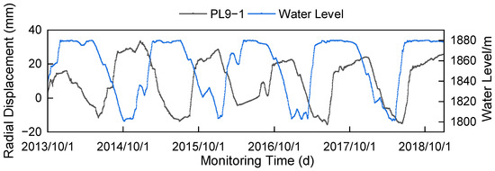
Figure 3.
The radial displacement and the reservoir water level of the NO.9 dam section.
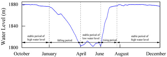
Figure 4.
The water level segmentation interval diagram.
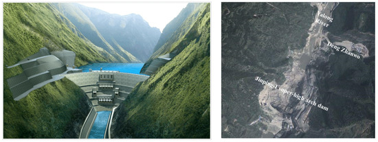
Figure 5.
The simulation of the scenario and the of Jinping-I super-high arch dam.
5. Results and Accuracy of the Proposed Model
5.1. A Better Mathematical Model for the Ageing Displacement of Concrete Dams
To calculate the hydraulic displacement component by the FEM, a three-dimensional FEM model is established using ABAQUS, as shown in Figure 6. The instantaneous elastic modulus of the dam concrete is determined to be 38 GPa, which is an elastic inversion value conducted according to the measured dam displacement during the initial rising period of the upstream reservoir water level, rising from 1800.41 m to 1880 m [44]. The parameters of the foundation rocks are determined by their designed values. The instantaneous elastic modulus E1 and delayed elastic modulus E2 in the Burgers model are determined to be 46.5 GPa and 130.5 GPa. The corresponding viscosity coefficients are 376.2 GPa.d and 20,074.5 GPa.d, respectively. During the simulation period, there are a total of 32 incremental steps in the FEM simulation, with each step resulting in a 5 m change in water level. Figure 7 shows the relationship between the elastic FEM-calculated radial displacement and the upstream reservoir water depth for PL9-1.
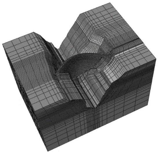
Figure 6.
FEM model of the Jinping-Ⅰ super-high arch dam.
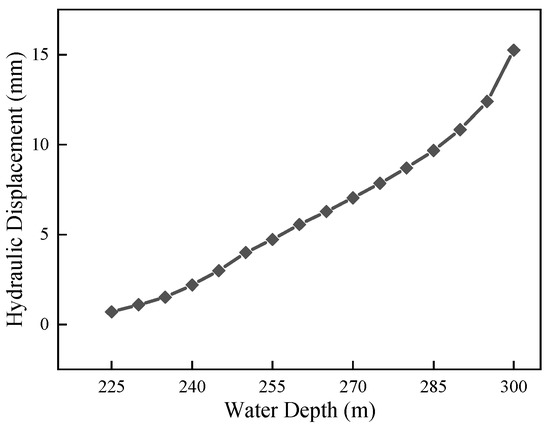
Figure 7.
Relationship between the elastic FEM-calculated radial displacement and the upstream reservoir water depth for PL9-1.
5.2. Calculation of Temperature Displacement by KPCA Method
A large number of thermometers are embedded in the dam body. From the mechanical point of view, the thermometer measurement data of the concrete and rock foundation of the dam should be selected as the temperature factor. The principal component analysis (PCA) method was used in the previous studies [45,46] to analyse and separate the temperature measurement principal component. Its linear technique, on the other hand, has difficulty reducing large amounts of temperature variables to new uncorrelated variables while minimizing the loss of original information. In this paper, the principal components of thermometers are extracted by the KPCA method. As a result, the temperature components can be fitted more precisely. The advantages of using the measured temperatures of the concrete dam have been mentioned and testified by several articles [47,48,49]. In order to approve the KPCA’s high performance on feature extraction and dimensionality reduction of input temperature dataset, the comparison process with PCA is necessarily proposed. The PCA method is based on the assumption that there was a linear hyperplane. The KPCA method is kernel-based, and the mapping performed by the KPCA method highly relies on the choice of the kernel function. Possible choices for the kernel function are the Linear kernel, Gaussian kernel, Polynomial kernel, Sigmoid kernel, and Laplacian kernel [50,51]. Table 1 shows the performance of the KPCA models based on different kernel functions. According to the results, the KPCA method with the Linear kernel, Polynomial kernel, and Sigmoid kernel achieves nearly the same accuracy rate and maximum contribution rate as the first kernel PC. In contrast, the Gaussian kernel and Laplacian kernel approach the low maximum contribution rate of the first kernel PC. As a result, the Polynomial kernel is chosen to replace the linear projection process. Figure 8 depicts the comparison of the two methods in the extraction result. It can conclude that after using the KPCA method with the polynomial kernel, two PCs are extracted. These two PCs can explain approximately 93.65% of the information in the original temperature dataset. They are considered to represent the thermal effect. The PC1, which has the maximum contribution proportion among all the principal components, explains 73.31% of the information in the original temperature dataset. In contrast, after using the PCA method, four PCs are extracted, and the PC1 explains only 46.87% of the information. As a result of using the KPCA method, a small number of principal components from the thermometers can be extracted and used for the temperature component as follows:
where TPCi is the ith extracted temperature principal component; bi is the coefficient of the principal component.

Table 1.
The performance of the KPCA models based on different kernel functions.
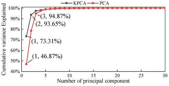
Figure 8.
The comparison of the PCA method and the KPCA method in the extraction result.
5.3. Fitting and Predicting Accuracy of the Proposed Hybrid Model
To test the accuracy of the new hybrid model, the long monitoring data from 1 October 2013 to 31 December 2018 were divided into the training set, and the predicting set [52]. The first 1560 data in the dataset are used as the training set and the last 354 data are used as the predicting set. The coefficients of the Equation (39) are calculated and shown in Table 2. For the Jinping-I super high arch dam, the design and inversion values of the instantaneous elastic modulus of the dam concrete are 38.0 GPa and 38.5 GPa, respectively. As a result, the elastic hydraulic displacement calculated by FEM should be multiplied by the coefficient X of 0.98 (38.0/38.5).
Table 2.
Coefficients of the new hybrid model for PL9-1.
The model results are tested and compared using several estimation criteria, including the mean absolute error MAE, the mean squared error MSE and the determination coefficient R2. The criteria mentioned above can be calculated as follows:
where N is the number of observations; is the predicted displacement value of the model; y is the measured displacement of the concrete dam; and are the mean value of predicted and measured displacement, respectively. The estimation criteria MAE, MSE, and R2 are displayed in Table 3, respectively for the HST model and the proposed hybrid model.
Table 3.
The regression model performance comparison of the proposed model and the HST model.
As can be seen in Table 3, the two models realize the satisfactory performance that the correlation coefficients in the training set and predicting set are both higher than 0.95. The new hybrid model reaches deduced error and higher correlation coefficient than the HST model. It is reasonable to conclude that the model developed in this paper has both a clear physical meaning and a high fitting accuracy. As shown in Figure 9, the more significant error occurs when the measured value changes more violently, that is, when the water level changes more violently. However, the new hybrid model provides better stability in the fitting process compared to the HST model when the water level changes drastically.
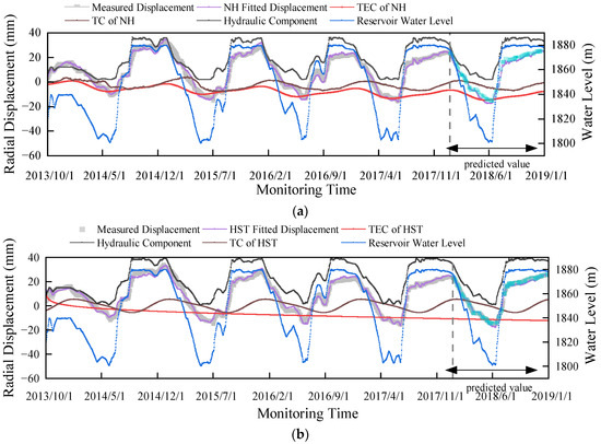
Figure 9.
Fitted process lines for measurement point PL9-1 in the NO.9 dam section: (a): The new hybrid model; (b) The HST hybrid model. Abbreviation: NH: new hybrid model; HST: hydraulic-seasonal-time model; HC: hydraulic component; AC: ageing component; TC: temperature component.
The variation laws and values of the thermal displacement obtained by the new hybrid model and the HST model are displayed in Figure 10. The line temperature component (TC) of HST and the line TC of the new hybrid model (NH) are the ambient temperature of the dam and the internal temperature displacement of the dam, respectively, which both follow a periodic pattern. The internal temperature displacement of the dam has a slight lag relative to the ambient temperature displacement of the dam, in line with the law that the internal temperature of concrete has a phase difference relative to the ambient temperature. This phenomenon has the following possible explanations. The external ambient temperature at any given moment affects the change of its temperature field by means of heat conduction inside the dam concrete, and it takes some time for this heat conduction process to be finally completed. At the same time, the continuous change of external temperature causes the internal heat exchange of the dam body, i.e., when the heat input to the dam body in the current period has not yet been transferred to the deep concrete, the heat input to the dam body in the latter period has already begun to affect the layers of concrete, and so is the next. The slow and continuous heat transfer inside the dam body inevitably leads to the superposition of the influence of the external ambient temperature on the internal temperature field of the dam body at different times, thus causing a lag in the internal temperature field of the dam body relative to the external temperature.
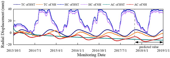
Figure 10.
Radial displacement of hydraulic, thermal and ageing components separated by the HST hybrid model and the new hybrid model. Abbreviation: NH: new hybrid model; HST: hydraulic-seasonal-time model; HC: hydraulic component; AC: ageing component; TC: temperature component.
The ageing displacement separated by the model is a combination of increasing and decreasing curves, containing reversible ageing displacement that varies with the main load of the dam in addition to irreversible trend ageing displacement, and the change in ageing displacement slightly lags behind the change in reservoir level at this stage, in line with the hysteresis effect of viscoelastic deformation. In comparison, the ageing component is expressed as c1θ + c2lnθ in the HST model, which only contains irreversible deformations. The instantaneous and hysteretic elastic hydraulic deformations are owned to the hydraulic component, which will result in larger hydraulic displacement in the HST model, as can be seen in Figure 10. While the hydraulic displacement, which is determined by the evolution of reservoir water level, has an annual evolution law comparable to the reversible ageing displacement in the new hybrid model. Thus, the development trend of the ageing displacement can be better reflected in the new hybrid model. It contains both reversible and irreversible components.
6. Conclusions and Discussion
In this paper, we proposed a new hybrid model for a concrete dam in which the temperature displacement and the ageing displacement of the traditional hybrid model are improved, and the validity and interpretability of the model accuracy of this paper can be confirmed through example validation according to the smaller predicting MSE (0.3404) and larger R2 (0.9902), whereas in the traditional HST hybrid model they are 2.2055 and 0.9898, respectively. The following conclusions are drawn:
- (1)
- The principal component factors are extracted using kernel principal component analysis in conjunction with measured thermometer information in the concrete dam body, which can better reflect the influence of temperature variations inside the concrete dam body on its displacement compared with the traditional HST hybrid model.
- (2)
- The Burgers model was used to determine the instantaneous elasticity modulus and viscoelastic modulus of the dam; thus the hysteretic hydraulic elastic displacement in the original hybrid model can be subsumed into the ageing displacement component, while the period factor was added to the ageing displacement to fit this component. Thus, a better mathematical model for the ageing displacement of concrete dams was established. It can fully reflect the recoverable creep component of the concrete and rock and accurately separate the ageing component from the total displacement.
However, some problems also should be pointed out. Firstly, the effectiveness of the proposed model is only validated in the experimental conditions. It needs to be applied in the actual engineering programs to verify the practicability. Moreover, the time range of the ageing deformation selected in this paper is only from 2013 to 2018, but the ageing deformation of the dam, especially in the stability period, will last for a long time. The change of water level component, temperature component, and ageing component for a longer time need to be discussed.
Author Contributions
Conceptualization, M.Y. and C.G.; methodology, X.C.; software, H.G.; validation, M.Y., X.C., H.G. and C.G.; formal analysis, M.Y.; investigation, X.C.; resources, H.G.; data curation, C.G.; writing—original draft preparation, M.Y. and X.C.; writing—review and editing, M.Y., X.C., H.G. and C.G. All authors have read and agreed to the published version of the manuscript.
Funding
This work was supported by the China Postdoctoral Science Foundation (Grant No. 2022M721668, 2021M701044); Central Public-Interest Scientific Institution Basal Research Fund, NHRI (Y423006, Y423004); the National Natural Science Foundation of China (51739008, U2243223, 51739003, 51779086 and 52079046); Science and technology projects managed by the headquarter of State Grid Corporation (5108-202218280A-2-417-XG); the Fundamental Research Funds for the Central Universities of Hohai (Grant No. B230201011); the Open Fund of Research Center on Levee Safety Disaster Prevention of Ministry of Water Resources under Grant (LSDP202204); Water Conservancy Science and Technology Project of Jiangsu (Grant No. 2022024); the National Natural Science Foundation for Young Scientists of China (Grant No. 51909173); Open fund of the National Dam Safety Research Center (Grant No. CX2020B02); The Fundamental Research Funds for the Central Universities (B210202017); the Jiangsu young science and technological talents support project (TJ-2022-076); the Open Fund of National Dam Safety Research Center (CX2020B02) and the Anhui Natural Sci-ence Foundation grant number (Grant No. 2208085US17).
Institutional Review Board Statement
Not applicable.
Informed Consent Statement
Not applicable.
Data Availability Statement
The data presented in this study are available on request from the corresponding author. The data are not publicly available due to project confidentiality.
Conflicts of Interest
The authors declare that there are no conflict of interest.
References
- Liu, Y.Z.; Li, J.T.; Chen, W.F.; Zhang, G.X.; Tan, Y.S. Optimization study on super-high arch dam temperature control standard and measure. In Proceedings of the 4th International Workshop on Renewable Energy and Development (IWRED), Sanya, China, 24–26 April 2020; Electr Network. Volume 510. [Google Scholar]
- Zhang, C.; Ali, A.; Sun, L. Investigation on low-cost friction-based isolation systems for masonry building structures: Experimental and numerical studies. Eng. Struct. 2021, 243, 112645. [Google Scholar] [CrossRef]
- Wang, S.; Xu, C.; Gu, C.; Su, H.; Wu, B. Hydraulic-seasonal-time-based state space model for displacement monitoring of high concrete dams. Trans. Inst. Meas. Control. 2021, 43, 3347–3359. [Google Scholar] [CrossRef]
- Huang, H.; Li, M.; Yuan, Y.; Bai, H. Experimental Research on the Seismic Performance of Precast Concrete Frame with Replaceable Artificial Controllable Plastic Hinges. J. Struct. Eng. 2023, 149, 04022222. [Google Scholar] [CrossRef]
- Zhang, Z.; Liang, G.; Niu, Q.; Wang, F.; Chen, J.; Zhao, B.; Ke, L. A Wiener degradation process with drift-based approach of determining target reliability index of concrete structures. Qual. Reliab. Eng. Int. 2022, 38, 3710–3725. [Google Scholar] [CrossRef]
- Huang, H.; Li, M.; Yuan, Y.; Bai, H. Theoretical analysis on the lateral drift of precast concrete frame with replaceable artificial controllable plastic hinges. J. Build. Eng. 2022, 62, 105386. [Google Scholar] [CrossRef]
- Gu, M.; Cai, X.; Fu, Q.; Li, H.; Wang, X.; Mao, B. Numerical Analysis of Passive Piles under Surcharge Load in Extensively Deep Soft Soil. Buildings 2022, 12, 1988. [Google Scholar] [CrossRef]
- Deng, E.-F.; Zhang, Z.; Zhang, C.-X.; Tang, Y.; Wang, W.; Du, Z.-J.; Gao, J.-P. Experimental study on flexural behavior of UHPC wet joint in prefabricated multi-girder bridge. Eng. Struct. 2023, 275, 115314. [Google Scholar] [CrossRef]
- Cheng, Y.; Fu, L.-Y. Nonlinear seismic inversion by physics-informed Caianiello convolutional neural networks for overpressure prediction of source rocks in the offshore Xihu depression, East China. J. Pet. Sci. Eng. 2022, 215, 110654. [Google Scholar] [CrossRef]
- Chen, J.H.; Gu, C.S. Study on Semi-parametric Statistical Model of Safety Supervision of Concrete Dam. Disaster Adv. 2013, 6, 16–24. [Google Scholar]
- Shang, C. Statistical analysis of deformation monitoring data of a RCC gravity dam. J. Water Resour. Water Eng. 2017, 28, 205–211. [Google Scholar]
- Hu, J.; Wu, S. Statistical modeling for deformation analysis of concrete arch dams with influential horizontal cracks. Struct. Health Monit. 2019, 18, 546–562. [Google Scholar] [CrossRef]
- Kang, F.; Liu, X.; Li, J. Temperature effect modeling in structural health monitoring of concrete dams using kernel extreme learning machines. Struct. Health Monit. 2020, 19, 987–1002. [Google Scholar] [CrossRef]
- Chen, Y.; Xiao, G.; Hu, M.; Huang, J. Dam deformation prediction based on extreme learning machine and elastic network. Sci. Surv. Mapp. 2020, 45, 20. [Google Scholar]
- Su, H.; Wen, Z.; Wu, Z. An Early-warning Model of Dam Safety Based on SVM Theory. J. Basic Sci. Eng. 2009, 17, 40–48. [Google Scholar]
- Salazar, F.; Toledo, M.; Oñate, E.; Suárez, B. Interpretation of dam deformation and leakage with boosted regression trees. Eng. Struct. 2016, 119, 230–251. [Google Scholar] [CrossRef]
- Campos, A.; López, C.M.; Blanco, A.; Aguado, A. Structural Diagnosis of a Concrete Dam with Cracking and High Nonrecoverable Displacements. J. Perform. Constr. Facil. 2016, 30, 04016021. [Google Scholar] [CrossRef]
- Lamea, M.; Mirzabozorg, H. Simulating Structural Responses of a Generic AAR-Affected Arch Dam Considering Seismic Loading. Sci. Iran 2018, 25, 2926–2937. [Google Scholar] [CrossRef]
- Wang, S.; Xu, C.; Gu, H.; Zhu, P.; Liu, H.; Xu, B. An Approach for Quantifying the Influence of Seepage Dissolution on Seismic Performance of Concrete Dams. Comput. Model. Eng. Sci. 2022, 131, 97–117. [Google Scholar] [CrossRef]
- Li, F.; Wang, Z.; Liu, G.; Fu, C.; Wang, J. Hydrostatic seasonal state model for monitoring data analysis of concrete dams. Struct. Infrastruct. Eng. 2015, 11, 1616–1631. [Google Scholar] [CrossRef]
- Wang, S.; Xu, Y.; Gu, C.; Bao, T.; Xia, Q.; Hu, K. Hysteretic effect considered monitoring model for interpreting abnormal deformation behavior of arch dams: A case study. Struct. Control. Health Monit. 2019, 26, e2417. [Google Scholar] [CrossRef]
- Gu, C.S.; Wu, Z.R. Safety Monitoring of Dams and Dam Foundations: Theories & Methods and Their Application. 2006. Available online: https://www.scopus.com/inward/record.uri?eid=2-s2.0-85119970332&partnerID=40&md5=b759974ac898b3b32a5e01140f7cd34f (accessed on 14 December 2022).
- Hu, J.; Ma, F. Zoned deformation prediction model for super high arch dams using hierarchical clustering and panel data. Eng. Comput. 2020, 37, 2999–3021. [Google Scholar] [CrossRef]
- Tatin, M.; Briffaut, M.; Dufour, F.; Simon, A.; Fabre, J.-P. Thermal displacements of concrete dams: Accounting for water temperature in statistical models. Eng. Struct. 2015, 91, 26–39. [Google Scholar] [CrossRef]
- Mata, J.; de Castro, A.T.; da Costa, J.S. Time–frequency analysis for concrete dam safety control: Correlation between the daily variation of structural response and air temperature. Eng. Struct. 2013, 48, 658–665. [Google Scholar] [CrossRef]
- Kang, F.; Li, J.; Zhao, S.; Wang, Y. Structural health monitoring of concrete dams using long-term air temperature for thermal effect simulation. Eng. Struct. 2019, 180, 642–653. [Google Scholar] [CrossRef]
- Chen, S.; Gu, C.; Lin, C.; Zhao, E.; Song, J. Safety Monitoring Model of a Super-High Concrete Dam by Using RBF Neural Network Coupled with Kernel Principal Component Analysis. Math. Probl. Eng. 2018, 2018, 1712653. [Google Scholar] [CrossRef]
- Zhang, J.; Richards, C.M. Parameter identification of analytical and experimental rubber isolators represented by Maxwell models. Mech. Syst. Signal Process. 2007, 21, 2814–2832. [Google Scholar] [CrossRef]
- Pelosi, G. The finite-element method, part 1: R. L. Courant. IEEE Antennas Propag. Mag. 2007, 49, 180–182. [Google Scholar] [CrossRef]
- Ren, S.; Zhao, G.; Zhang, S. Elastic–Viscoelastic Composite Structures Analysis with an Improved Burgers Model. J. Vib. Acoust. 2018, 140, 031006. [Google Scholar] [CrossRef]
- Xiong, L.; Yang, L.; Zhang, Y. Non-stationary Burgers model for rock. J. Cent. South Univ. 2010, 41, 679–684. [Google Scholar]
- Zhang, S.; Sheng, D.; An, W.; Liu, B.; Qi, R.; Cheng, J. Nonlinear Visco-Elastic-Plastic Analysis of Rubber Asphalt Composites Based on Improved Burgers Model. Chin. Q. Mech. 2021, 42, 528–537. [Google Scholar]
- Huang, Y.; Wan, Z. Study on Viscoelastic Deformation Monitoring Index of an RCC Gravity Dam in an Alpine Region Using Orthogonal Test Design. Math. Probl. Eng. 2018, 2018, 8743505. [Google Scholar] [CrossRef]
- Hu, Y.; Gu, C.; Meng, Z.; Shao, C. Improve the Model Stability of Dam’s Displacement Prediction Using a Numerical-Statistical Combined Model. IEEE Access 2020, 8, 147482–147493. [Google Scholar] [CrossRef]
- Ranaivomanana, N.; Multon, S.; Turatsinze, A. Basic creep of concrete under compression, tension and bending. Constr. Build. Mater. 2013, 38, 173–180. [Google Scholar] [CrossRef]
- Mei, S.; Wang, Y.; Zou, R.; Long, Y.; Zhang, J. Creep of concrete-filled steel tube considering creep-recovery of the concrete core. Adv. Struct. Eng. 2020, 23, 997–1009. [Google Scholar] [CrossRef]
- Ju, Y.-W.; Li, K.-F.; Han, J.-G. Experimental and theoretical research on tensile creep of early-age concrete. Eng. Mech. 2009, 26, 43–49. [Google Scholar]
- Gu, C.S.; Zhao, E.F. Theory and Method of dam Safety Monitoring; Hohai University Press: Nanjing, China, 2019. [Google Scholar]
- Yang, C.; Chen, M.; Zhang, M.; Li, Q.; Fang, W.; Wen, Q. Research on the creep of concrete filled steel tubular columns based on the generalized kelvin chain. Eng. Mech. 2022, 39, 200–207. [Google Scholar]
- Yakubovskiy, Y.E.; Kolosov, V.I.; Donkova, I.A.; Kruglov, S.O. Creep mathematical model on the example of early age concrete. IOP Conf. Ser. Mater. Sci. Eng. 2020, 972, 012054. [Google Scholar] [CrossRef]
- Sun, K.; Wu, Z.D.; Wu, Y.Y.; Wu, Y.Z. Research on fault diagnosis of altimeter based on KPCA-BN. J. Ordnance Equip. Eng. 2020, 41, 95–99. [Google Scholar]
- Li, X.; Zhang, L.; Khan, F.; Han, Z. A data-driven corrosion prediction model to support digitization of subsea operations. Process. Saf. Environ. Prot. 2021, 153, 413–421. [Google Scholar] [CrossRef]
- Su, H.; Wen, Z.; Ren, J. A kernel principal component analysis-based approach for determining the spatial warning domain of dam safety. Soft Comput. 2020, 24, 14921–14931. [Google Scholar] [CrossRef]
- Wang, S.; Xu, C.; Su, H. Back analysis of viscoelastic working behavior for Jinping-I Arch Dam. Adv. Sci. Technol. Water Resour. 2020, 40, 62–69. [Google Scholar]
- Li, Y.; Bao, T.; Shu, X.; Chen, Z.; Gao, Z.; Zhang, K. A Hybrid Model Integrating Principal Component Analysis, Fuzzy C-Means, and Gaussian Process Regression for Dam Deformation Prediction. Arab. J. Sci. Eng. 2021, 46, 4293–4306. [Google Scholar] [CrossRef]
- Ren, L.; Song, C.; Wu, W.; Guo, M.; Zhou, X. Reservoir effects on the variations of the water temperature in the upper Yellow River, China, using principal component analysis. J. Environ. Manag. 2020, 262, 110339. [Google Scholar] [CrossRef]
- Su, H.; Li, J.; Hu, J.; Wen, Z. Analysis and Back-Analysis for Temperature Field of Concrete Arch Dam During Construction Period Based on Temperature Data Measured by DTS. IEEE Sens. J. 2013, 13, 1403–1412. [Google Scholar] [CrossRef]
- Yang, M.; Su, H. A study for optical fiber multi-direction strain monitoring technology. Optik 2017, 144, 324–333. [Google Scholar] [CrossRef]
- Xu, B.; Liu, B.; Zheng, D.; Chen, L.; Wu, C. Analysis method of thermal dam deformation. Sci. China Technol. Sci. 2012, 55, 1765–1772. [Google Scholar] [CrossRef]
- Yang, M.; Su, H.; Wen, Z. An approach of evaluation and mechanism study on the high and steep rock slope in water conservancy project. Comput. Concr. 2017, 19, 527–535. [Google Scholar] [CrossRef]
- Halim, H.; Isa, S.M.; Mulyono, S. Comparative analysis of PCA and KPCA on paddy growth stages classification. In Proceedings of the IEEE Region 10 Symposium (TENSYMP), Sanur, Indonesia, 9–11 May 2016; pp. 167–172. [Google Scholar]
- Shao, C.; Zheng, S.; Gu, C.; Hu, Y.; Qin, X. A novel outlier detection method for monitoring data in dam engineering. Expert Syst. Appl. 2022, 193, 116476. [Google Scholar] [CrossRef]
Disclaimer/Publisher’s Note: The statements, opinions and data contained in all publications are solely those of the individual author(s) and contributor(s) and not of MDPI and/or the editor(s). MDPI and/or the editor(s) disclaim responsibility for any injury to people or property resulting from any ideas, methods, instructions or products referred to in the content. |
© 2023 by the authors. Licensee MDPI, Basel, Switzerland. This article is an open access article distributed under the terms and conditions of the Creative Commons Attribution (CC BY) license (https://creativecommons.org/licenses/by/4.0/).