Identifying Key Indicators for Monitoring Water Environmental Services Payment Programs—A Case Study in Brazil

Abstract

The recognition of the natural environment as an element that provides ecosystem services to society has led to an increased interest in the study of these services and the implementation of payment for environmental services (PES) initiatives. Although in recent years it has gained strength as an environmental conservation and restoration strategy, the PES instrument lacks something in the monitoring of its actions that inhibits its concrete efficiency, such as indicators that represent the study area. Based on the results of water, soil, and vegetation quality reported in a case study on a rural property participating in a PES-Water scheme in Brazil, the present study aimed to establish minimum water quality indicators relevant to the monitoring of PES-Water programs and propose a flowchart for monitoring actions and environmental aspects to support future projects of the same nature. Based on the results, the monitoring of these areas must involve the continuous checking of soil indicators, water and vegetation. In addition, details of the microclimate and socioeconomic conditions must be recorded. The results should also be systematized, disseminated, and made available in a monitoring system to serve the various actors involved, thereby facilitating the understanding of the PES instrument and the remuneration for the environmental services provided.

1. Introduction

Ecosystem services make significant contributions to human welfare; some are essential and cannot be replaced and almost all are becoming increasingly scarce [1]. There are real costs to providing ecosystem services, and we must develop suitable mechanisms for paying for them. Payment for ecosystem services is becoming increasingly popular as a way to manage ecosystems using economic incentives [1,2]. Such monitoring of ecosystem services is mandated by a suite of recent multilateral political agreements and (inter)national assessments that have adopted the ecosystem service framework; these include the Intergovernmental Science Policy Platform on Biodiversity & Ecosystem Services (IPBES) [3], the Aichi Biodiversity Targets [4], the European Union (EU) Biodiversity Strategy [5], and the recent US memorandum directing federal agencies to factor ecosystem services into planning and decision making [6]. An example of an initiative in the face of these agreements is the role of The Group on Earth Observations Biodiversity Observation Network—GEOBON, which focuses on monitoring biodiversity and ecosystem services at the global level [7].

In addition to complying with regulations and agreements, the supervision of activities proposed in a PES program through periodic assessments is used to understand the range of the provision of ecosystem services under these programs [8]. The monitoring data must be linked to the results of the initial projects to highlight the quality and frequency of the available information [9].

The effectiveness of the monitoring ensures reliability for the people involved, and when it is disclosed along with details of the methodologies used it serves as an instrument for validating the method, in addition to providing support for future projects [10,11]. On the other hand, its absence limits the environmental performance of PES programs and entails difficulty in understanding the quality and quantity of services provided [12,13,14].

For continuous monitoring that faithfully represents reality, it is necessary to establish (i) parameters consistent with the study ecosystem, which can be monitored in the medium and long term, that are low cost, effective, and easy to apply, and capable of diagnosing the status of the environment and measuring the desired changes in the environmental, social and economic aspects; (ii) a minimum frequency of monitoring consistent with the adopted indicators, which requires knowledge and technical support [15,16].

These parameters, for now termed “indicators”, serve to warn about a phenomenon, problem, challenge, or established goal [17]. They can be used for a wide range of purposes, such as measuring food production, water supply, water regulation and habitat maintenance. In PES programs, the indicators act as a key element to provide information on the evolution of the program with respect to the established goals. Furthermore, when crossed with information from regions not considered in the application of the program, they make it possible to highlight the changes in the ecosystem arising from the implementation of PES for environmental quality and human well-being [18].

Although there has been a growing interest in monitoring ecosystem services, whether in terms of spatialization in the light of natural supply or the scope of PES schemes, several governments have not been successful in measuring and monitoring these services [19], and even lack indicators and monitoring approaches that can be applied on a global scale and serve to support decision making [20]. Monitoring these services has created one of the main bottlenecks for the proper efficiency of the said instrument, mainly due to the failure to obtain and/or disseminate information or its absence and cost of implementation, thus compromising the achievement of the established objectives [15,21,22].

Therefore, the objectives of this study are to (i) evaluate the spatial–temporal variability of water quality parameters relevant to PES program initiatives; (ii) analyze the spatial variation of the properties of the soil and vegetation cover and its correlation with the physical–chemical characteristics of the water; and (iii) propose a PES-Water monitoring scheme based on the previous results.

2. Materials and Methods

The present study was developed from the results obtained in a case study carried out on a rural property participating in a payment for environmental services (PES) program with a water focus in the municipality of Campinas, in the state of São Paulo, Brazil. The region is influenced by the tropical Atlantic and continental and polar Atlantic air masses and is classified as Cfb (temperate with mild summer), Cfa (subtropical with hot summer), and Cwa (subtropical with dry winter and hot summer) under the Köppen climate classification system. The rainy season starts in the spring, especially in October, and lasts until mid-April with a peak in the summer and a drought from May to September, so that the precipitation values are between 1200 and 1800 mm annually [23,24].

Data from the Integrated Center for Agrometeorological Information (Centro Integrado de Informações Agrometeorológicas) [25] indicate that in the period of study between April 2019 and September 2020, the average temperature in the municipality was 22.3 °C, with October being the hottest month, with a monthly average of 25.4 °C, and with July being the coldest month, with a monthly average of 19.1 °C. As for precipitation in the same period, the municipality had an average of 81.9 mm, with a higher monthly average in February 2020 of 214.9 mm and a lower average for April 2020.

Details of the property used for the study, the location of which is given in Figure 1, were gathered in the PES program in February 2018. It has an area of 102.9 ha, of which 14.4 ha is a permanent preservation area (APP), 16.8 ha is the remaining vegetation, and 58.3 ha is pasture, with livestock rearing as the main activity.

The Customized Property Program under the PES defined goals and actions that are subdivided into four blocks: (i) forest code, which covers the legal obligations for forest restoration and protection of native vegetation; (ii) rural sanitation, which deals with domestic effluent management and rainwater drainage actions; (iii) soil conservation, which relates to the implementation and maintenance of soil conservation practices; and (iv) granting the use of water resources.

Seven bimonthly follow-up points were defined, the brief description of which is given in

Table 1. Environmental characterization of sampling points.

Point	Description	Spatial Representation
1	Downstream property External point Quality of water leaving the property Unpaved road
2	Test Pit Forest remnant External course Access way PES planting
3	Sewer amount Before the treatment system and external course Higher water flow
4	Erosive process Conservation practices Low water density Burlap
5	Consumption—nascent Spring displacement Livestock amount Fencing
6	Livestock interference Cattle trampling PES surrounding Downstream planting
7	Property amount Prior to improvements Siltation Drainage work

. They determine the degree of water quality, given the spatial distribution on the property, and ascertain whether the results obtained are associated with the measures adopted or whether they reflect the seasonality of precipitation.

2.1. Water Quality

The water sampling took place in April 2019, July 2019, September 2019, November 2019, and January 2020, with four samples being taken at each point for statistical analysis. The first stage of water quality analysis consisted of measuring the following parameters: dissolved oxygen—DO (oximeter), biochemical oxygen demand—BOD (oximeter and incubation), pH (potentiometer), temperature (oximeter), turbidity (turbidimeter), electrical conductivity (conductivity meter), total dissolved solids—TDS (gravimetry), total phosphorus (ascorbic acid method), total nitrogen (Kjeldahl digestion and distillation), and total coliforms (multiple tubes).

The water data were subjected to a descriptive statistical analysis (mean, standard deviation, and variation coefficient) to understand the variability of the limnological indicators used, and later a principal component analysis (PCA) was applied to the data set to assess the contribution of each indicator to the spatial–temporal variability of quality. This approach allows us to assess which variable has the greatest weight in statistical analysis and which are the most important variables from a statistical point of view [26].

2.2. Soil Quality

To assist the understanding of spatial changes in water quality indicators, especially regarding the physical–chemical characteristics of the soil and if they influence the analyzed water parameters, single surface soil samples were collected with the aid of an auger. The parameters analyzed are shown in

Table 2. Soil quality parameters and measurement methods.

Parameters		Determination
Micronutrients (mg/dm3)	Copper (Cu)	DTPA
	Iron (Fe)	DTPA
	Manganese (Mn)	DTPA
	Zinc (Zn)	DTPA
	Boron (B)	Hot Water
Macronutrients (mg/dm3 for P) (mmolc/dm3 for Ca and Mg)	Calcium (Ca)	Resin
	Magnesium (Mg)	Resin
	Phosphorus (P)	Resin
Cation exchange capacity—CEC (mmolc/dm3)		Calculation according to IAC methodology [27]
Base saturation	V%	Calculation according to IAC methodology [27]
Acidity	Active − pH	CaCl2
	Total − H + AL (mmolc/dm3)	Calculation according to IAC methodology [27])
Particle size distribution (g/Kg)	Clay	HMFS + NaOH
	Silt	HMFS + NaOH
	Total sand	HMFS + NaOH
Organic matter (g/dm3)		Oxidation

. It is noteworthy that there were no repetitions per sampling point, and there was a lack of measurement in different sampling months.

2.3. Vegetation Cover Quality

Like that adopted for soil quality indicators, a vegetation quality indicator was used to register any associations between it and water quality parameters. The parameter used to analyze the vegetation was the leaf area index (LAI). This study assessed it by means of hemispheric photographs, which can map the size, magnitude, and distribution of the canopy openings with the location where the photograph was taken [28], so that the higher the LAI value, the better the vegetation density [29].

The photographs were taken with a north orientation at the sampling points, at a height of 1.3 m in a single sample using a Cyber-shot^® Digital Camera Sony DSC—F828 camera with a Fisheye Opteka^® 0.22X AF lens attached, and analyzed in HemiView ©, version 2.1; Software for convenient image analysis of hemispherical photography; Delta-T Devices, University of Kansas Centre for Research, David A. Vieglais and He-lios Environmental Modelling Institute: Burwell, Cambridge, UK, 1999, classifying light (white pixels) and plant biomass (black pixels).

2.4. PES-Water Monitoring Plan

Considering the need and the difficulty in monitoring PES-Water programs, mainly due to the availability of technical personnel, financial resources, equipment, and the edaphoclimatic characteristics of the places of interest, and with the data collected by this study on the property, it is proposed to carry out a monitoring scheme with a view to gaining the benefits generated by applying the program in rural properties.

To support the monitoring program proposal, a correlation analysis was performed on the indicators of the soil–water–vegetation aspects, considered through the application of the Pearson correlation coefficient. This is a measure of the linear association between variables [30] varying between −1 and 1, so that the positive or negative sign indicates the direction of the association between the considered variables. In situations of null correlation, with an r value close to zero, there is usually no association between the variables [31]. Because these extremes are hardly reached, the authors of [30] suggest a classification with intermediate ranges of interpretation to be considered: an r coefficient between 0.10 and 0.30 as the weak degree of correlation, that from 0.40 to 0.60 as a moderate correlation and that from 0.70 to 1 as strong correlation.

3. Results

3.1. Spatial–Temporal Variation of Water Quality Indicators

Table 3. Water quality per sampling point in the study property, Campinas, Brazil.

	Dissolved Oxygen (mg/L)			Biochemical Oxygen Demand (mg/L)			pH			Turbidity (NTU)
Point	Average	SD	CV (%)	Average	SD	CV (%)	Average	SD	CV (%)	Average	SD	CV (%)
1	6.61 b	1.38	20.91	3.39 d	1.27	37.50	7.35 d	0.26	3.49	16.29 c	8.75	53.76
2	6.53 b	1.85	28.36	3.18 bc	1.59	49.92	7.26 c	0.41	5.70	19.43 d	22.85	117.57
3	6.21 a	1.76	28.42	3.08 b	1.52	49.17	7.20 bc	0.33	4.54	8.73 b	5.06	57.93
4	5.65 d	1.69	29.88	2.91 a	1.44	49.32	7.04 a	0.24	3.35	39.44 f	28.41	72.02
5	5.18 c	1.36	26.21	2.55 e	1.09	42.60	7.09 a	0.26	3.66	23.29 e	8.01	34.39
6	6.22 a	1.92	30.83	3.30 cd	1.56	47.39	7.18 b	0.22	3.02	48.92 g	17.24	35.24
7	6.18 a	1.69	27.41	2.78 a	1.30	46.65	7.07 a	0.24	3.44	7.09 a	5.54	78.10
	Temperature (°C)			Electrical Conductivity (µs/cm)			Total Dissolved Solids (mg/L)			Total Phosphorus (mg/L)
Point	Average	SD	CV (%)	Average	SD	CV (%)	Average	SD	CV (%)	Average	SD	CV (%)
1	20.68 c	0.69	3.31	101.81 a	7.48	7.35	141.30 c	43.34	30.67	0.03 a	0.02	63.95
2	19.18 a	0.51	2.67	101.56 a	26.48	26.07	160.80 d	56.08	34.88	0.06 b	0.07	114.05
3	21.06 d	0.44	2.11	108.55 f	8.68	8.00	210.00 b	52.22	24.87	0.06 b	0.05	96.62
4	20.03 b	0.36	1.80	98.50 e	7.35	7.46	226.40 a	76.78	33.91	0.09 e	0.12	131.65
5	18.95 a	0.23	1.22	95.02 c	5.75	6.06	235.90 a	54.52	23.11	0.05 c	0.03	57.37
6	21.73 e	0.28	1.28	96.29 d	7.46	7.75	269.50 e	63.48	23.55	0.08 d	0.04	48.51
7	20.27 b	0.48	2.38	75.17 b	18.74	24.93	227.80 ab	73.76	32.38	0.03 a	0.02	50.91
	Total Nitrogen (mg/L)			Total Coliforms (NMP/100 mL)
Point	Average	SD	CV (%)	Average	SD	CV (%)
1	25.67 a	18.30	71.30	1600.00 a	-	-
2	13.52 a	19.58	144.78	1600.00 a	-	-
3	25.12 a	33.70	134.17	1600.00 a	-	-
4	22.33 a	16.15	72.30	1600.00 a	-	-
5	13.10 a	15.48	118.25	1600.00 a	-	-
6	25.17 a	16.41	65.20	1600.00 a	-	-
7	33.12 a	43.27	130.64	1600.00 a	-	-

SD—standard deviation; CV—coefficient of variation. Averages followed by the same lower case do not differ chronically from each other by the Tukey Test at 5% probability to the sampling site. 1. Downstream property; 2. native forest; 3. sewer amount; 4. erosive process; 5. consumption—nascent; 6. livestock interference; 7. property amount.

shows the average sampling values per sampling point for water quality parameters together with their variation coefficients and standard deviation (SD).

The water quality indicators raised for the bimonthly monitoring points showed medium to high dispersion; that is, there was a low homogeneity of data for the parameters of DO, BOD, turbidity, total dissolved solids, total phosphorus, and nitrogen, while the pH parameters, temperature, and electrical conductivity showed low dispersion.

To select the most relevant components for the present study,

Table 4. Explained variance of sample data.

	April 2019			July 2019			September 2019
Comp.	Initial Eigenvalues			Initial Eigenvalues			Initial Eigenvalues
	Total	% Var.	% Accum.	Total	% Var.	% Accum.	Total	% Var.	% Accum.
F1	2.82	31.33	31.33	3.27	36.39	36.388	4.07	45.17	45.17
F2	2.23	24.78	56.10	2.81	31.18	67.564	2.15	23.89	69.06
F3	1.29	14.38	70.48	1.56	17.38	84.945	1.42	15.73	84.79
F4	1.07	11.90	82.38	0.70	7.81	92.761	0.90	10.05	94.84
F5	0.74	8.25	90.64	0.29	3.25	96.016	0.28	3.09	97.93
F6	0.47	5.27	95.91	0.22	2.49	98.506	0.12	1.35	99.28
F7	0.32	3.60	99.51	0.08	0.85	99.360	0.05	0.52	99.81
F8	0.03	0.32	99.83	0.04	0.44	99.804	0.01	0.15	99.95
F9	0.01	0.17	100.00	0.02	0.20	100.00	0.004	0.05	100.00
	November2019			January 2020
Comp.	Initial eigenvalues			Initial eigenvalues
	Total	% Var.	% Accum.	Total	% Var.	% Accum.
F1	3.17	35.28	35.28	3.77	41.90	41.90
F2	2.75	30.56	65.84	2.08	23.08	64.98
F3	1.48	16.45	82.29	1.17	12.99	77.97
F4	1.19	13.20	95.49	0.952	10.58	88.55
F5	0.33	3.70	99.19	0.52	5.78	94.33
F6	0.03	0.32	99.51	0.45	4.95	99.29
F7	0.02	0.22	99.74	0.04	0.40	99.69
F8	0.02	0.17	99.91	0.02	0.26	99.95
F9	0.01	0.09	100.00	0.005	0.05	100.00

Comp—component, Var = variance; Accum. = accumulated; F1 to F9—components.

shows the percentage of total variance explained by each component associated with its respective eigenvalue.

According to Kaiser’s criteria [32], the main components with eigenvalues greater than one were initially considered. Therefore, the nine original components (F1 to F9) could be reduced by three or four new components, depending on the sample.

Table 5. Factor load matrix of water quality variables in selected main components.

Parameters	April 2019				July 2019			September 2019
	F1	F2	F3	F4	F1	F2	F3	F1	F2	F3
DO	−0.682	0.698	0.125	0.048	−0.871	0.430	0.125	0.704	−0.100	−0.672
BOD	−0.530	0.774	0.186	−0.258	−0.551	0.734	0.186	0.909	0.049	−0.308
pH	−0.439	−0.259	−0.261	0.210	−0.521	0.726	−0.261	0.860	−0.247	0.360
Turb	0.728	0.586	0.260	−0.303	0.734	0.498	0.260	−0.099	0.753	0.557
Temp	0.123	0.634	−0.236	0.273	0.219	0.879	−0.236	0.692	0.586	−0.283
EC	0.205	0.271	0.799	−0.214	0.204	0.428	0.799	0.539	−0.696	0.367
TDS	0.765	−0.182	−0.257	−0.049	0.868	0.163	−0.257	0.863	−0.060	0.413
TP	0.801	0.466	0.512	0.593	0.566	0.190	0.512	0.566	0.009	0.195
TN	−0.254	0.086	−0.597	−0.159	0.490	0.537	−0.597	0.400	0.824	0.075
Parameters	November 2019				January 2020
	F1	F2	F3	F4	F1	F2	F3
DO	−0.104	0.828	0.199	−0.238	−0.746	0.062	0.466
BOD	−0.762	0.043	0.248	0.589	−0.833	0.295	0.341
pH	0.538	0.608	−0.130	0.560	0.833	−0.281	0.268
Turb	0.102	−0.294	0.870	0.364	−0.149	−0.706	−0.336
Temp	−0.039	0.645	0.597	−0.417	0.034	0.879	−0.053
EC	0.664	0.609	−0.346	0.239	−0.797	0.238	−0.241
TDS	0.868	−0.343	0.186	−0.288	0.867	0.375	−0.154
TP	0.916	0.164	0.308	0.136	0.320	0.659	−0.280
TN	−0.499	0.822	−0.002	−0.072	0.561	0.078	0.699

F1 to F4—components; DO—dissolved oxygen; BOD—biochemical oxygen demand; Turb—turbidity; Temp—temperature; EC—electrical conductivity; TDS—total dissolved solids; TP—total phosphorus; and TN—total nitrogen (all variables, except total coliforms, which did not differ between themselves). The factor above 0.75 indicates a strong association between.

presents the factorial load matrix of the water quality variables in the selected components. The highest values of the factor weights point to the most significant variables in each factor.

Similar to what was found by [33,34,35], in the analysis of water quality indicators it is suggested that factors with a factor load greater than 0.75 tend to be indicative of a strong association. This justifies the adoption, in Figure 2, of two components in association matrices between components and indicators. There is an average accumulated variance of 64.71% of the data variability (April 2019 = 56.11%, July 2019 = 67.56%, September 2019 = 69.06%, November 2019 = 65.84% and January 2020 = 64.98%).

It can be seen from Figure 2 that in all samplings, Component 1 (F1) is associated in the first or second degree with the parameter total dissolved solids—TDS—that is, the TDS parameter appears between the two prominent indicators of the first component in all of the sampling points, associating with each other the TP indicator for the sampling of April 2019 and November 2019, the OD for July 2019 and the BOD for September 2019 and January 2020.

Component 2 (F2), on the other hand, exhibits variable behavior between the indicators, depending on the sample. For the April 2019 and July 2019 samples, whose precipitation before sampling was at the lowest rates relative to that of the other samples, this component is related to the BOD parameter, corroborating the increase in the BOD value in the context of low rates due to the accumulation of pollutants in the water body. In the September and November samples, the TN indicator is associated with this component. Meanwhile, in the January samples, there is a strong association of this component with the parameters of temperature and turbidity, demonstrating the potential for disintegration, displacement, and carrying soil particles to bodies of water when precipitation occurs.

3.2. Spatial Variation of Soil Properties and Vegetation Cover

Table 6. Physical–chemical characteristics of soils and leaf area index (LAI) at sample points.

	--------Micronutrients (mg/dm3)-------					-------Macronutrients-------			pH	H + Al	V%	CEC (mmolc/dm3)
Point	Cu	Fe	Mn	Zn	B	P	Ca	Mg
1	2.80	264.00	28.00	8.20	0.94	25.00	32.00	12.00	4.90	31.00	60.00	78.30
2	1.50	108.00	17.20	3.50	0.62	11.00	20.00	12.00	4.80	26.00	57.00	60.40
3	1.30	140.00	12.00	2.30	0.75	11.00	15.00	7.00	4.70	20.00	54.00	43.90
4	1.40	242.00	19.60	13.00	0.82	34.00	31.00	9.00	4.70	45.00	49.00	88.20
5	1.20	620.00	11.20	17.20	0.91	68.00	28.00	14.00	4.50	50.00	48.00	96.10
6	1.80	460.00	21.80	16.20	0.84	71.00	18.00	7.00	4.60	39.00	42.00	67.70
7	1.90	312.00	74.00	5.80	0.88	12.00	16.00	9.00	4.40	46.00	38.00	74.10
	Particle Size Distribution (g/Kg)						Textural Class		Organic Matter (g/dm3)		LAI (m2/m2)
Point	Sand (%)		Clay (%)		Silt (%)
1	728.00		149.00		123.00		Loamy sand		16.00		1.48
2	751.00		132.00		117.00		Loamy sand		8.00		0.57
3	773.00		123.00		104.00		Loamy sand		9.00		0.57
4	630.00		250.00		120.00		Sandy clay loam		21.00		2.00
5	623.00		212.00		165.00		Sandy clay loam		23.00		0.32
6	711.00		161.00		128.00		Sandy loam		12.00		0.68
7	542.00		263.00		195.00		Sandy clay loam		13.00		2.82

Note: Cu—Copper, Fe—iron, Mn—manganese, Zn—zinc, B—boron, Ca—calcium, Mg—magnesium, P—phosphorus, H + Al—total acidity, V%—base saturation, CEC—cation exchange capacity, LAI—leaf area index. 1. Downstream property; 2. native forest; 3. sewer amount; 4. erosive process; 5. consumption—nascent; 6. livestock interference; 7. property amount.

shows the main physical–chemical characteristics of the soils and variability in the vegetation cover obtained through the leaf area index (LAI) at the sampling points at the property.

3.3. Correlation between Water, Soil, and Vegetation Characteristics

Figure 3 shows the Pearson coefficient obtained for the analysis of the correlation between the aspects of soil, water, and vegetation. Blue cells represent a negative correlation while red ones a positive correlation and the more vivid the color, the greater the coefficient.

Figure 3 shows a medium to high correlation between some soil properties, especially concerning the content of organic matter and nutrients—calcium and zinc, since these are constituents of minerals—and the organic matter of the substrate where vegetation develops; therefore, it is a sensitive indicator for management [36], as well as for organic matter with potential acidity and cation exchange capacity.

In the interface of the soil–vegetation features, the LAI presented a high correlation with the parameters of the manganese soil and clay content (r = 0.85 and r = 0.72, respectively). The availability of micronutrients in the soil, including manganese, depends on the soil’s redox potential, as well as biological activity and pH. Generally, very acidic soils tend to have excess manganese, which affects the aerial part of vegetation since it accumulates in the leaves and subsequently the roots by compromising their photosynthetic capacity [37]; however, the type of soil and the characteristics of organic matter can also influence this.

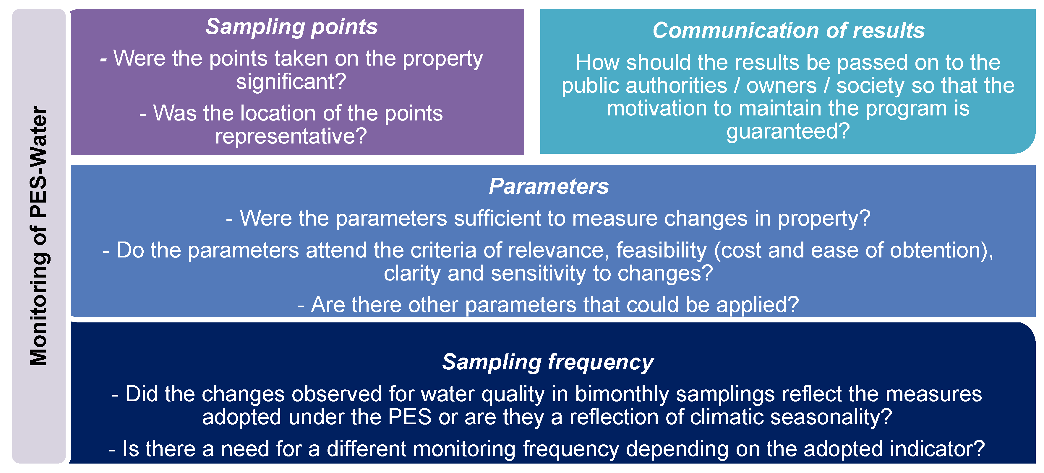
3.4. PES-Water Monitoring Program Proposal

Figure 4 presents guiding questions based on the document guide book for payment for environmental water services on area selection and monitoring [38], and the answers that are given to these questions in Figure 5 are based on results obtained in this study.

Knowing that water quality is influenced by the dynamics of climatic seasonality, and in the case of properties participating in the PES-Water program, related to changes in land use addressed through improvements, it is suggested that the monitoring frequency should be comprehensive and continuous. Furthermore, it should consider at least one hydrological year, which means that the indicators related to water quality are monitored twice a year, in the dry and rainy seasons. This climatic differentiation between the samplings is important to prevent possible changes in the monitored parameters being attributed to the interventions undertaken within the scope of the PES, since it is known that these can take years to be notified.

4. Discussion

4.1. Spatial–Temporal Variation of Water Quality Indicators

The occurrence of high values and absence of behavioral differentiation for the parameter of total coliforms at the sampling points is notable. The microbiological quality of natural waters tends to be compromised by the absence of plant protection that would act as a barrier for runoff, which can carry animal or even human feces and contain multi-resistant bacteria that cause contamination of the water resource [39]. However, the presence of the total coliforms in natural waters does not necessarily imply contamination by fecal material, since this group of coliforms includes bacteria that naturally occur in soils, water, and plants, especially in tropical climates; therefore, this is a limited health value analysis [40].

The water analysis from a spring in the rural area of the municipality of Varre-Sai, Rio de Janeiro, showed contamination by total coliforms in samples with a maximum of 1600 NMP/100 mL [41]. This contamination is associated with land use and occupation and is aggravated by precipitation events. A study of the microbiological quality of the water used for human consumption in the extreme western region of Santa Catarina observed that 64.1% of the analyzed samples were contaminated by total coliforms, highlighting the need to take preventive measures and properly treat compromised waters to prevent the occurrence of waterborne diseases [42].

A study from urban water bodies observed that the first component (33.4% of the total variance) was strongly associated with pH and turbidity, indicating that these variables are the most significant in defining the quality of water and moderately associated with thermotolerant coliforms and total residue. The second component (32.5%) was strongly associated with BOD, total phosphorus, and dissolved oxygen, and moderately associated with chlorophyll-a and total nitrogen. This can be interpreted as the influence of pollution sources that deposit nutrients in water bodies and generate eutrophication [43].

The observation that the results obtained in the factor analysis indicated that the parameters responsible for fluctuations in water quality was mainly related to the discharge of effluents and natural temperature so that in relatively less polluted areas there was contamination by a point source of domestic sewage. In areas of medium pollution, organic contamination came from a point source of domestic wastewater and nutrients from agriculture and orchard plantations, and in highly polluted areas the contamination came from point sources via domestic wastewater, wastewater treatment plants, and industries [44].

4.2. Spatial Variation of Soil Properties and Vegetation Cover

There is a direct relationship between soil pH and base saturation—V—so that the higher the pH, the higher the V%, confirming the one found in the study in ref. [45]. However, as described by the same author, soils with a very acidic pH, generally less than 4.5, tend to have phosphorus deficiency, low levels of Ca, Mg, and K, a good availability of iron, copper, manganese, and zinc micronutrients, low effective CEC, and base saturation, contrary to what was observed for the present study.

It is observed that points 2 (native forest) and 3 (sewer amount) had the lowest recorded levels of organic matter, since they are composed mainly of sand particles, with a percentage greater than 75% in both. Sandy soils tend to have a low content of organic matter and consequently a low average CEC, retaining small amounts of cations and therefore being more susceptible to nutrient loss [45].

In the analysis of the leaf area index (LAI), the highest value was recorded for point 7—2.817 m²/m², and the lowest value was recorded for point 5—0.325 m²/m², reflecting the conditions of use and occupation around them. According to the scale proposed [29], of the total sampled points, 42.8% depict LAI as referring to exposed soil (points 2, 3, and 5), 14.3% represents an area of exposed soil covered by undergrowth (point 6), 14.3% depicts an area with tree–shrub vegetation (point 1), and 28.6% represents an area with dense vegetation (points 4 and 7).

A study from Amazônas observed that the values for LAI vary depending on the ecosystem analyzed, as this indicator is influenced by the degree of soil fertility and water supply that establish the structure and floristic composition of the canopy [46]. The Ribeirão Anhumas Permanent Protection Area study in Campinas found that, in an area of urban influence, the LAI value varied between 1.311 m²/m² (dry) and 1.398 m²/m² (rain) and in a predominantly rural area, it varied between 1.548 m²/m² (dry) and 1.826 m²/m² (rain). Such values correlate with the values of organic matter and CEC of the soil so the lowest values for these indicators were obtained for the point located in an urban area and the highest values were obtained for the area of rural approximation [47].

4.3. Correlation between Water, Soil, and Vegetation Characteristics

Nutrients can be transferred from the tree biomass to the soil when the vegetation is washed by rain, which causes organic mineral substances to be dragged down, and via the decomposition of litter, leads to fallen trunks and branches, and dead roots. However, these events depend on the occurrence of rain, the temperature, and the leaf area index [48]. The organic matter from decomposed litter enables the nutrients to be incorporated in the soil, which adsorbs them through the CEC and the percentage of clay present in the samples [49].

Still, there is an influence of soil pH as well as sand content on the water parameters BOD, EC, and pH, such that the former reflects to a greater or lesser extent the water that drains over the soil surface or in its profile, mainly in erosion events. Erosion can take a greater amount of solids and sediments to the water bodies, including vegetation elements that have not yet degraded, and therefore increases the BOD rate and the electrical conductivity, and makes the pH more acidic. When only water quality parameters are analyzed, there is a low to medium correlation between the indicators, except for the total phosphorus and turbidity parameters that have a positive r of 0.79 and the TDS and pH parameters that have a 0.74 correlation.

4.4. PES-Water Monitoring Program Proposal

The results were obtained in this study through the field evaluation of the rural property participating in the PES, and the provisions of the legislation of National Water Agency (ANA). These include Resolution n° 903/2012, which creates the national surface water quality monitoring network, Resolution n° 357/2005 of the Environment National Council (CONAMA), which provides water quality standards and indexes, WQI—Water Quality Index, and TSI—Trophic State Index, that are commonly used to assess water quality. It is inferred that water monitoring must at the very least consider the dissolved oxygen parameters, electrical conductivity, temperature, turbidity, total dissolved solids, and total phosphorus. It is advisable that for the temperature parameter both the water temperature and the air temperature should be measured, to indicate any improvements in the microclimate resulting from the actions adopted under the program.

In addition, considering the objective of PES programs in ensuring water quality and quantity, it is suggested that a water flow/production indicator should be monitored and that precipitation on the property should be checked monthly. In practice, the results achieved by implementing public policies for PES on rural properties point to an increase in flow once conservation practices have improved. For example,

• The case of PES Curator of the Waters (Conservador das Águas) in Extrema (Brazil): in a publication referring to the program’s twelve years of existence, there are reports that in that period more than 1.3 million trees were planted and over 125 springs were protected, joining forces for the production of billions of liters of water [50];
• The reports of owners participating in the Oasis Apucarana (Oásis Apucarana) project in Paraná, who observed, after five years of implementation of the program in the municipality, the reappearance of springs thanks to the restoration of 64 ha of degraded areas and the protection of springs with fences to prevent cattle trampling on them [51];
• A study of the Guariroba basin in Campo Grande, Mato Grosso do Sul, which found that the environmental practices encouraged by the PES program Living Source (Manancial Vivo) provided an increase in the base flow, which supports the total flow throughout the year. Although a reduction of approximately 1 mm in monthly precipitation was reported in the period between 2012 and 2016, the authors found an increase in the base flow of approximately 0.018 m³/s [52].

Regarding the monitoring of the environmental conditions in the areas covered by the analyzed points, with the monitoring of the soil it was noted that the survey carried out at the sampling points showed little difference in fertility between them. Although they are treated secondarily in PES-Water programs, soil quality indicators are essential in the study of programs with a water focus to check aspects related to erosion and also the soil’s edaphic conditions for plant growth. Parameters such as organic matter, CEC, macro- and micro-nutrients, despite being influenced by the vegetation decomposition in the soil, can be evaluated annually [53,54].

As for vegetation, changes resulting from forest restoration or conservation are usually slow and therefore need to be more widely monitored. This type of information is associated with the availability of satellite images. Thus, the percentage of vegetation cover can be monitored every two years. However, practices aimed at forest recovery such as area fencing, seedling production, planting, and enrichment can be monitored every six months.

In PES programs with a water focus, the maintenance of vegetation cover, especially on agricultural land, is of paramount importance as it protects the soil from the direct action of precipitation and increases the infiltration of water into the soil [55]. Starting from the idea that the PES-Water schemes are also aimed at controlling erosion and/or regulating water flow, vegetation provides the services for regulating water flow, controlling water quality, and soil protection [56]. Therefore, a synthesis of the proposed PES monitoring implementation is presented in Figure 6.

The results of the monitoring should be systematized to mainly address the advances made from implementing the program. They should be disseminated and made available clearly and directly, with an accessible and easily understood vocabulary, either to the general public or to the owners. This can be carried out via meetings, events, and websites, respecting the principle of transparency and publicity, especially where the service provider is concerned. It is also suggested that explanatory booklets about the PES could be prepared and made available to owners and users of the watershed.

Furthermore, technical training actions (lectures, courses, meetings, and seminars) can be developed with a view to improving understanding of the PES instrument, and involving managers, technicians, beneficiaries, providers, and payers of environmental services. It is essential that service providers are engaged and motivated so that they can see themselves as a basic part of the program from its conception and participate more actively on their property, so that they feel comfortable suggesting actions and solutions.

5. Conclusions

The establishment of a monitoring system is a key issue for the success of a PES initiative. It requires a precise definition of parameters to be evaluated in all the elements that are considered (environmental, economic and social). These parameters should be defined ex ante, in the planning stage of the program, to prevent conflicts due to changes in the evaluation criteria after the properties are enrolled.

The results showed that water quality indicators are independent of spatial–temporal variability, so that, for the parameters of DO, BOD, pH, TP, and TN, a greater oscillation was observed relative to the spatial location of the sample points, and for the parameters of turbidity, temperature, and EC, there was greater change between samplings. Such sample heterogeneity was borne out by the applied statistical analysis; the multivariate PCA analysis showed that the indicators that stood out were turbidity and temperature associated with point 6 (livestock interference), pH with points 1 (downstream property), 3 (sewer amount) and 5 (consumption—nascent), TP with points 2 (native forest) and 6 (livestock interference), and DO and EC in point 1 (Downstream property) and point 2 (native forest). In the analysis of the correlation between the physical–chemical parameters of the soil, LAI, and water quality indicators, there was a medium to high correlation among the soil quality indicators, especially regarding the content of MO and nutrients. When analyzing only the parameters of water quality, there was a low to medium correlation between the indicators, except for the parameters TP–turbidity, and TDS–pH. Based on the results we can conclude that the list of indicators analyzed can support PES program monitoring in Brazil. Additionally, the methodology developed can be easily applied in other areas and provide the definition of the most suitable indicators to monitor water-based PES in different Brazilian contexts.

References

1. Farley, J.; Costanza, R. Payments for ecosystem services: From local to global. Ecol. Econ. 2010, 69, 2060–2068. [Google Scholar] [CrossRef]
2. Gutman, P. Ecosystem services: Foundations for a new rural–urban compact. Ecol. Econ. 2007, 62, 383–387. [Google Scholar] [CrossRef]
3. Díaz, S.; Demissew, S.; Carabias, J.; Joly, C.; Lonsdale, M.; Ash, N.; Larigauderie, A.; Adhikari, J.R.; Arico, S.; Báldi, A.; et al. The IPBES conceptual framework—Connecting nature and people. Curr. Opin. Environ. Sustain. 2015, 14, 1–16. [Google Scholar] [CrossRef] [Green Version]
4. IUCN. Facilitating Conservation through the Establishment of Protected Areas as a Basis for Achieving Target 11 of the Strategic Plan for Biodiversity 2011–2020; IUCN: Gland, Switzerland, 2010. Available online: https://portals.iucn.org/library/sites/library/files/resrecfiles/WCC_2012_RES_35_EN.pdf (accessed on 13 November 2020).
5. European Commission. Our Life Insurance, Our Natural Capital: An EU Biodiversity Strategy to 2020; European Commission: Brussels, Belgium, 2011. [Google Scholar]
6. Executive Office of the President of the United States. Incorporating Ecosystem Services into Federal Decision Making; (M-16-01); US Government: Washongton, DC, USA, 2015.
7. Campanha, M.M.; Pedreira, B.C.C.G.; Fidalgo, E.C.C.; Parron, L.M.; Prado, R.B.; Bergier, I.; Monteiro, J.M.G.; Ferraz, R.P.D.; Turetta, A.P.D.; Tonucci, R.G.; et al. Serviços ecossistêmicos: Histórico e evolução. In Marco Referencial em Serviços Ecossistêmicos; Embrapa: Brasília, Brazil, 2019; pp. 37–58. [Google Scholar]
8. Pan, X.; Xu, L.; Yang, Z.; Yu, B. Payments for ecosystem services in China: Policy, practice, and progress. J. Clean. Prod. 2017, 158, 200–208. [Google Scholar] [CrossRef]
9. Taffarello, D.; Srinivasan, R.; Mohor, G.S.; Guimarães, J.L.B.; do Carmo Calijuri, M.; Mendiondo, E.M. Modeling freshwater quality scenarios with ecosystem-based adaptation in the headwaters of the Cantareira system, Brazil. Hydrol. Earth Syst. Sci. 2018, 22, 4699–4723. [Google Scholar] [CrossRef] [Green Version]
10. Wunder, S.; Engel, S.; Pagiola, S. Taking stock: A comparative analysis of payments for environmental services programs in developed and developing countries. Ecol. Econ. 2008, 65, 834–885. [Google Scholar] [CrossRef]
11. Bernardes, A.C. Pagamento por serviços ambientais: Experiências brasileiras relacionadas à água. Encontro Nac. Anppas 2010, 5, 4–7. [Google Scholar]
12. Reed, M.S.; Moxey, A.; Prager, K.; Hanley, N.; Skates, J.; Bonn, A.; Evans, C.D.; Glenk, K.; Thomson, K. Improving the link between payments and the provision of ecosystem services in agri-environment schemes. Ecosyst. Serv. 2014, 9, 44–53. [Google Scholar] [CrossRef] [Green Version]
13. Calvet-Mir, L.; Corbera, E.; Martin, A.; Fisher, J.; Gross-Camp, N. Payments for ecosystem services in the tropics: A closer look at effectiveness and equity. Curr. Opin. Environ. Sustain. 2015, 14, 150–162. [Google Scholar] [CrossRef] [Green Version]
14. Ola, O.; Menapace, L.; Benjamin, E.; Lang, H. Determinants of the environmental conservation and poverty alleviation objectives of Payments for Ecosystem Services (PES) programs. Ecosyst. Serv. 2019, 35, 52–66. [Google Scholar] [CrossRef]
15. Lima, A.P.M.; Prado, R.B.; Schuler, A.E.; Fidalgo, E.C.C. Metodologias de monitoramento de Programas de Pagamento por Serviços Ambientais Hídricos no Brasil. In Simpósio Brasileiro de Recursos Hídricos; Associação Brasileira de Recursos Hídricos: Porto Alegre, Brazil, 2015. [Google Scholar]
16. Llambí, L.; Becerra, M.T.; Peralvo, M.; Avella, A.; Baruffol, M.; Díaz, L.J. Monitoring biodiversity and ecosystem services in Colombia’s High Andean Ecosystems: Toward an integrated strategy. Mt. Res. Dev. 2020, 39, 8–20. [Google Scholar] [CrossRef] [Green Version]
17. Martínez, R.Q. Guía Metodológica Para Desarrollar Indicadores Ambientales y de Desarrollo Sostenible em Países de América Latina y el Caribe; CEPAL: Santiago, Chile, 2009; 130p. [Google Scholar]
18. Young, C.E.F.; Bakke, R.L.B. Payments for ecosystem services from watershed protection: A methodological assessment of the oasis project in brazil. Nat. Conserv. 2014, 12, 71–78. [Google Scholar] [CrossRef] [Green Version]
19. Balvanera, P.; Quijas, S.; Karp, D.S.; Ash, N.; Bennett, E.M.; Boumans, R.; Brown, C.; Chan, K.M.A.; Chaplin-Kramer, R.; Halpern, B.S.; et al. Ecosystem Services. In The GEO Handbook on Biodiversity Observation Networks; Springer: Cham, Switzerland, 2017. [Google Scholar]
20. Cord, A.F.; Brauman, K.A.; Chaplin-Kramer, R.; Huth, A.; Ziv, G.; Seppelt, R. Priorities to Advance Monitoring of Ecosystem Services Using Earth Observation. Trends Ecol. Evol. 2017, 32, 416–428. [Google Scholar] [CrossRef] [PubMed]
21. Martin-Ortega, J.; Ojea, E.; Roux, C. Payments for Water Ecosystem Services in Latin America: A literature review and conceptual model. Ecosyst. Serv. 2013, 6, 122–132. [Google Scholar] [CrossRef]
22. Chen, H.L.; Lewison, R.L.; An, L.; Tsai, Y.H.; Stow, D.; Shi, L.; Yang, S. Assessing the effects of Payments for Ecosystem Services programs on forest structure and species biodiversity. Biodivers. Conserv. 2020, 29, 2123–2140. [Google Scholar] [CrossRef] [Green Version]
23. Lima, G. Aplicação de Simulação Computacional na Análise dos Conflitos Entre os Usos Múltiplos da Água na Bacia do Rio Atibaia no Estado de São Paulo. Master’s Thesis, Universidade de São Paulo, São Carlos, Brazil, 2002. [Google Scholar]
24. Oliveira, F.L. A Percepção Climática No Município de Campinas-SP. Master’s Thesis, Universidade Estadual de Campinas, Campinas, Brazil, 2005. [Google Scholar]
25. CIIAGRO. Centro Integrado de Informações Agrometeorológicas. Available online: http://www.ciiagro.sp.gov.br/ciiagroonline/ (accessed on 20 October 2020).
26. Baio, F.H.R.; da Silva Faraun, R.; Teodoro, P.E.; da Silva, A.F.; Neves, D.C.; Azevedo, G.B. Correlations and Principal Components Analysis for Defining Management Zones in Cotton. Braz. J. Dev. 2020, 6, 7393–7407. [Google Scholar] [CrossRef]
27. Raij, B.; Andrade, J.C.; Cantarella, H.; Quaggio, J.A. Análise Química Para Avaliação da Fertilidade de Solos Tropicais; Instituto Agronômico: Campinas, Brazil, 2001; 285p. [Google Scholar]
28. Galvani, E.; Lima, N.G.B. Fotografias hemisféricas em estudos microclimáticos: Referencial teórico-conceitual e aplicações. Ciência Nat. 2014, 36, 215–221. [Google Scholar] [CrossRef] [Green Version]
29. Oliveira, T.H.; Oliveira, J.S.; Machado, C.C.; Rodrigues, G.T.; Galvíncio, J.D.; Pimentel, R.M. Avaliação espaço-temporal do Índice de área foliar e impacto das atividades antrópicas na Reserva Ecológica Estadual Mata São João da Várzea, Recife—PE. Simpósio Bras. Sens. Remoto 2011, 15, 2105–2112. [Google Scholar]
30. Figueiredo Filho, D.B.; Silva Júnior, J.A. Desvendando os mistérios do coeficiente de correlação de Pearson. Rev. Política Hoje 2009, 18, 115–146. [Google Scholar]
31. Paranhos, R.; Figueiredo Filho, D.B.; da Rocha, E.C.; da Silva Júnior, J.A.; Neves, J.A.B.; Santos, M.L.W.D. Desvendando os Mistérios do Coeficiente de Correlação de Pearson: O Retorno. Leviathan 2014, 8, 66–95. [Google Scholar] [CrossRef] [Green Version]
32. Vicini, L. Análise Multivariada da Teoria à Prática; Monografia; Especialização em Estatística e Modelagem Quantitativa, Universidade Federal de Santa Maria: Santa Maria, Brazil, 2005. [Google Scholar]
33. Liu, C.W.; Lin, K.H.; Kuo, Y.M. Application of factor analysis in the assessment of groundwater quality in a Blackfoot disease área in Twain. Sci. Total Environ. 2003, 313, 77–89. [Google Scholar] [CrossRef] [PubMed]
34. Medeiros, G.A.; Tresmondi, A.C.C.L.; Queiroz, B.P.V.; Fengler, F.H.; Rosa, A.H.; Fialho, J.M.; Lopes, R.S.; Negro, C.V.; Santos, L.F.; Ribeio, A.I. Water quality, pollutant loads, and multivariate analysis of the effects of sewage discharges into urban streams of Southeast Brazil. Energ. Ecol. Environ. 2017, 2, 259–276. [Google Scholar] [CrossRef] [Green Version]
35. Ouyang, Y. Evaluation of river water quality monitoring stations by principal component analysis. Water Res. 2005, 39, 2621–2635. [Google Scholar] [CrossRef] [PubMed]
36. Ronquim, C.C. Conceitos de Fertilidade do Solo e Manejo Adequado Para as Regiões Tropicais; EMBRAPA Monitoramento por Satélite: Campinas, Brazil, 2010; 26p. [Google Scholar]
37. Salvador, J.O.; Moreira, A.; Malavolta, E. Cleusa Pereira Cabral, C.P. Boron and manganese influence on growth and mineral composition on young guava plants. Ciência Agrotecnol. 2003, 27, 325–331. [Google Scholar] [CrossRef]
38. Fidalgo, E.C.C.; Prado, R.B.; Turetta, A.P.D.; Schuler, A.E. Manual para Pagamento por Serviços Ambientais Hídricos: Seleção de Áreas e Monitoramento; Embrapa: Brasília, Brazil, 2017. [Google Scholar]
39. Bortoloti, K.C.S.; Melloni, R.; Marques, P.S.; de Carvalho, B.M.F.; Andrade, M.C. Microbiological quality of natural waters on the resistance profile of heterotrophic bacteria to antimicrobials. Eng. Sanitária Ambient. 2018, 23, 717–725. [Google Scholar] [CrossRef]
40. Brasil Ministério da Saúde; Secretaria de Vigilância em Saúde. Inspeção Sanitária em Abastecimento de Água; Série A: Normas e Manuais Técnicos; Ministério da Saúde: Brasília, Brazil, 2007. [Google Scholar]
41. Santos, E.P.P.; Veiga, W.A.; Gonçalves, M.R.S.; Thomé, M.P.M. Coliformes Totais e Termotolerantes em água de nascentes utilizadas para o consumo humano na zona rural do município de Varre-Sai, RJ. Sci. Plena 2015, 11, 052401. [Google Scholar]
42. Scapin, D.; Rossi, E.M.; Oro, D. Microbiological quality of water used for human consumption in the extreme western region of Santa Catarina, Brazil. Rev. Inst. Adolfo Lutz 2012, 71, 593–596. [Google Scholar]
43. Silva, C.O.F.; Goveia, D. Evaluation of environmental quality of urban water bodies using multivariate analysis. Interações 2019, 20, 947–958. [Google Scholar] [CrossRef]
44. Shrestha, S.; Kazama, F. Assessment of surface water quality using multivariate statistical techniques: A case study of the Fuji River basin, Japan. Environ. Model. Softw. 2007, 22, 464–475. [Google Scholar] [CrossRef]
45. Villar, M.L.P. Manual de Interpretação de Análise de Plantas e Solos e Recomendação de Adubação; EMPAER: Cuiabá, Brazil, 2007; 182p. [Google Scholar]
46. Villani, F.T. Dinâmica da Matéria orgânica e Fertilidade do Solo em Sistemas Agroflorestais e Outras Coberturas Vegetais em Comunidades Indígenas do Alto Solimões Amazonas. Ph.D. Thesis, Federal University of Amazonas, Manaus, Brazil, 2009. [Google Scholar]
47. Garcia, J.M.; Longo, R.M. Análise de impactos ambientais em Área de Preservação Permanente (APP) como instrumento de gestão em rios urbanos. Cerrados 2020, 18, 107–128. [Google Scholar] [CrossRef]
48. Bambi, P. Variação Sazonal do Índice da Área Foliar e Sua Contribuição na Composição da Serapilheira e Ciclagem de Nutrientes na Floresta de Transição no Norte do Mato Grosso. Master’s Thesis, Universidade Federal de Mato Grosso, Cuiabá, Brazil, 2007. [Google Scholar]
49. Pedralino, F.O.; Barbosa, B.S.; Cabral, I.F.; Souza, L.A.C.; Coringa, E.A.O. Indicadores ambientais de solos do Instituto Federal de Mato Grosso, Campus Cuiabá-Bela Vista. In Proceedings of the Congresso Brasileiro De Gestão Ambiental, 2013; IBEAS: Salvador, Brazil, 2013; Volume 4. [Google Scholar]
50. Pereira, P.H. Conservador das Águas: 12 Anos; Prefeitura de Extrema, Secretaria Municipal de Meio Ambiente: Extrema, Brazil, 2017. [Google Scholar]
51. Pagiola, S.; Von Glehn, H.C.; Taffarello, D. Experiências de Pagamentos por Serviços Ambientais no Brasil; SMA/CBRN: São Paulo, Brazil, 2013. [Google Scholar]
52. Sone, J.S.; Gesualdo, G.C.; Zamboni, P.A.P.; Vieira, N.O.M.; Mattos, T.S.; Carvalho, G.A.; Rodrigues, D.B.B.; Sobrinho, T.A.; Oliveira, P.T. Water provisioning improvement through payment for ecosystem services. Sci. Total Environ. 2019, 655, 1197–1206. [Google Scholar] [CrossRef] [PubMed]
53. Carneiro, M.A.C.; de Souza, E.D.; dos Reis, E.F.; Pereira, H.S.; de Azevedo, W.R. Physical, chemical and biological properties of cerrado soil under different land use and tillage systems. Rev. Bras. Ciência Solo 2009, 33, 147–157. [Google Scholar] [CrossRef] [Green Version]
54. Portugal, A.F.; Juncksh, I.; Schaefer, C.E.; Neves, J.C.L. Aggregate stability in an ultisol under different uses, compared with forest. Rev. Ceres 2010, 57, 545–553. [Google Scholar] [CrossRef] [Green Version]
55. Favaretto, N.; Cogo, N.P.; Bertol, O.J. Uso, manejo e conservação do solo e da água: Aspectos agrícolas e ambientais. In Diagnóstico e Recomendações de Manejo do Solo: Aspectos Teóricos e Metodológicos; UFPR/Setor de Ciências Agrarias: Curitiba, Brazil, 2006; pp. 293–341. [Google Scholar]
56. Guedes, F.B.; Seehusen, S.E. Pagamentos por Serviços Ambientais na Mata Atlântica: Lições Aprendidas e Desafios; MMA: Brasília, Brazil, 2011. [Google Scholar]
Figure 1. Location of the study area in the city of Campinas and state of São Paulo, Brazil.
Sustainability 15 09593 g001
Figure 2. PCA factor load: (a) April 2019, (b) July 2019, (c) September 2019, (d) November 2019, (e) January 2020. F1 and F2-components; DO-dissolved oxygen, BOD-biochemical oxygen demand, Turb-turbidity, Temp-temperature, EC-electrical conductivity, TDS-total dissolved solids, TP-total phosphorus, and TN-total nitrogen. Black circles-association with F1 (Component 1) and gray circles-association with F2 (Component 2).
Sustainability 15 09593 g002
Figure 3. Correlation matrix between water, soil, and vegetation properties in the selected main components. Blue cells-negative correlation, red cells-positive correlation. Veg-vegetation, P-phosphorus, OM-organic matter, pHS-soil pH, Ca-calcium, Mg-magnesium, H + Al-total acidity, CEC-cation exchange capacity, V%-base saturation, B-boron, Cu-copper, Fe-iron, Mn-manganese, Zn-zinc, LAI-leaf area index, DO-dissolved oxygen, BOD-biochemical oxygen demand, pHA—water pH, Turb—turbidity, Temp—temperature, EC—electrical conductivity, TDS-total dissolved solids, TP-total phosphorus, and TN-total nitrogen. R coefficient between 0.10 and 0.30: weak correlation; r coefficient between 0.40 and 0.60: moderate correlation; r coefficient between 0.70 to 1: strong correlation.
Sustainability 15 09593 g003
Figure 4. Guiding questions for implementing PES-Water monitoring.
Sustainability 15 09593 g004
Figure 5. Basic responses for the implementation of PES-Water monitoring.
Sustainability 15 09593 g005
Figure 6. Implementation flowchart of the PES-Water monitoring program.
Sustainability 15 09593 g006