Article

Sustainable Development between Demonstration Farm and Agricultural Labor Productivity: Evidence from Family Farms in the Mountainous Area of Western China

1
School of Public Policy and Management, Guangxi University, Nanning 530004, China
2
School of Economics and Management, Tongren University, Tongren 554300, China
3
Chongqing Academy of Social Sciences, Chongqing 400020, China
4
School of Economics and Management, Southwest University, Chongqing 400715, China
*
Authors to whom correspondence should be addressed.
Sustainability 2023, 15(12), 9560; https://doi.org/10.3390/su15129560
Submission received: 7 March 2023 / Revised: 30 May 2023 / Accepted: 2 June 2023 / Published: 14 June 2023
(This article belongs to the Special Issue Sustainable Agricultural Economy)

Abstract

:
Agricultural labor productivity is an important indicator that reflects the sustainable development of agriculture and rural areas. Demonstration farms provide an important link between small-scale farmers and modern agriculture in mountainous area of western China, which is playing an important role in improving labor productivity. This paper focuses on using the PSM-logit model and sensitivity analysis to empirically test the causal relationship between demonstration farms and labor productivity, and a micro-large sample of 1823 family farms was adopted. The highlighted findings are as follows: the average labor productivity of the demonstration farm is 2.8 times higher than that of the non-demonstration farm. There is a significant positive correlation between demonstration farms and labor productivity. Utilizing demonstration farms, when all control variables are added, can remarkably promote farm income by CNY301458 on average. In the matched sample, and under scenarios controlling for other covariates, we saw that demonstration farms can significantly enhance the farm income of CNY285108, CNY288509, and CNY291077 on average, respectively, after taking the radius matching, the kernel matching, and the nearest neighbor matching. The research inspired us to enhance the demonstrative establishment of family farms and accelerate the rate at which comprehensive development benefits are derived from demonstration farms. The results of this research could provide a policy reference for the promotion of high-quality development and the sustainable development of family farms in China and serve as an experience reference for promoting sustainable development of agriculture and rural areas globally.

1. Introduction

Improving agricultural labor productivity is an important symbol of realizing agricultural modernization [1,2]. First, it directly means increasing farm income, which is conducive to promoting the sustainable development of the agricultural economy. Secondly, it can drive farm employment, which is conducive to promoting the sustainable development of agricultural society. At the same time, the green development of agriculture also imposes new requirements on the improvement of labor productivity, which will also be conducive to indirectly promoting sustainable development of agricultural ecology. Family farms are the basis for the functioning of agricultural sectors in many regions of the world [3] and also serve as an important link between small-scale farmers and modern agriculture in China, especially in the western mountainous areas. The originally intent behind establishing demonstration family farms is to improve agricultural labor productivity, which has important and long-term significance in promoting agricultural and rural modernization and promoting the common prosperity of farmers and rural areas [4]. Family farms can effectively extend industrial chains, expand supply chains and improve value chains, which plays an important role in helping to eliminate poverty and assisting farmers to raise their income [5,6], and it has gradually developed into the important approach of promoting agricultural and rural modernization [7,8]. The Communist Party of China (CPC) have always insisted on solving the problems of agriculture, rural and farmers as the top priority of all developmental work [5]. The implementation of the family contract responsibility system promotes the development of the rural economy in China. However, with the development of the historical process, some problems have been exposed, such as small scale of agricultural management, scattered management, backward agricultural technology and low production efficiency [9,10,11], which make it difficult to elevate the improvement of agricultural labor productivity. Therefore, it is extremely important to find an effective business model that can not only effectively compensate for the shortcomings of traditional small-scale farmer management, but also promote the moderate-scale management of land.
In China, the No. 1 central document of the CPC Central Committee first saw the phrase “family farm” written in as the new type agricultural business entities in 2013 [12]. Since then, there has been an emphasis on strongly supporting family farm development [12,13,14,15,16,17,18,19,20], which has become an important topic of discussion in the political and academic circles. A series of family farms demonstration cases have been established and popularized [21]. This initiative is an important channel for the improvement of labor productivity and an important experience in promoting the revitalization of the rural industry. Mountainous areas in western China are the key support areas for the realization of agricultural modernization and sustainable development. In this paper, Tongren city, with the geographic structure characteristic of the western mountain region [4], is selected as the study area. An empirical test on the causal relationship between demonstration farms and agricultural labor productivity, with a micro-large sample of 1823 family farms and PSM-logit model, is adopted. Additionally, this article attempts to answer the following three questions: (1) What is the labor productivity level on family farms in the mountainous area of western China? (2) Can demonstration farms improve labor productivity? (3) How much room is there for demonstration farms to contribute to improving labor productivity?
The highlights several innovations of this paper are summarized as follows: Firstly, this paper researches the effects of demonstration farm on labor productivity, which has important and far-reaching theoretical value and practical significance for promoting the connection between small-scale farmers and modern agriculture. Secondly, we select Tongren city as the research area. This site has mountainous geographic characteristics and green ecological advantages [4]. Located in the mountainous area of western China, the area has special value and representational significance. Thirdly, we focus on matching two groups of samples, namely, demonstration farm and non-demonstration farm by propensity score matching (PSM) method, and then calculating the average treatment effect of the matched sample, further examines the sensitivity of PSM estimation results to “hidden bias”. Based on the above innovations, the main academic contributions of this paper can be summarized as follows. The study is not only helpful in that it provides an effective development path for small-scale farmers in mountainous area to increase their income and become wealthy, but also helpfully provides an empirical basis and experiential reference for the development of modern agriculture in China. Finally, it is helpful as it provides a typical case in China for other countries or regions to use for the promotion of sustainable agricultural development.
The rest of the paper is structured as follows. Section 2 provides a literature review. Section 3 proposes a Theory and Method. Section 4 describes the Variables and Data. Section 5 details the Results and Discussions. Section 6 summarizes the Conclusions and Implications of this paper.

2. Literature Review

If a researcher looks extensively at the relevant theoretical research and academic exploration in policy and academic circles, they will find that the existing literature mainly comprises relatively rich research into the connotation and extension of family farm, the development of driving forces and factors, the development of efficiency and benefits, and the development of a path and policy proposal for improving labor productivity in family farm. This content lays a solid logical foundation for the research ideas and contents of this paper.
In the literature, there are numerous studies on the problems of connotation and extension of family farms. The development of family farms in Brazil [22,23], the Netherlands [24,25], France [26,27], Japan [28,29] and other countries has achieved good results, and the systems and mechanisms used are relatively perfect. The operation mode of first using a pilot and then promoting the system has been adopted in China, and a series of typical cases of family farm development have emerged [30,31,32,33,34,35]. Most studies fully indicate that family farms play outstanding roles and have obvious effect [5,6,7,35,36,37]. They also show the following remarkable characteristics centrally, such as family management, specialized division of labor, socialized cooperation, use of modern technology, enterprise operation, modern farming, market-oriented practice, agricultural commercialization, agricultural mechanization, green management, labor stability, and being agricultural income-oriented, etc. [38,39].
The subject of the development driving force and the influencing factors of labor productivity of family farms has attracted a great deal of attention and discussion from academic circles. In general, the development process of family farms is a process of continuously improving labor productivity to improve production power and grant the comparative advantages of low labor supervision cost, good scale benefit, high production efficiency, etc. [5,6,7,35,36,37]. Notwithstanding, the economic, social and ecological benefits of family farms can also be disturbed by various influencing factors [6,7,35,36,37,40,41]. For instance, mechanisms and tools of agricultural policy, agricultural mechanization, crop establishment, wage labor, quality capabilities of agricultural managers, level of internal management, rural financial credit system, satisfaction of social service demand, support for agricultural science and technology, and quality and safety of agricultural products, etc. [40,41,42,43,44,45,46]. As it should be, objectively speaking, the development of family farms in different countries and regions at different stages of development is affected by natural, social, economic, cultural, technical and other factors. Family farms also face many resource constraints.
There are many studies on the development efficiency and benefits of the labor productivity of family farms. Some scholars have reached relatively consistent conclusions. Some argue, for example, that welfare emerges as a legitimate element for the analysis of the family farm economy [47]; others assert that the larger the area of a small-scale family farm is, the greater its economic sustainability will be [46]. There is a positive correlation between the managing efficiency and economic benefits of family farms, and the management efficiency of family farms that adopt new technologies is relatively higher than that of family farms without new technologies [48]. The use of demonstration farms has a significant positive impact in terms of improving the develop benefits of family farms, increasing farm income, promoting the sustainable development of family farms, and enhancing the sense of the gain, happiness and security of farmers [6,7,35,36,37]. Of course, some scholars also found that the overall level of technical efficiency of Chinese family farms is relatively low and that the efficiency value is not high. There is a large room for improvement in both pure technical efficiency and scale-related efficiency [9,30].
There are also many scholars who have given constructive insights into the development path and policy recommendations for improving labor productivity in family farms. The development of family farms is a systematic, ecological, dynamic and sustainable process that needs to combine the internal force and external support of family farms organically [49]. Scholars should combine these policies with regional agricultural development, improve policy design for family farm development and popularize typical cases of demonstration farms [5,35,36]. We must establish and improve the efficiency improvement mechanisms and incentive and restraint system of demonstration farms [9]. We should cultivate new types of professional farmers [37], promote the integration of universities, enterprises and bases through “industry-university-research” cooperation [6], and cultivate demonstration farms with local characteristics [36]. At the same time, there is a need to improve farm infrastructure conditions, promote the rational allocation of resource elements, and strengthen agricultural green technology innovation and diffusion [50] in order to improve the labor productivity and economic sustainability of family farms [43], ensure the healthy and efficient development of family farms, and then accelerate the advancement of agricultural modernization [51].
In summary, the relevant research results at the domestic and foreign levels fully demonstrate the effectiveness and persistence of the demonstration farm, and various representative views provide rich theoretical support and empirical borrowing material for the research in this paper and lay the scientific research direction and idea framework. However, it is worth paying close attention to the fact that the following aspects of research are necessary to further deepen and expand our understanding in this area. This is also the unique feature of this paper.
Firstly, from a theoretical point of view, there is at present little to read literature when researching the causal effect of demonstration farm on labor productivity. This paper researches the effect of demonstration farms on labor productivity, a practice that has important and far-reaching theoretical value and practical significance for consolidating the family farm management system, promoting the connection between small-scale farmers and modern agriculture, increasing farm economic income, and advancing agriculture and rural sustainable development. This will also be the logical starting point of the strong argument presented in this paper.
Secondly, in the research into the existing literature on family farms, it can be observed that the eastern, northeastern and central parts of China are often selected as research areas. However, there is little literature on choosing western China as a representative area for research. This paper selects Tongren city as the research area. With mountainous geographic characteristics and green ecological advantages [4] in the mountainous area of western China, this area has special value and representational significance. It is beneficial to compare the heterogeneity of farm development in the western region with other regions, and also to provide typical cases of farm development for other countries or regions.
Thirdly, it can be seen from the research method used that the existing research on family farms mainly uses small sample analysis. For this reason, the micro-large sample data is adopted in this paper, that is, the empirical analysis based on the micro-large sample of 1823 family farms in the mountainous area of western China with relatively stronger reliability and validity is used. At the same time, this paper focuses on matching two groups of samples, namely, demonstration farms and non-demonstration farms via the PSM method, and then calculating the average treatment effect of the matched sample. In addition, this research further examines the sensitivity of PSM estimation results to “hidden bias”. This helps to avoid bias in the estimation results, which it is necessary to treat with the samples data before empirical research, due to the non-randomness of sample selection.

3. Theory and Method

3.1. Theoretical Mechanism

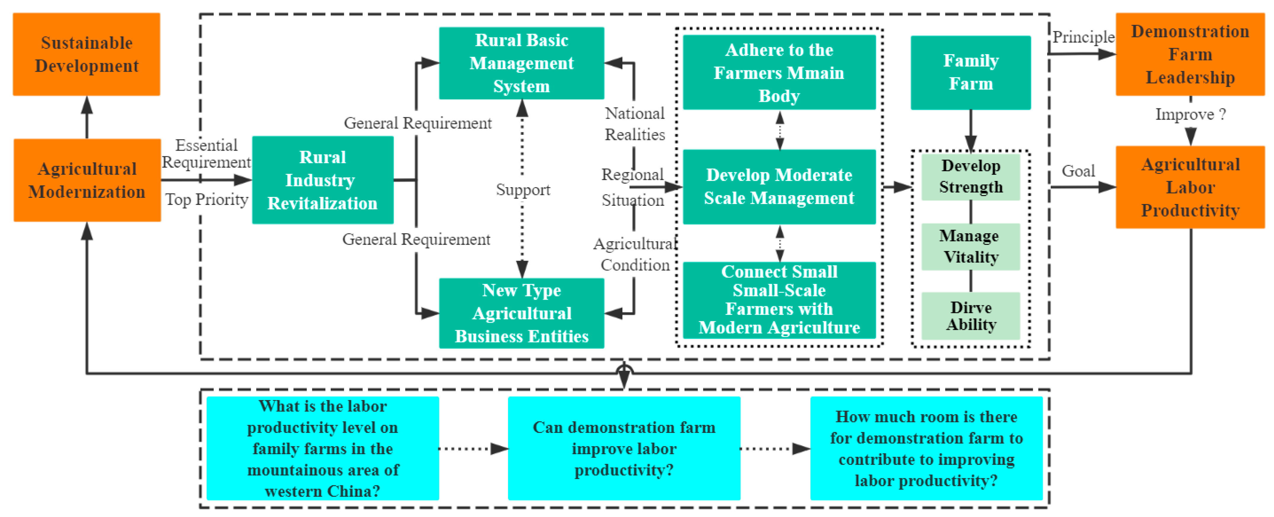
Reforming traditional agricultural theory [1] has played an important role as a theoretical basis supporting the process of promoting agricultural modernization in many countries. As an important component of the entire society, the agricultural industry not only provides development conditions for agricultural modernization, but also itself creates driving momentum for agricultural modernization [1], and its contributions, such as food, raw materials, markets, elements, and foreign exchange [2], have played indispensable and important roles in the process of agricultural modernization. Schultz [1] notes, however, that traditional agriculture in developing countries cannot contribute to economic growth, that only modern agriculture can make a significant contribution to economic growth, and that the key to the question is how to transform traditional agriculture into modern one. Furthermore, the question of how to transform weak traditional agriculture into a high-labor-productivity economic sector is also a central issue in transforming traditional agricultural theory. However, there are certain differences among different regions in China. For the mountainous area of western China, it is worth thinking about the kind of business entity that should be explored to improve agricultural labor productivity with adaptations to local conditions in the process of agricultural modernization. The theoretical mechanism for this paper is shown in Figure 1.
Firstly, transforming traditional agricultural industry implies the need to advance the revitalization of rural industry, which can neither be separated from the support force of the new type of agricultural business entities [5,6,7,35,36,37,51] nor from farmers, who occupy the primary position in this industry. Family farms in China mainly refer to the use of family members as the primary labor force and the family as the basic operational unit, and they are engaged in agriculturally scaled, standardized, and intensive production operations, which is the main business entity in modern agriculture [52]. Obviously, family farms are one of the best business entities to promote rural industry revitalization [5].
Secondly, family farms adhere to the rural basic management system and have played an important role as a booster in the process of agricultural modernization, and the issue of its scale is very noticeable in the theory of how to organize agricultural production. Schultz [1] suggests that we should not blindly establish large-scale farms, but rather create family farms that integrate ownership and management rights, adapt to market changes, and provide economic incentives and rewards for effective decision making. Clearly, Chinese family farms are an effective model for moderate-scale business.
Thirdly, there are still many small farmers in China, especially in western mountainous areas. Family farms are effective against the background of the realistic contradictions between and challenges of small-scale farming and modern agricultural development. Additionally, they serve to link these two issues. Comparatively speaking, the economic, social and ecological benefits of demonstration farms [6,7,9,35,36,37] are very significant.
Based on taking the above analyses together, we propose the following theoretical hypotheses.
Hypothesis 1.
The agricultural labor productivity level on family farms in the mountainous area of western China is uncertain.
Hypothesis 2.
Demonstration farms have a positive effect on agricultural labor productivity.
Hypothesis 3.
The room for demonstration farms to improve agricultural labor productivity is uncertain.

3.2. Method

First of all, the paper draws on the experience of the Rubin causal model (RCM, also known as a counterfactual framework) [53,54], which can reflect whether there is a causal effect of demonstration farms on labor productivity.
Based on whether or not a family farm is a demonstration farm, the treatment group (the treated group) and the comparison group (the control group) are composed. That is, the treatment variable D F i = 0 ,   1 . Among these values, “0” represents the demonstration farm, and “1” represents the non-demonstration farm. In this case, for a family farm sample i, there may be two states of the treatment variable DF on labor productivity (LP). These are as follows:
L P i =   L P 1 i   ,     i f     D F i = 1 L P 0 i   ,     i f     D F i = 0
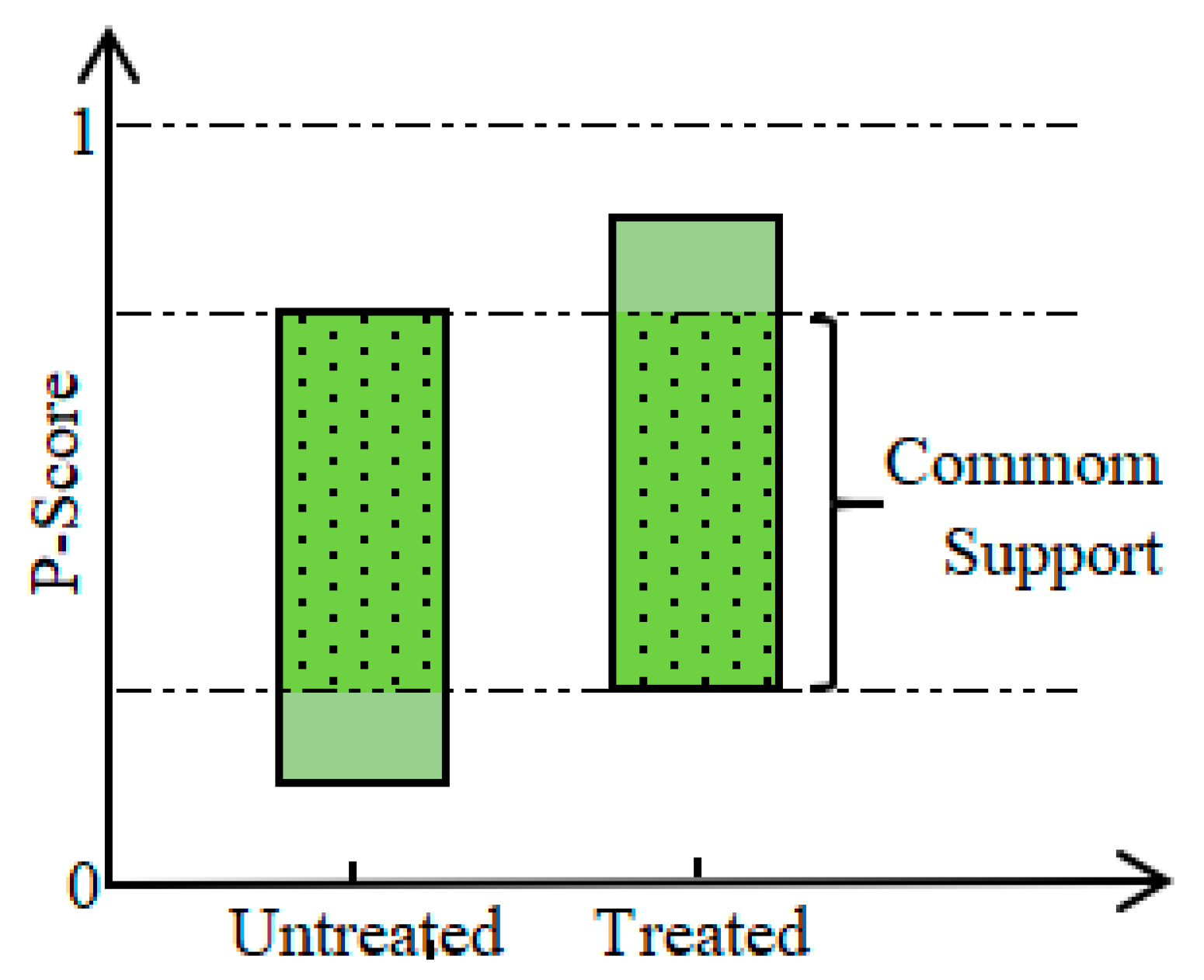
where L P i is the labor productivity of sample i, L P 1 i   is the labor productivity of sample i of demonstration farm,   and   L P 0 i is the labor productivity of sample i of non-demonstration farm. In order to ensure that the members in the sample can be matched, the matching assumption needs to be satisfied on each possible value of X i and ensure that the propensity score of the treatment group and control group share common support. For any value of X i , there exists 0 < P X i < 1 . The common support of the propensity score is clearly depicted in Figure 2.
Considering that the practice of establishing demonstration farms may be influenced by other factors, direct regression estimation may lead to biased empirical results. In view of this, firstly, the PSM method is used to search for control groups that are similar to those recognized as demonstration farms in order to eliminate the problem of sample selectivity so that the treated group and control group can have a common trend. Meanwhile, combining multiple logit models to estimate the true effects of the demonstration farm can ensure the accuracy and effectiveness of the empirical results to a large extent. The general steps [54,55] for calculating the average treatment effect using the PSM method are as follows.
Step 1: Select covariates. In order to ensure the quantity and quality of the selection of covariates and avoid bias, the relevant variables affecting L P 0 i   , L P 1 i and D F i should be taken into account as much as possible.
Step 2: Estimate propensity score. The purpose of estimating the propensity scores of the treatment group and the control group based on the logit regression model is to reduce the dimension of the multidimensional differences between the treatment group and the control group [35,54,55] so as to facilitate the subsequent matching of the propensity scores. This is shown in the Formula (2).
  P X i = P   D F i = 1     X i = e x p   β X i 1 + e x p   β X i
where X i is the covariates matrix, X i is the covariates vector, and P X i indicates the propensity score of the treatment group and the control group under the X i .
Step 3: Propensity score matching. According to the suggestions of scholars [35,54,55], the three most commonly used and popular matching methods are adopted in this paper, namely, the nearest neighbor matching within caliper, radius matching, and kernel matching methods.
The absolute distance of propensity score for radius matching is as follows.
D   P i = P 1 i P 0 j < ε
where P 1 i   and P 0 j   are the propensity score of the ith treatment group and the propensity score of the jth control group, respectively, and ε is the prior setting tolerance for matching. Generally speaking, caliper size uses a quarter of the standard deviation of the propensity score via sample estimates [35,54,55,56], that is, ε 0.25 σ p s c o r e   , σ p s c o r e is the standard deviation of the propensity score by sample estimates.
The absolute distance of propensity score for nearest neighbor matching within caliper is as follows.
D   P i =   j       m i n   P 1 i P 0 j < ε
The purpose of nearest neighbor matching within the caliper is to find the nearest matching within the given caliper range. Under normal circumstances, ε 0.25 σ p s c o r e   .
The weight expression of the propensity score for kernel matching is as follows.
W   i ,   j = K   X j X i h k   :   D k = 0   K   X j X i h    
where W     i ,   j is means the weight suitable for the matched   i ,   j , h is the bandwidth, and K( · ) is the kernel function.
Step 4: Balance test. The purpose of using the balance test on the matched samples is to ensure that there are no significant statistical differences in the covariates between the matched samples of treatment group and control group. It is generally calculated with the “standardized bias” of each covariate. The calculation is performed as shown in Formula (6).
X 1 ¯ X 0 ¯     V 1 X 2 + V 0 X 2   2  
where V 1 X 2 and V 0 X 2 are the sample variance of the covariates of treatment group and control group, respectively. It is generally required that the standardization difference should not exceed 10%. If it exceeds this value, the second or first step should be repeated until there is no significant difference.
Step 5: Calculate average treatment effect on the treated. The average treatment effect on the treated (ATT) is mainly calculated according to the matched sample in this paper. ATT formula is as follows.
A T T E   L P 1 i L P 0 i     D F i   = 1
The formula of estimator for average treatment effect on the treated is as follows.
A T T ^ = 1 N 1   i :   D F i   = 1 L P 1 i L P 0 i ^
where N 1 = i D F i   is individual number of the treatment group, and   i :   D F i   = 1   meant the total addition of individual number in the treatment group.
General steps of the propensity score matching is draw the outline of Figure 3.

4. Variables and Data

4.1. Variables Selection and Definition

Due to the difficulty of obtaining complete statistical data on variables, this paper draws on the research experience of other scholars for reference [6,7,35,36,37], considers the representativeness, availability and authority of the statistics, and follows the principles of consistency, integrity and scientificity of variables [4,57]. In view of these methods, which select the variables closely related to demonstration farms and the labor productivity of family farms, three classes of variable are included as follows. The settings and definitions of the variables are listed in Table 1.
(1) Dependent variable. Improving labor productivity is the core indicator of agricultural modernization. In real-life applications, promoting the improvement of agricultural labor productivity will contribute to raising the income of agricultural family laborers. This, in turn, promotes the sustainable development of family farms. In view of this, this paper sets the labor productivity (L.P.) as the outcome variable, which is the per capita production value of family farms.
(2) Core independent variable. From a practical point of view, when a family farm is established like a demonstration farm, it means that the farm has complete infrastructure, moderate large-scale management, scientific management, production standards and specifications, obvious demonstrations driving roles, etc. These measures mean that the productivity of the farm is higher than a certain probability of the average level of the whole city, meaning that the per capita income of the farm is higher than a certain ratio of the per capita income of local farmers. Thus, in relative terms, the more obvious the role of demonstration as a driving force is, the more it can actively drive the surrounding farmers to increase their income. Therefore, the demonstration farm (D.F.) is taken as the treatment variable.
(3) Control variable. In this paper, the following covariates that have a close relationship with outcome variable and treatment variable are also selected as control variables to reflect the basic situation of individual characteristics, labor input, operating conditions, experience accumulation, and agricultural environment of the family farm. Examples include head farmer gender (F.G.), head farmer age (F.A.), head farmer education (F.E.), family laborers (F.L_1), farm products (F.P.), farmland (F.L_2), management type (M.T.), management experience (M.E.), farm distance_county (D.C.), farm distance_town (D.T.), etc.

4.2. Data Interpretation and Source

Before introducing the data sources, it is necessary to define the family farm of this paper. The family farm selected in this paper mainly refers to a new type of agricultural business entity identified by the Agriculture and Rural Bureau of Tongren city that takes family members as the main labor force, agricultural income as the main source, and engages in moderate-scale, intensive and commercialized production and management of agricultural land. According to the geographic characteristics of the mountainous area in Western China, this territory mainly includes the following business types, including mountain planting type, dam land planting type, animal husbandry type, aquaculture type, and comprehensive planting and breeding type. Demonstration farms are established on the basis of encouraging farmers to operate independently, cultivated by the township government, recommended by the county government, and approved by the municipal government in areas where meet the conditions of moderate business scale, standardized farm business management, good and safe product quality, significant economies of scale, strong demonstration and driven benefits. Some of the variables were derived from the family farm statistics data of the Agriculture and rural Bureau of Tongren city. Data collection, sorting out and statistical analyses were carried out on some variables by the authors of this study based on the basic statistical data of Agricultural and Rural Bureau of Tongren city. The empirical data used are mainly from the 1823 family farms in Tongren city from 2013 to 2020.

4.3. Descriptive Statistics Analysis

The results of the descriptive statistics analysis of the variables are shown in Table 2. The statistical results of the mean, standard deviation, skewness, kurtosis, and number of samples from the control group and treated group are displayed in detail in the table, respectively. On the whole, the distribution of most variables is relatively concentrated, and the degree of dispersion is small. However, it is also found that the standard deviation of farm land (F.L_2), labor productivity (L.P.), farm distance_county (D.C.), and farm Distance_Town (D.T.) are relatively high, which shows that there are some differences between farm land, labor productivity, farm distance_county, and farm Distance_Town in the sample data to some extent. Meanwhile, farmland (F.L_2), labor productivity (L.P.), and farm distance_town (D.T.) have higher positive skewness and positive kurtosis, as the results show that there are many extreme values in the data series of the above variables, there are outlier data values, and the distance between the data and the mean value is relatively large. In addition, it is worth mentioning that the average labor productivity of the treated group is 2.8 times higher than that of the control group.

5. Results and Discussions

5.1. Correlation Analysis

The detailed changes of the correlation analysis of the variables are arranged in Table 3. As a whole, from the data in the table, it can be seen that demonstration farms (D.F.) showed positive correlations with family laborers (F.L_1), management types (M.T.), management experience (M.E.), and labor productivity (L.P.). They passed the statistical significance level test at 1%, 5%, 1% and 1%, respectively. Demonstration farms (D.F.) were found to be negatively correlated with head farmer gender (F.G.), farm distance_county (D.C.), and farm distance_town (D.T.), and passed the statistical significance level test at 10%, 1% and 5%, respectively. At the same time, we also found that there was a significant positive correlation between labor productivity (L.P.) and head farmer education (F.E.), but there was a significant negative correlation between labor productivity (L.P.) and head farmer gender (F.G.), head farmer age (F.A.), family laborers (F.L_1), farm products (F.P.), respectively.

5.2. Benchmark Regression Analysis

For the sake of forming a reference for comparison with future research, in this paper, ordinary regression analysis of the results of the variables is carried out via ordinary least-squares (OLS) and linear regression methods. Table 4 clearly shows the benchmark regression analysis results of variables. In general, on the one hand, in both model (a) and model (b), the average treatment effect of demonstration farm is 29.3543 without controlling any covariates. This is equivalent to the results had been obtained from demonstration farms under the condition that other conditions remain unchanged, which can promote farm income by CNY293543 on average, and is significant at the level of 1‰. On the other hand, the average treatment effect of demonstration farm is 30.1458 in the case that covariates are added in both model (c) and model (d), and is also significant at the level of 1‰. Nevertheless, these results may not be reliable due to possible bias.

5.3. Propensity Score Matching

Propensity score matching was performed and the results are shown in this section. The regression results of the PSM-logit are summarized in detail in Table 5. Overall, from the regression results of the PSM-logit model, the p value of the model result is 0.0000 for propensity score matching results, which is significant. In particular, family laborers (F.L_1), management types (M.T.), and management experience (M.E.) had positive effects on labor productivity that passed the statistical significance level test at 10%, 1%, and 1%, respectively. Farm distance_county (D.C.) had a negative effect on labor productivity that passed the statistical significance level test at 1%.
In addition, Figure 4 figuratively depicts the common support of the propensity patching score by nearest neighbor matching and kernel matching. As can be seen intuitively from Figure 4, most of the observed values are within the common support by the propensity score of the nearest neighbor matching. Similarly, most of the observed values are within the common support by the propensity score of the kernel matching. As a result, when propensity score matching is performed, the number of samples lost is particularly small.

5.4. Balance Test

Next, we further examined whether the matching results for propensity scores balanced the data better. The balance test of the matching results, obtained by the three matching methods (including nearest neighbor matching, radius matching, and kernel matching), is put in order detail in Table 6. It can be clearly seen from Table 6 that there are still significant differences in the standardization bias (%Bias) of each variable before matching. However, it is obviously the case that the standardization bias of each variable is compared through different matching methods after matching, meaning that it can be found that the standardization bias of all variables after matching is much less than 10% and the standardization bias of each variable is significantly reduced. Hence, it can be considered that the matching results have passed the balance test. In addition, from the t test of the matching results, it was also found that the t statistic results of all variables after matching could not reject the original hypothesis that there was no systematic difference between the treatment group and the control group. To make a long story short, compared with the results before matching, the standardized bias of all variables after matching is reduced by a wide margin, which indicates that the matching results have well-balanced data and their estimation of propensity score is more accurate.
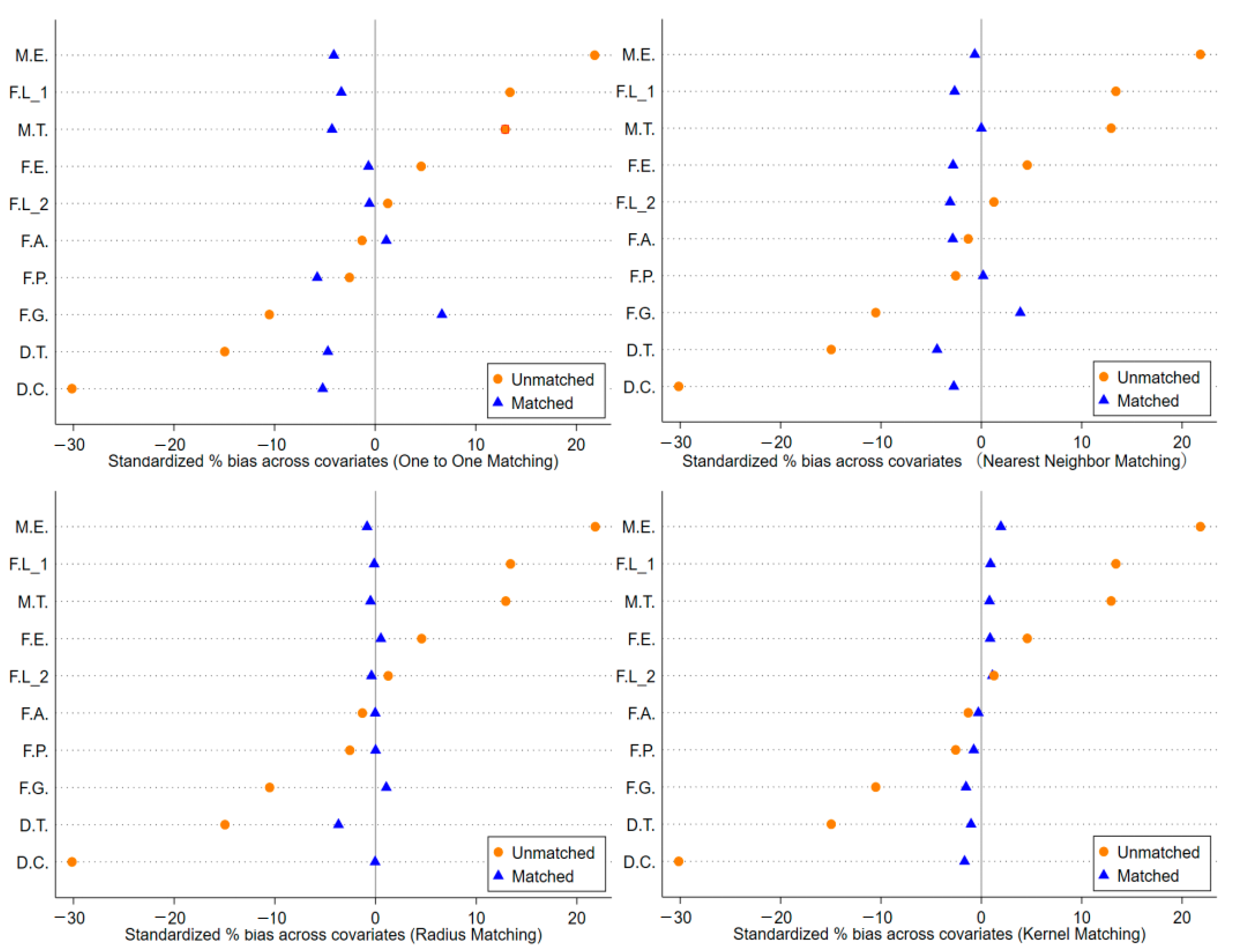
Figure 5 more intuitively depicts the standardized bias graphs under different matching methods both before matching and after matching. In the first place, according to the change characteristics of the results obtained before matching and after matching, the standardized bias distribution of each variable is scattered, and the deviation is relatively large before matching. However, after matching, the standardized bias of each variable was significantly narrowed overall. In the second place, from the matching results of different matching methods, it can be quite clearly seen that, in contrast to one-to-one matching, the standard bias of each variable after nearest neighbor matching, radius matching, and kernel matching all decrease substantially. In particular, the distribution of the standard bias of each variable after kernel matching is relatively more concentrated.
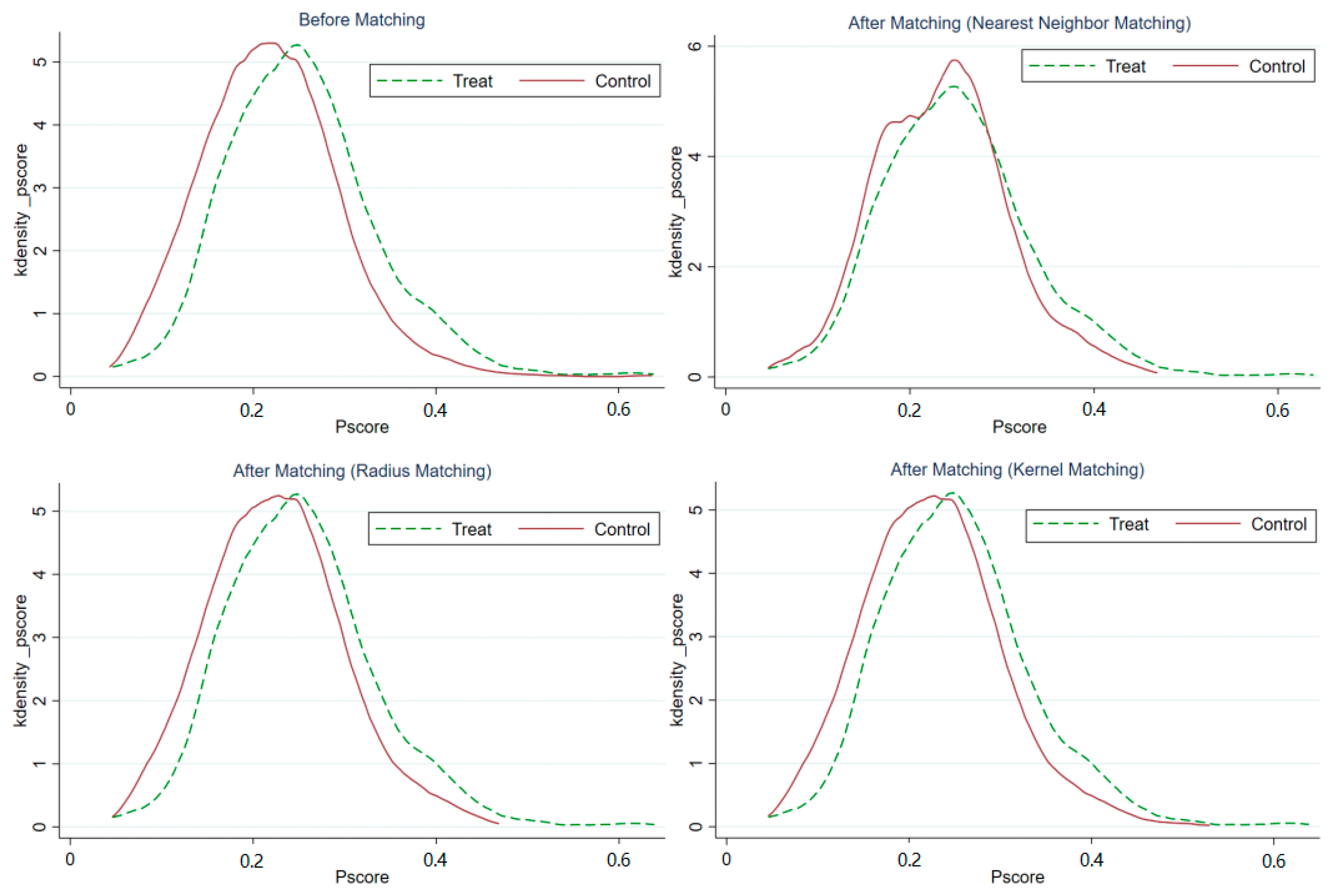
The kernel density estimate function distribution of the propensity matching score to before matching and after matching are depicted vividly in Figure 6. A comparison of the kernel density estimate function distribution for the four groups shows that, compared with the density estimate function distribution before matching, the treatment group after nearest neighbor matching, radius matching, and kernel matching has propensity scores relatively closer to the control group, which this means that one is able to find the matching sample to the treatment group from among the control group samples. In other words, we can distinguish between the matching samples for the family farms samples from an area with a demonstration farm and the family farms samples from an area that had not obtained a demonstration farm. At the same time, it also shows that the effect obtained from the sample data after matching can meet the common support hypothesis of PSM and that the matching effect of propensity score is better.

5.5. Sensitivity Analysis

Given that basis of the PSM approach is to control the effects of the measurable variables, it still introduces a “hidden bias” if there is selection on unobservable variables [54]. In order to avoid the impact caused by “hidden bias”, the level of bias should be estimated through sensitivity analysis [55,58], which aims to observe the sensitivity of PSM estimation results to “hidden bias.” The fundamental task of sensitivity analysis is to derive a range of gamma attributable to “hidden bias”. Gamma measures the departure degree from a study without “hidden bias” [59]. In view of this, this paper further examines the sensitivity of PSM estimation results to “hidden bias” based on the Rosenbaum bounds sensitivity analysis approach proposed by Rosenbaum et al. [55,58]. The sensitivity analysis of the Rosenbaum bounds is summarized neatly in Table 7. Among the terms used, “gamma” stands for the log odds of the differential assignment due to unobserved factors, “sig+” represents the upper-bound significance level, and “sig−” denotes lower-bound significance level. It should be illustrated, due to limited space, the Gamma values take values from 1 and increase by 0.2 increments until gamma = 3. The sensitivity analysis results fully reveal that the lower bound significance level of gamma at different value intervals was all less than 0.01, and that the upper bound significance level of gamma at different value intervals was also less than 0.01, as estimated by the three matching methods, including nearest neighbor matching, radius matching, and kernel matching. Therefore, in this paper, it is reasonable to believe that there is a close association between the demonstration farm and labor productivity, the estimation results obtained in this paper via the PSM method have good robustness, and the conclusions of the research are reliable and credible.

5.6. Discussions

Table 8 centrally reports the average treat effect on the treated of matched sample. Obtained by synthetically comparing the analysis data, the result of sample estimation before matching was determined to be 29.3543, which is completely consistent with the results of the single regression shown in Table 4, namely, the results of model (a) and model (b). After taking the nearest neighbor matching, the estimated value of ATT is 28.5108, and its corresponding t value is 8.4900, which is above the critical value of 2.58. This indicates that the estimated result of the matched sample passed the 1% significance level test, implying that, in the case of controlling for other covariates, the demonstration farm can significantly improve farm income by CNY285108 on average in the matched sample. After taking the radius matching method, the estimated value of ATT is 28.8509, and its corresponding t value is 9.0300, which indicates that the estimated result of the matched sample passes the 1% significance level test. This means that, when controlling for other covariates, the demonstration farm can significantly increase farm income by CNY288509 on average in the matched sample. After using the kernel matching, the estimated value of ATT is 29.1076, and its corresponding t value is 9.1700, indicating that the estimated result of the matched sample passes the 1% significance level test. This means that when controlling for other covariates, the demonstration farm can significantly raise farm income by CNY291077 on average in the matched sample.

6. Conclusions and Implications

In this paper, based on a sample of 1823 family farms in the mountainous areas of western China, the causal relationship of demonstration farm on labor productivity was empirically tested. Additionally, the PSM-logit model and sensitivity analysis wwere used. The conclusions of this paper are as follows.
Firstly, as the average agricultural labor productivity of the demonstration farm is CNY454898, which is 2.8 times higher than that of the non-demonstration farm, hypothesis 1 has been verified. Secondly, there is a significant positive correlation between demonstration family farm and agricultural labor productivity. Compared to family farms that did not obtain the demonstration farm, the use of demonstration farms in the case of adding all control variables, which can promote farm income by CNY301458 on average, gave significant values at the level of 1‰, verifying hypothesis 2. Thirdly, in the matched sample, and under scenarios controlling for other covariates, the use of demonstration farms, was shown to significantly enhance farm income of CNY285108, CNY288509, and CNY291077 on average, respectively. After taking the radius matching, the kernel matching, and the nearest neighbor matching, the average treat effect on the treated of matched sample passed the 1% significance level test. When propensity score matching is performed, most of the observed values are within the common support by the propensity score, indicating that the matching results have passed the balance test. Meanwhile, the sensitivity analysis results fully reveal that there is a close association between the demonstration farm and labor productivity, and the estimation results obtained in this paper by PSM method has good robustness, and the conclusions of the research are reliable and credible, meaning that hypothesis 3 has been verified. However, objectively speaking, the above research results may only be applicable to the mountainous area of western China and may not necessarily apply to the eastern or central regions of China, which may be greatly related to the varying degrees of differences in agricultural resource endowment, agricultural industry structure, agricultural industry resilience, and agricultural development potential in different regions of China.
Based on the above findings, the policy implications of this research are significant. First of all, farmers should actively develop family farms according to local conditions, and vigorously cultivate and develop demonstration farms [6,7,9,35,36,37], innovate experimental and demonstration models from the perspective of regional coordinated development [60], step up, publicize and promote unceasingly the typical cases and experience of demonstration farm, so as to encourage family farms to continuously improve labor productivity. Secondly, authorities should encourage family farms that have not been obtained demonstration farm to continue to give play to their comparative advantages, aggregate the optimized allocation and agglomeration effect of various resources, strengthen the professional skills education and management ability of farm owners, improve the quality and competitiveness of farm products, carry out continuous moderate scale management, summarize and promote the typical experience of the farm. Thirdly, on the basis of fully considering the factors of family farms, such as industrial foundation, development type, land continuity, convenient transportation, etc., authorities should innovate the management modes of mountainous planting or breeding and explore industrial models of mountain stereo agriculture, actions which in turn contribute to improving the labor productivity of family farms.
In addition, based on policy implications, this paper proposes the following future direction. The local government and its agricultural and rural departments should further improve the top-level design and supporting policies for high-quality development of family farms, optimizing and improving the developmental planning and construction system of family farms according to local conditions, strengthening the demonstrative establishment of family farms, accelerating the linkage and integration of family farms with other new type agricultural business entities, advancing high-quality development of agricultural modernization [61], and promoting sustainable development of agricultural and rural [62].

Author Contributions

T.H. and J.H. conceived and designed the research question. T.H. constructed the models and wrote the paper. J.H. and Q.H. reviewed and edited the manuscript. All authors have read and agreed to the published version of the manuscript.

Funding

This research was funded by the Chongqing Social Science Planning Project (grant no.: 2022BS051); the National Social Science Foundation of China (grant no.: 22BJY037), and the Chongqing Social Science Planning Chongqing Talent Scheme “Lump Sum System” Project (grant no.: 2022YC062).

Institutional Review Board Statement

Not applicable.

Informed Consent Statement

Not applicable.

Data Availability Statement

The data that support the finding of this study are available from the corresponding author upon reasonable request.

Acknowledgments

The authors are grateful to the anonymous referees who provided valuable comments and suggestions to significantly improve the quality of the paper. We gratefully acknowledge the Chongqing Social Science Planning Project (grant no.: 2022BS051); the National Social Science Foundation of China (grant no.: 22BJY037), and the Chongqing Social Science Planning Chongqing Talent Scheme “Lump Sum System” Project (grant no.: 2022YC062).

Conflicts of Interest

The authors declare no conflict of interest. There is no professional or other personal interest of any nature or kind in any product, service and/or company that could be construed as influencing the position presented in, or the review of, the manuscript entitled.

References

  1. Schultz, T.W. Transforming Traditional Agriculture; Liang, X.M., Ed.; The Commercial Press: Beijing, China, 2021; p. 175. ISBN 978-7-100-19459-4. [Google Scholar]
  2. D.E.E. Group. Economics of Development; Higher Education Press: Beijing, China, 2019; p. 438. ISBN 978-7-04-052212-9. [Google Scholar]
  3. Guth, M.; Stępień, S.; Smędzik-Ambroży, K.; Matuszczak, A. Is small beautiful? Techinical efficiency and environmental sustainability of small-scale family farms under the conditions of agricultural policy support. J. Rural. Stud. 2022, 89, 235–247. [Google Scholar] [CrossRef]
  4. Huang, T.; Xiong, B. Space Comparison of Agricultural Green Growth in Agricultural Modernization: Scale and Quality. Agriculture 2022, 12, 1067. [Google Scholar] [CrossRef]
  5. Huang, T.; Jiang, L. Nurturing the Family Farm to Help Get Rid of Poverty. Guizhou Daily, 23 October 2019. [Google Scholar] [CrossRef]
  6. Huang, T.; Yang, J. Analysis and evaluation of Social Benefits of Family Farm under the Rural Revitalization Strategy—Based on empirical test of 1,811 municipal Family Farms. J. Anshun Univ. 2020, 22, 34–37. [Google Scholar]
  7. Huang, T. Empirical study of Family Farm economic growth is based on Solow Growth Model—Data Verification from Tongren city. Jiangsu Agric. Sci. 2020, 48, 15–20. [Google Scholar]
  8. Guo, X.; Wu, F. Can Participation in Cooperatives Improve the Production Technical Efficiency of Family Farms? Soc. Sci. Front. 2022, 01, 66–79. [Google Scholar]
  9. Cai, R.; Wang, Z.; Du, Z. Are Model Family Farms More Technically Efficient? An Analysis Based on the Monitoring Data of National Family Farms. Chin. Rural. Econ. 2019, 3, 65–81. [Google Scholar]
  10. Zhao, C.; Kong, X.; Chou, H. Does the Expansion of Farm Size Contribute to the Reduction of Chemical Fertilizers?—Empirical Analysis Based on 1274 Family Farms in China. J. Agrotech. Econ. 2021, 4, 110–121. [Google Scholar]
  11. Wang, X.; Du, Z. Are Family Farms More Efficient?—A Comparative Study Based on Theory and Empirical Analysis. Dongyue Trib. 2020, 41, 172–181. [Google Scholar]
  12. The Central Committee Of China. Compilation of No.1 Documents of the CPC Central Committee and the State Council on the Work of “Agriculture, Rural and Farmers” (1982–2014); People’s Publishing House: Beijing, China, 2014. [Google Scholar]
  13. Some opinions of the CPC Central Committee and the State Council on strengthening reform and innovation efforts and accelerating agricultural modernization construction. Bull. State Counc. People’s Repub. China 2015, 5, 6–14.
  14. Some opinions of the CPC Central Committee and the State Council on implementing the new concept of development, accelerating agricultural modernization and achieving the goal of building a moderately prosperous society in all respects. Bull. State Counc. People’s Repub. China 2016, 6, 7–17.
  15. Some Opinions of the CPC Central Committee and the State Council on deepening the supply side structural reform of agriculture and accelerating the cultivation of new drivers of agricultural and rural development. Bull. State Counc. People’s Repub. China 2017, 2, 4–11.
  16. Opinions of the CPC Central Committee and the State Council on implementing the Rural Revitalization Strategy. Bull. State Counc. People’s Repub. China 2018, 5, 4–16.
  17. Some opinions of the CPC Central Committee and the State Council on adhering to the priority development of agriculture and rural areas and doing a good job in the work of “Agriculture, Rural and Farmers. Bull. State Counc. People’s Repub. China 2019, 7, 25–33.
  18. Opinions of the CPC Central Committee and the State Council on grasping the key work in the field of “Agriculture, Rural and Farmers” to ensure the realization of a moderately prosperous society in all respects on schedule. Bull. State Counc. People’s Repub. China 2020, 5, 6–12.
  19. Opinions of the CPC Central Committee and the State Council on comprehensively promoting rural revitalization and accelerating agricultural and rural modernization. Bull. State Counc. People’s Repub. China 2021, 7, 14–21.
  20. Opinions of the CPC Central Committee and the State Council on doing a good job in the key work of comprehensively promoting rural revitalization in 2022. Bull. State Counc. People’s Repub. China 2022, 7, 5–13.
  21. Guidance Opinions of the State Council on Promoting the Revitalization of Rural Industries. Bull. State Counc. People’s Repub. China 2019, 19, 21–26.
  22. Breitenbach, R.; Foguesatto, C.R. Should I stay or should I go? Gender differences and factors influencing family farm business succession in Rio Grande do Sul, Brazil. Land Use Policy 2023, 128, 106597. [Google Scholar] [CrossRef]
  23. de Souza, S.R.G.; Vale, D.; Nascimento, H.I.F.D.; Nagy, J.C.; Junior, A.H.M.D.S.; Rolim, P.M.; Seabra, L.M.J. Food Purchase from Family Farming in Public Institutions in the Northeast of Brazil: A Tool to Reach Sustainable Development Goals. Sustainability 2023, 15, 2220. [Google Scholar] [CrossRef]
  24. Van Balen, D.; Cuperus, F.; Haagsma, W.; De Haan, J.; Van Den Berg, W.; Sukkel, W. Crop yield response to long-term reduced tillage in a conventional and organic farming system on a sandy loam soil. Soil Till Res. 2023, 225, 105553. [Google Scholar] [CrossRef]
  25. Xiao, W.; Du, Z. Dutch Sample of Family Farm Development: Operational Characteristics and Institutional Practice. Chin. Rural. Econ. 2015, 2, 83–96. [Google Scholar]
  26. Becot, F.A.; Inwood, S.M. The case for integrating household social needs and social policy into the international family farm research agenda. J. Rural. Stud. 2020, 77, 185–198. [Google Scholar] [CrossRef]
  27. Zhu, X. French Family Farm Development Experience and Its Enlightenment to China. Rural. Econ. 2013, 11, 122–126. [Google Scholar]
  28. Yagi, H.; Hayashi, T. Machinery utilization and management organization in Japanese rice farms: Comparison of single-family, multifamily, and community farms. Agribusiness 2021, 37, 393–408. [Google Scholar] [CrossRef]
  29. Lang, X. Family Farms: Experience and Inspiration Illustrated with Examples of France and Japan. Stud. Mao Zedong Deng Xiaoping Theor. 2013, 10, 36–41. [Google Scholar]
  30. Qian, Z.; Li, Y. The Values and Influence Factors of Family Farms’ Efficiency—Empirical Study Based on 2017 Data of 943 Family Farms in Songjiang, Shanghai. J. Manag. World 2020, 36, 168–181. [Google Scholar]
  31. Guo, X.; Leng, C. Research on the Ten Characteristics of Family Farm Development in China—Based on the comparative analysis of 607 family farms in Wuhan and Langxi. Econ. Rev. J. 2018, 10, 43–58. [Google Scholar]
  32. Chen, N.; Hao, Q. Empirical study on the environmental elements of family farm’s development: Based on the survey data from Yanbian of Jilin Province. Res. Agric. Mod. 2017, 38, 429–436. [Google Scholar]
  33. Chen, D. Research on Family Farm Cultivation Problem—Based on Research and Analysis of Langxi Family Farm in Anhui Province. Theory Reform 2015, 5, 87–91. [Google Scholar]
  34. Lu, H.; Zhu, Y. Research on Development Model of Family Farm Based on Scale Questionnaire Analysis—Taking Ningbo City, Zhejiang Province as an Example. Issues Agric. Econ. 2015, 36, 19–26. [Google Scholar]
  35. Huang, T.; Huang, Q.; Hu, J. The influence of pilot identification on the economic benefit of Family Farm—Empirical Test based on PSM Method and Multiple Logit Model. World Agric. 2020, 9, 56–64. [Google Scholar]
  36. Huang, T. Sustainable development of Family Farms of Rural Revitalization Strategy: Practical review of Ecological Benefits. J. Adm. Manag. Inst. Minist. Agric. Rural. Aff. 2020, 3, 42–46. [Google Scholar]
  37. Huang, T.; Hu, J. Economic Benefit Analysis and Prospect of Family Farm under the Rural Revitalization Strategy. Agric. Outlook 2020, 16, 26–31. [Google Scholar]
  38. Guan, F. The Land Scale of Grain Production Family Farms in North China Plain: An Example from Henan, a Major Grain Production Province. Chin. Rural. Econ. 2018, 10, 22–38. [Google Scholar]
  39. Wang, X.; Du, Z. Small Farmers and Family Farms: Connotation Characteristics, Attribute Differences and Evolution Logic. Theory J. 2020, 5, 93–101. [Google Scholar]
  40. Kusz, B.; Kusz, D.; Bąk, I.; Oesterreich, M.; Wicki, L.; Zimon, G. Selected Economic Determinants of Labor Profitability in Family Farms in Poland in Relation to Economic Size. Sustainability 2022, 14, 13819. [Google Scholar] [CrossRef]
  41. Lairez, J.; Affholder, F.; Scopel, E.; Leudpanhane, B.; Wery, J. Sustainability assessment of cropping systems: A field-based approach on family farms. Application to maize cultivation in Southeast Asia. Eur. J. Agron. 2023, 143, 126716. [Google Scholar] [CrossRef]
  42. Aubron, C.; Bainville, S.; Philippon, O.; Dorin, B. Neither Corporate, Nor Family: The Indian “Patronal” Farm. Front. Sustain. Food Syst. 2022, 6, 850545. [Google Scholar] [CrossRef]
  43. Smędzik-Ambroży, K.; Guth, M.; Majchrzak, A.; Muntean, A.C.; Maican, S. The Socio-Economics Factors in Family Farms with Different Economic Sustainability Levels from Central and Eastern Europe. Sustainability 2021, 13, 8262. [Google Scholar] [CrossRef]
  44. Zhao, H.; Liu, F. Analysis on the Dilemma of Family Farm in American Capitalist System. China Rev. Political Econ. 2020, 11, 146–183. [Google Scholar]
  45. Wu, J.; Han, D.; Ruan, R. Agriculture Informatization and Quality of Agricultural Products: Analysis on the Behavior of Quality Certification of Agricultural Products Based on Family Farms. J. Nanjing Agric. Univ. 2022, 22, 172–184. [Google Scholar]
  46. Yao, L.; Ma, Y. Foreign Family Farm Financial Service Legal System and Its Enlightenment to China. Theory Pract. Financ. Econ. 2021, 42, 152–160. [Google Scholar]
  47. Moreno Ramos, R.N. Family labour organization for dairy farming in western Mexico. Between the search for productivity and wellbeing. J. Rural. Stud. 2021, 88, 354–367. [Google Scholar] [CrossRef]
  48. Guo, X.; Gong, G. Can Adoption of New Technologies Raise Economic Efficiency of Family Farms?—From the Perspective of Realization of New Technological Demand. J. Huazhong Agric. Univ. 2021, 1, 33–42. [Google Scholar]
  49. Yi, C.; Duan, H. Bottlenecks and Realization Paths of Starting a Business on Family Farm—Based on Field Investigation in Eight Areas of Hunan Province. Issues Agric. Econ. 2020, 2, 126–134. [Google Scholar]
  50. Hu, J.; Zhang, X.; Wang, T. Spatial Spillover Effects of Resource Misallocation on the Green Total Factor Productivity in Chinese Agriculture. Int. J. Environ. Res. Public Health 2022, 19, 15718. [Google Scholar] [CrossRef]
  51. Huang, T.; Xiong, B. Looking Back and Looking Forward: On the Modernization of Agriculture and Rural Areas from the Spirit of the Central Rural Work Conference in the New Era’s Decade. Leadersh. Sci. 2022, 11, 126–129. [Google Scholar]
  52. Guiding Opinions on Implementing the Family Farm Cultivation Plan. Bull. Minist. Agric. Rural. Aff. People’s Repub. China 2019, 9, 36–39.
  53. Rubin Donald, B. Estimating causal effects of treatments in randomized and nonrandomized studies. J. Educ. Psychol. 1974, 66, 688–701. [Google Scholar] [CrossRef] [Green Version]
  54. Chen, Q. Advanced Econometrics and Stata Applications; Higher Education Press: Beijing, China, 2014. [Google Scholar]
  55. Guo, S.; Fraser, M.W. Propensity Score Analysis: Statistical Methods and Applications; Chongqing University Press: Chongqing, China, 2012. [Google Scholar]
  56. Rosenbaum, P.R.; Rubin Donald, B. Constructing a Control Group Using Multivariate Matched Sampling Methods That Incorporate the Propensity Score. Am. Stat. 1985, 39, 33–38. [Google Scholar]
  57. Huang, T.; Lu, D.; Yang, J. Comprehensive Evaluation and Spatio-temporal Variation Analysis of Cutivated Land in Provincial Area Based on GIS—A Case Study in Guizhou Province. Res. Soil Water Conserv. 2017, 24, 253–257. [Google Scholar]
  58. Rosenbaum, P.R.; Rubin Donald, B. The Central Role of the Propensity Score in Observational Studies for Causal Effects. Biometrika 1983, 70, 41–55. [Google Scholar] [CrossRef]
  59. Rosenbaum, P.R. Observational Studies; Springer: Berlin/Heidelberg, Germany, 2002. [Google Scholar]
  60. Li, Q.; Hu, Y. Chinese style modernization from the perspective of regional coordinated development. J. Guizhou Prov. Party Sch. 2023, 1, 29–36. [Google Scholar]
  61. Huang, T.; Huang, Q.; Xu, D. Agricultural Modernization in Southwest Minority Mountain Areas from the Perspective of Common Prosperity: Theory, Policy and Practice. Chongqing Soc. Sci. 2023, 5, 30–46. [Google Scholar] [CrossRef]
  62. Huang, T.; Huang, Q. Research on Agricultural and Rural Public Governance and Sustainable Development: Evidence from 2350 Data. Sustainability 2023, 15, 7876. [Google Scholar] [CrossRef]
Figure 1. Theoretical mechanism for sustainable development between demonstration farm and agricultural labor productivity.
Sustainability 15 09560 g001
Figure 2. Common support of the propensity score.
Sustainability 15 09560 g002
Figure 3. General steps of the propensity score matching.
Sustainability 15 09560 g003
Figure 4. The common support of the Propensity Matching Score.
Sustainability 15 09560 g004
Figure 5. The standardized % bias across variables.
Sustainability 15 09560 g005
Figure 6. The kernel density function distribution of the propensity score to before matching and after matching.
Sustainability 15 09560 g006
Table 1. The settings and definitions of the variables.
Variables ClassificationVariable NameVariable SymbolVariable DefinitionsVariable Assignment
Dependent VariableLabor ProductivityL.P.The per capita production value of family farmCalculate according to the annual output value of family farm and the family laborers
Core Independent VariableDemonstration FarmD.F.Whether it is recognized as a demonstrative family farm1 = Family farm is a demonstration farm; 0 = Otherwise
Control VariableHead Farmer GenderF.G.The gender of the head farmer1 = Head farmer is male; 0 = Otherwise
Head Farmer AgeF.A.The age of the head farmerStatistics by actual age
Head Farmer EducationF.E.The educational level of the head farmer1 = Illiteracy; 2 = Primary school level; 3 = Junior high level; 4 = Senior high level or secondary vocational school level; 5 = College degree or above
Family LaborersF.L_1The number of family laborers engaging in agricultureStatistics by the numerical value
Farm ProductsF.P.The types of agricultural products operated by family farms1 = Single planting industry; 2 = Single breeding industry; 3 = Combination of planting and breeding; 4 = Mixed planting industry; 5 = Mixed breeding industry
Farm LandF.L_2The contiguous land area of family farmTake logarithm according to the numerical value
Managements TypesM.T.The managements types or models of family farm1 = Mountainous planting; 2 = Planting on dam land; 3 = Animal husbandry; 4 = Aquaculture; 5 = Integrated planting and breeding
Management ExperienceM.E.Operating years after being recognized as a family farmStatistics by the numerical value
Farm Distance_CountyD.C.The distance from the head farmer location to the countyStatistics by actual distance
Farm Distance_TownD.T.The distance from the head farmer location to the commercial market townStatistics by actual distance
Table 2. The descriptive statistics analysis of the variables.
StatisticControl GroupTreated Group
MeanSt. Dev.SkewnessKurtosisNMeanSt. Dev.SkewnessKurtosisN
L.P.16.135538.414017.7482404.3198141145.489860.28224.529531.2134412
F.G.0.85900.3482−2.06275.254614110.82040.3843−1.66933.7865412
F.A.42.24818.5314−0.44444.4944141142.13598.6332−0.48004.3414412
F.E.3.20690.7074−0.12544.177414113.24030.7500−0.14664.3000412
F.L_13.57341.80292.574817.814314113.88352.73066.746880.3920412
F.P.2.31041.26770.73602.318714112.27911.18060.83232.6750412
F.L_2178.7068167.915035.30371294.55001411171.3880505.979713.5441228.8064412
M.T.2.40681.14680.45332.711014112.55341.12030.32892.8296412
M.E.4.16651.4046−0.11763.489614114.46361.31660.59464.0862412
D.C.38.078925.35541.16314.0376141131.092120.76811.54406.6040412
D.T.9.489710.15934.004125.546214118.07698.67883.990225.3037412
Table 3. The correlation analysis of variables.
D.F.F.G.F.A.F.E.F.L_1F.P.F.L_2M.T.M.E.D.C.D.T.L.P.
D.F.1.0000
F.G.−0.0452 *1.0000
(0.0536)
F.A.−0.00550.03321.0000
(0.8150)(0.1562)
F.E.0.01950.0055−0.1474 ***1.0000
(0.4065)(0.8153)(0.0000)
F.L_10.0632 ***0.0222−0.01400.0389 *1.0000
(0.0069)(0.3431)(0.5490)(0.0966)
F.P.−0.0105−0.0335−0.0176−0.0255−0.00021.0000
(0.6545)(0.1529)(0.4529)(0.2764)(0.9940)
F.L_2−0.00210.0144−0.02340.00270.0221−0.02801.0000
(0.9278)(0.5380)(0.3175)(0.9098)(0.3459)(0.2327)
M.T.0.0537 **0.0324−0.0573 **−0.02010.01150.2347 ***−0.0503 **1.0000
(0.0219)(0.1661)(0.0143)(0.3908)(0.6249)(0.0000)(0.0317)
M.E.0.0894 ***−0.1186 ***−0.0892 ***−0.1345 ***0.02770.0126−0.03300.00371.0000
(0.0001)(0.0000)(0.0001)(0.0000)(0.2377)(0.5915)(0.1585)(0.8759)
D.C.−0.1190 ***0.0428 *0.03830.0414 *−0.0845 ***−0.01810.0519 **−0.0598 **0.03281.0000
(0.0000)(0.0675)(0.1018)(0.0769)(0.0003)(0.4402)(0.0266)(0.0107)(0.1620)
D.T.−0.0599 **0.0316−0.03080.0445 *−0.0183−0.0067−0.0140−0.0207−0.01510.1948 ***1.0000
(0.0105)(0.1773)(0.1887)(0.0573)(0.4345)(0.7734)(0.5497)(0.3767)(0.5187)(0.0000)
L.P.0.2672 ***−0.0386 *−0.0465 **0.0826 ***−0.1540 ***−0.0405 *−0.00280.03740.0026−0.00830.01521.0000
(0.0000)(0.0999)(0.0472)(0.0004)(0.0000)(0.0842)(0.9051)(0.1106)(0.9110)(0.7221)(0.5162)
Note: Significance in parentheses, * p < 0.10, ** p < 0.05, *** p < 0.01.
Table 4. Benchmark Regression Analysis of variables.
Model (a)Model (b)Model (c)Model (d)
D.F.29.3543 *** (2.4810)29.3543 *** (3.1392)30.1458 *** (2.4666)30.1458 *** (3.0579)
F.G. −3.6700 (2.8766)−3.6700 (3.1306)
F.A. −0.1842 (0.1212)−0.1842 * (0.0924)
F.E. 4.4703 ** (1.4589)4.4703 * (1.9720)
F.L_1 −4.0348 *** (0.5005)−4.0348 *** (0.7039)
F.P. −1.8423 * (0.8397)−1.8423 ** (0.5670)
F.L_2 1.7056 ** (0.5839)1.7056 *** (0.4835)
M.T. 2.5096 * (0.9861)2.5096 ** (0.9237)
M.E. −0.7010 (0.7571)−0.7010 (1.1305)
D.C. −0.0059 (0.0432)−0.0059 (0.0430)
D.T. 0.1071 (0.1052)0.1071 (0.1286)
_cons16.1355 *** (1.1794)16.1355 *** (1.0228)21.3053 * (9.8379)21.33053 ** (7.8371)
F-test139.9987.4421.8214.13
N1823182318231823
R20.07140.07140.11700.1170
Note: Standard errors in parentheses, * p < 0.05, ** p < 0.01, *** p < 0.001.
Table 5. The regression results of the PSM-Logit.
VariableCoefficientStd. Err.ZP > |Z|[95% Conf. Interval]
F.G.−0.20110.1543−1.30000.1930−0.50350.1013
F.A.0.00460.00690.68000.4990−0.00880.0181
F.E.0.12510.08041.56000.1200−0.03240.2826
F.L_10.0484 *0.02621.85000.0650−0.00300.0997
F.P.−0.05920.0485−1.22000.2220−0.15430.0359
F.L_20.03200.03220.99000.3200−0.03110.0951
M.T.0.1377 ***0.05362.57000.01000.03270.2427
M.E.0.1619 ***0.04303.76000.00000.07750.2462
D.C.−0.0126 ***0.0027−4.63000.0000−0.0179−0.0073
D.T.-0.01110.0070−1.59000.1120−0.02470.0026
_cons−2.3315 ***0.5507−4.23000.0000−3.4109−1.2522
Number of obs1823
LR chi2(10)61.96
Prob > chi20.0000
Pseudo R20.0318
Note: * p < 0.10, *** p < 0.01.
Table 6. The balance test of the matching results.
VariableMatching MethodTreatedControl%BiasT-Stat.Prob.
F.G.Unmatched0.82040.8590−10.5000−1.93000.0540 *
Nearest Neighbor Matching0.82200.80773.90000.52000.6000
Radius Matching0.82200.81801.10000.15000.8840
Kernel Matching0.82000.8256−1.5000−0.21000.8340
F.A.Unmatched42.136042.2480−1.3000−0.23000.8150
Nearest Neighbor Matching42.093042.3370−2.9000−0.41000.6800
Radius Matching42.093042.09500.00000.00000.9960
Kernel Matching42.097042.1230−0.3000−0.04000.9650
F.E.Unmatched3.24033.20694.60000.83000.4070
Nearest Neighbor Matching3.24393.2644−2.8000−0.40000.6920
Radius Matching3.24393.24010.50000.07000.9410
Kernel Matching3.24093.23450.90000.12000.9020
F.L_1Unmatched3.88353.573413.40002.70000.0070 ***
Nearest Neighbor Matching3.76103.8226−2.7000−0.46000.6470
Radius Matching3.76103.7641−0.1000−0.02000.9810
Kernel Matching3.79563.77460.90000.15000.8840
F.P.Unmatched2.27912.3104−2.6000−0.45000.6550
Nearest Neighbor Matching2.28052.27830.20000.03000.9790
Radius Matching2.28052.28040.00000.00001.0000
Kernel Matching2.28222.2915−0.8000−0.11000.9120
F.L_2Unmatched3.65433.62991.30000.23000.8210
Nearest Neighbor Matching3.64003.7003−3.1000−0.45000.6560
Radius Matching3.64003.6478−0.4000−0.06000.9540
Kernel Matching3.64863.62721.10000.16000.8750
M.T.Unmatched2.55342.406812.90002.29000.0220 **
Nearest Neighbor Matching2.55122.55120.00000.00001.0000
Radius Matching2.55122.5569−0.5000−0.07000.9440
Kernel Matching2.55722.54800.80000.11000.9100
M.E.Unmatched4.46364.166521.80003.83000.0000 ***
Nearest Neighbor Matching4.45854.4675−0.7000−0.09000.9260
Radius Matching4.45854.4700−0.8000−0.12000.9040
Kernel Matching4.46474.43821.90000.28000.7800
D.C.Unmatched31.092038.0790−30.1000−5.11000.0000 ***
Nearest Neighbor Matching31.116031.7510−2.7000−0.43000.6700
Radius Matching31.116031.12700.0000−0.01000.9940
Kernel Matching31.103031.4910−1.7000−0.27000.7910
D.T.Unmatched8.07699.4897−15.0000−2.56000.0100 ***
Nearest Neighbor Matching8.06348.4799−4.4000−0.66000.5070
Radius Matching8.06348.4111−3.7000−0.55000.5840
Kernel Matching8.08348.1803−1.0000−0.17000.8670
Note: * p < 0.10, ** p < 0.05, *** p < 0.01.
Table 7. The sensitivity analysis of the Rosenbaum bounds.
GammaNearest Neighbor MatchingRadius MatchingKernel Matching
sig+sig−sig+sig−sig+sig−
1.00.0000000.0000000.0000000.0000000.0000000.000000
1.20.0000000.0000000.0000000.0000000.0000000.000000
1.40.0000000.0000000.0000000.0000000.0000000.000000
1.60.0000000.0000000.0000000.0000000.0000000.000000
1.80.0000000.0000000.0000000.0000000.0000000.000000
2.00.0000000.0000000.0000000.0000000.0000000.000000
2.20.0000000.0000000.0000000.0000000.0000000.000000
2.40.0000000.0000000.0000000.0000000.0000000.000000
2.60.0000000.0000000.0000060.0000000.0000010.000000
2.80.0000050.0000000.0000540.0000000.0000110.000000
3.00.0000370.0000000.0003340.0000000.0000780.000000
Table 8. The average treat effect on the treated of matched sample.
SampleUnmatchedATT
Nearest Neighbor MatchingRadius MatchingKernel Matching
Treated45.489845.666845.666845.5895
Controls16.135517.156016.815916.4818
Difference29.354328.510828.850929.1077
Std. Err.2.48093.35923.19663.1744
T-Statistic11.83008.49009.03009.1700
Disclaimer/Publisher’s Note: The statements, opinions and data contained in all publications are solely those of the individual author(s) and contributor(s) and not of MDPI and/or the editor(s). MDPI and/or the editor(s) disclaim responsibility for any injury to people or property resulting from any ideas, methods, instructions or products referred to in the content.