
Characterization of the Coastal Vulnerability in Different Geological Settings: A Comparative Study on Kerala and Tamil Nadu Coasts Using FuzzyAHP

 , ,
, , 
 ,
, 
Abstract
1. Introduction
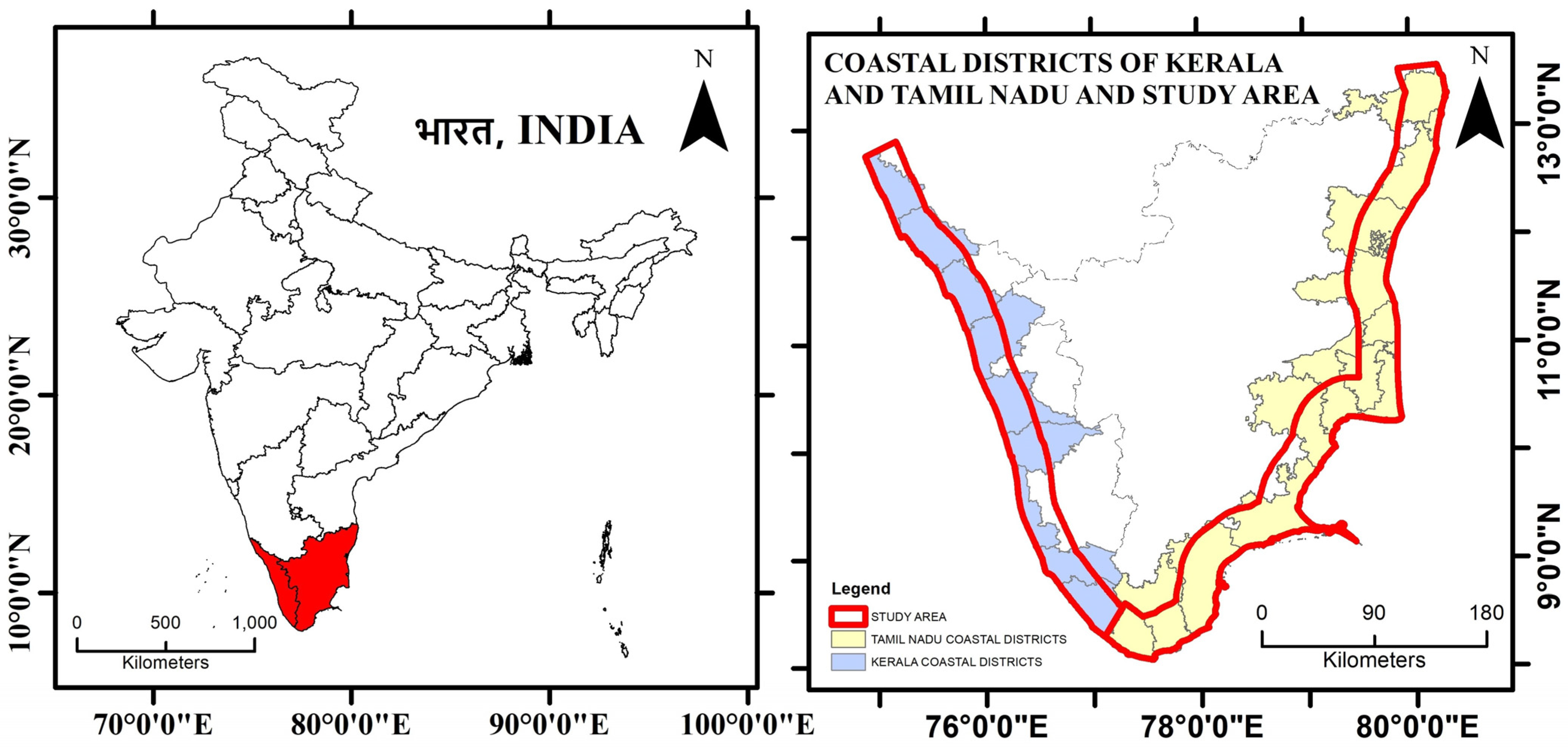
2. Study Area
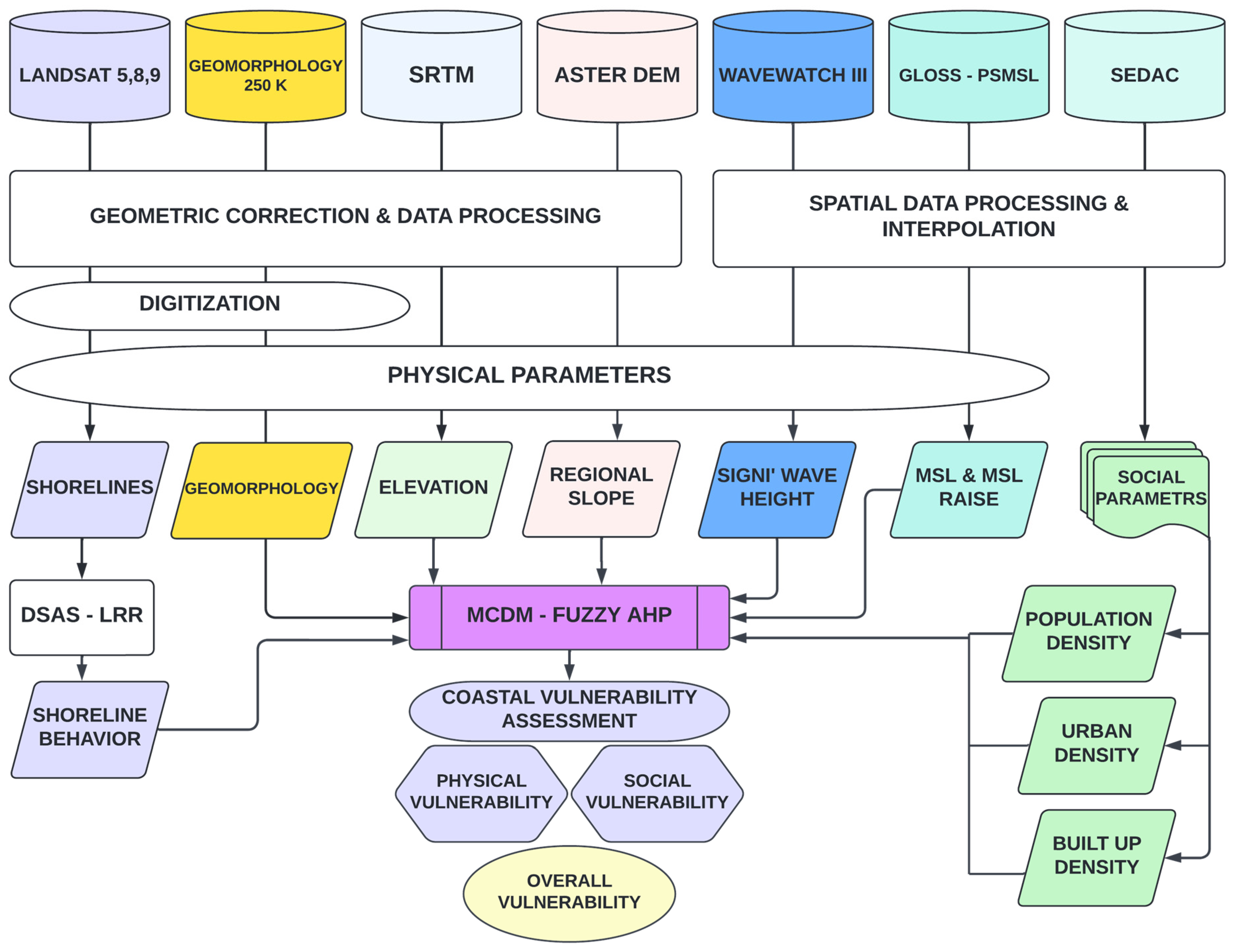
3. Materials and Methods
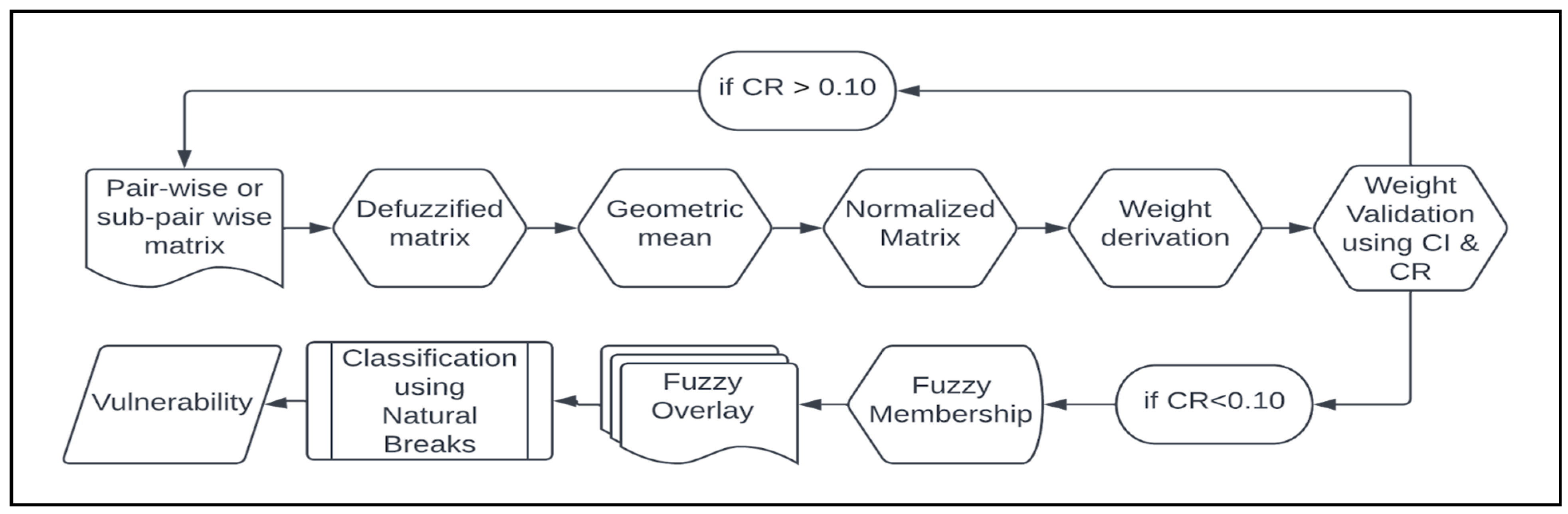
Coastal Vulnerability Assessment
4. Results
4.1. Hydro–Geographic Parameters
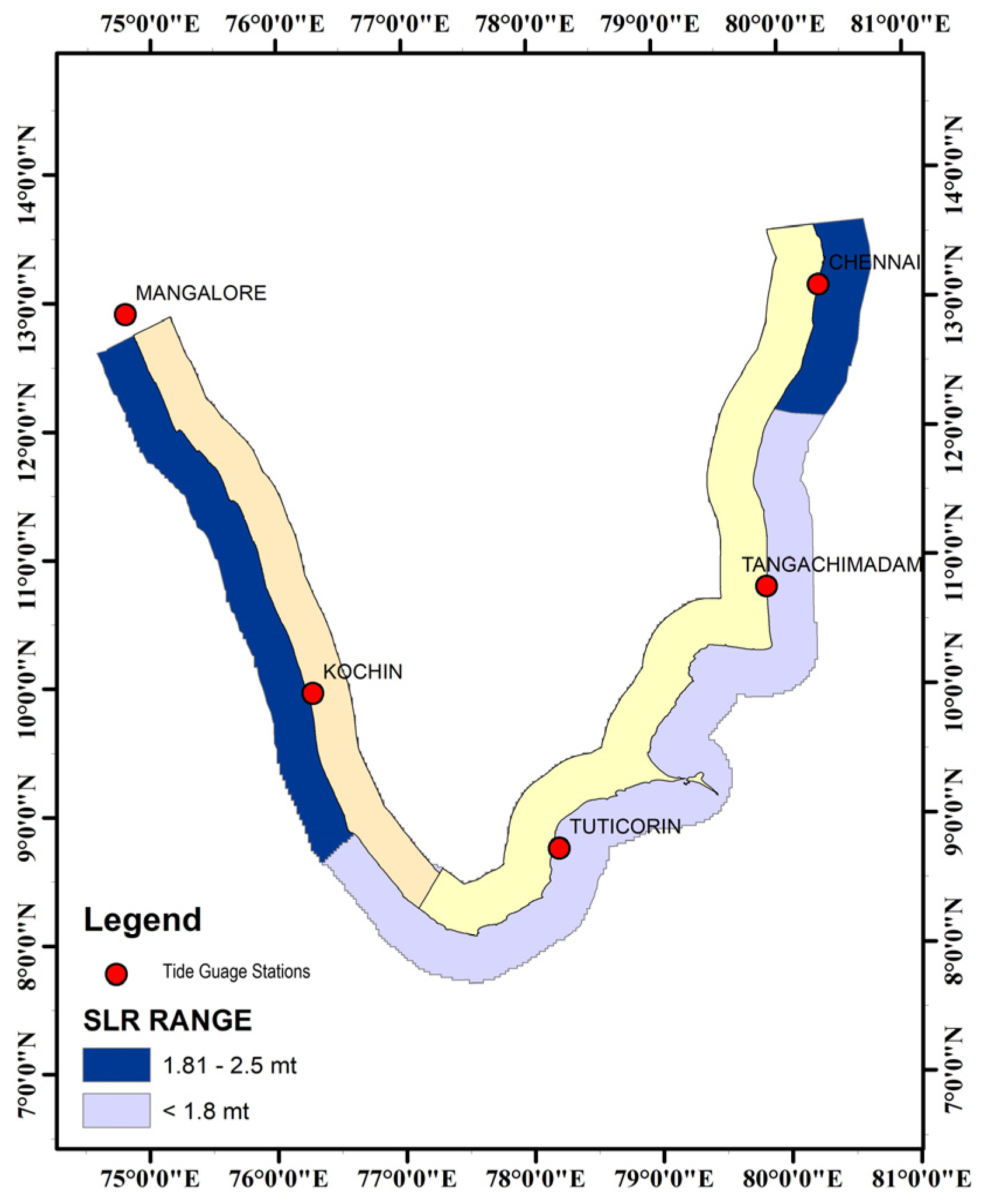
4.1.1. Mean Sea Level Rise
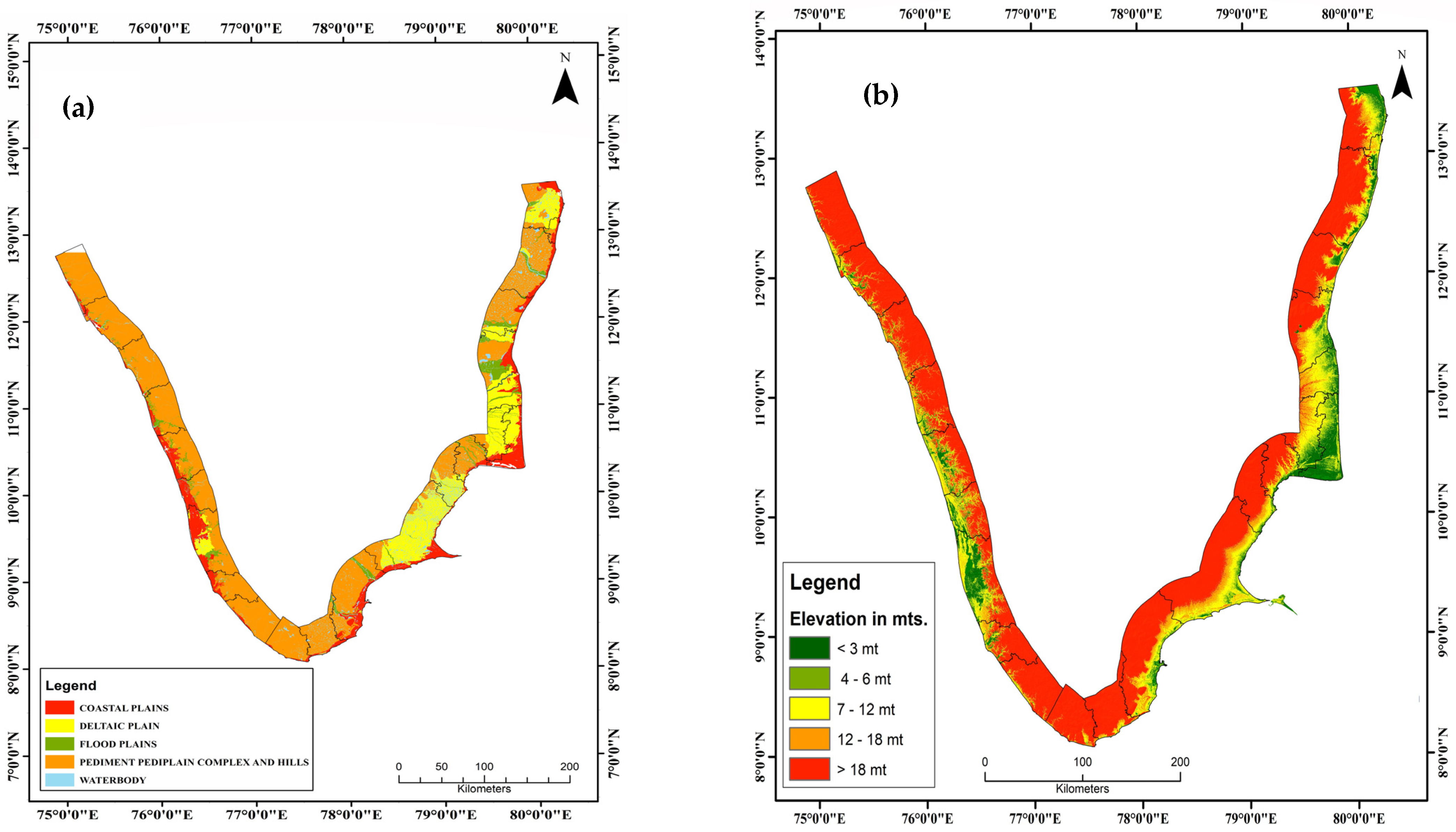
4.1.2. Geomorphology
4.1.3. Regional Elevation
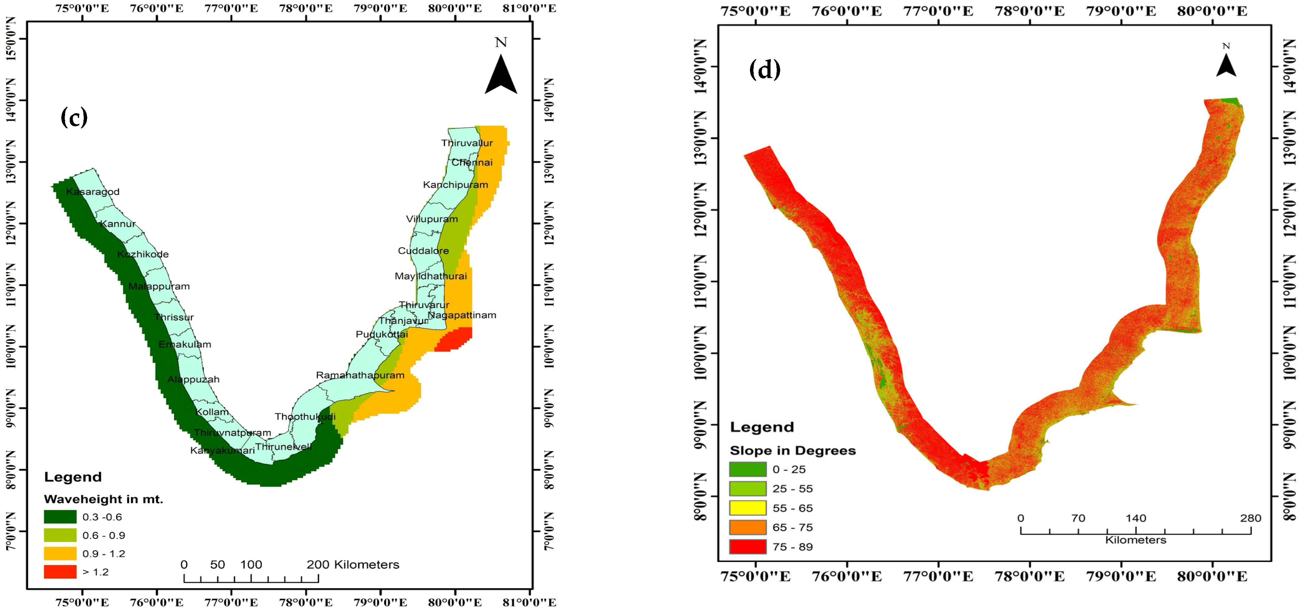
4.1.4. Surface Significant Wave Height
4.1.5. Regional Slope
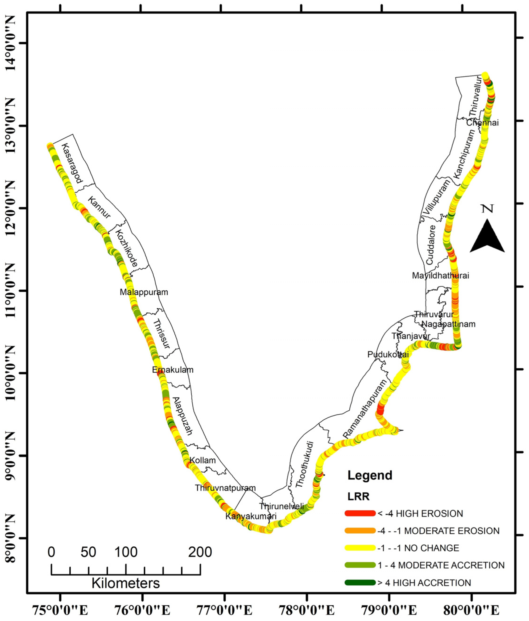
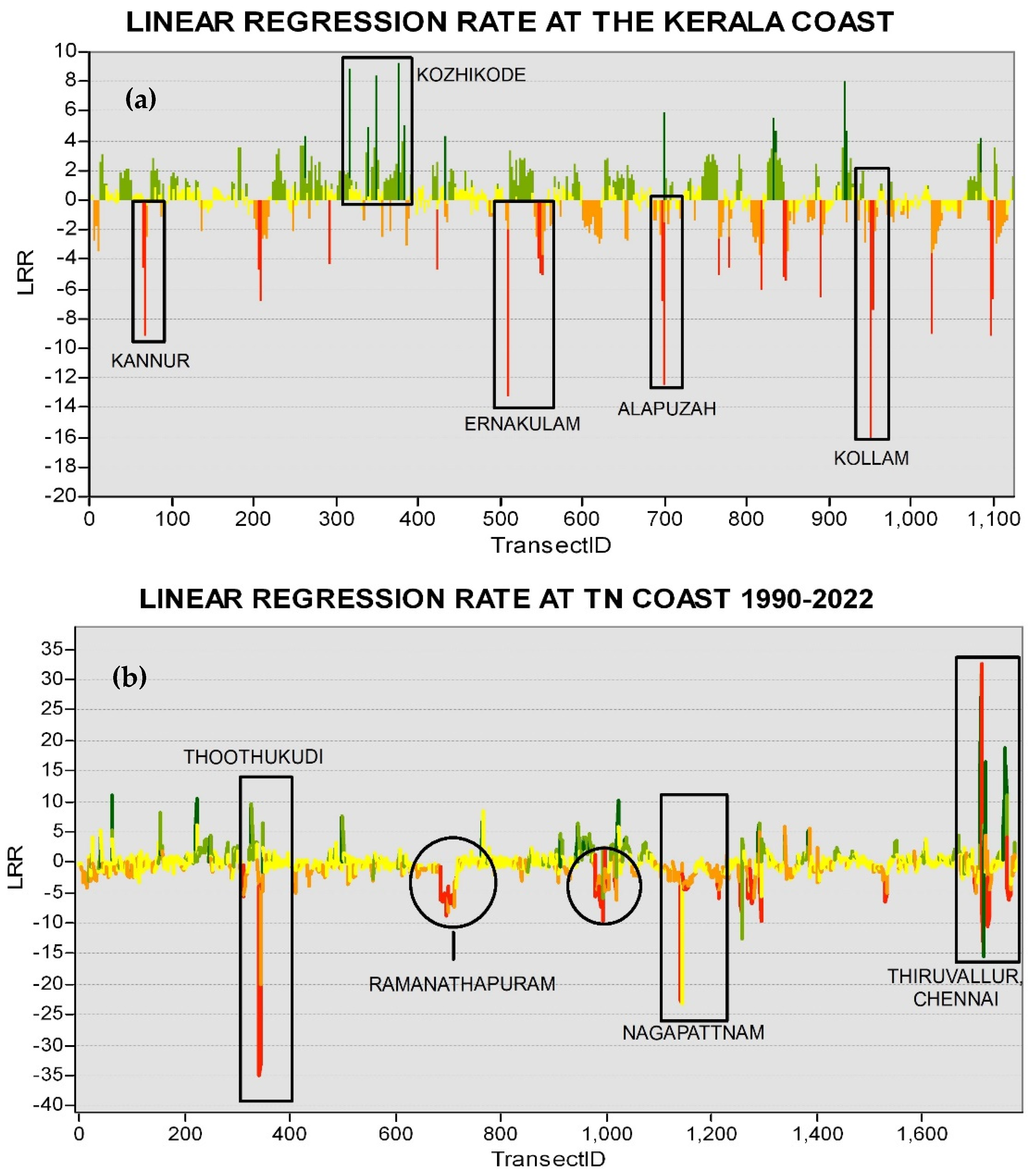
4.1.6. Shoreline Behavior using Linear Regression Rate
4.2. Socio-Economic Parameters
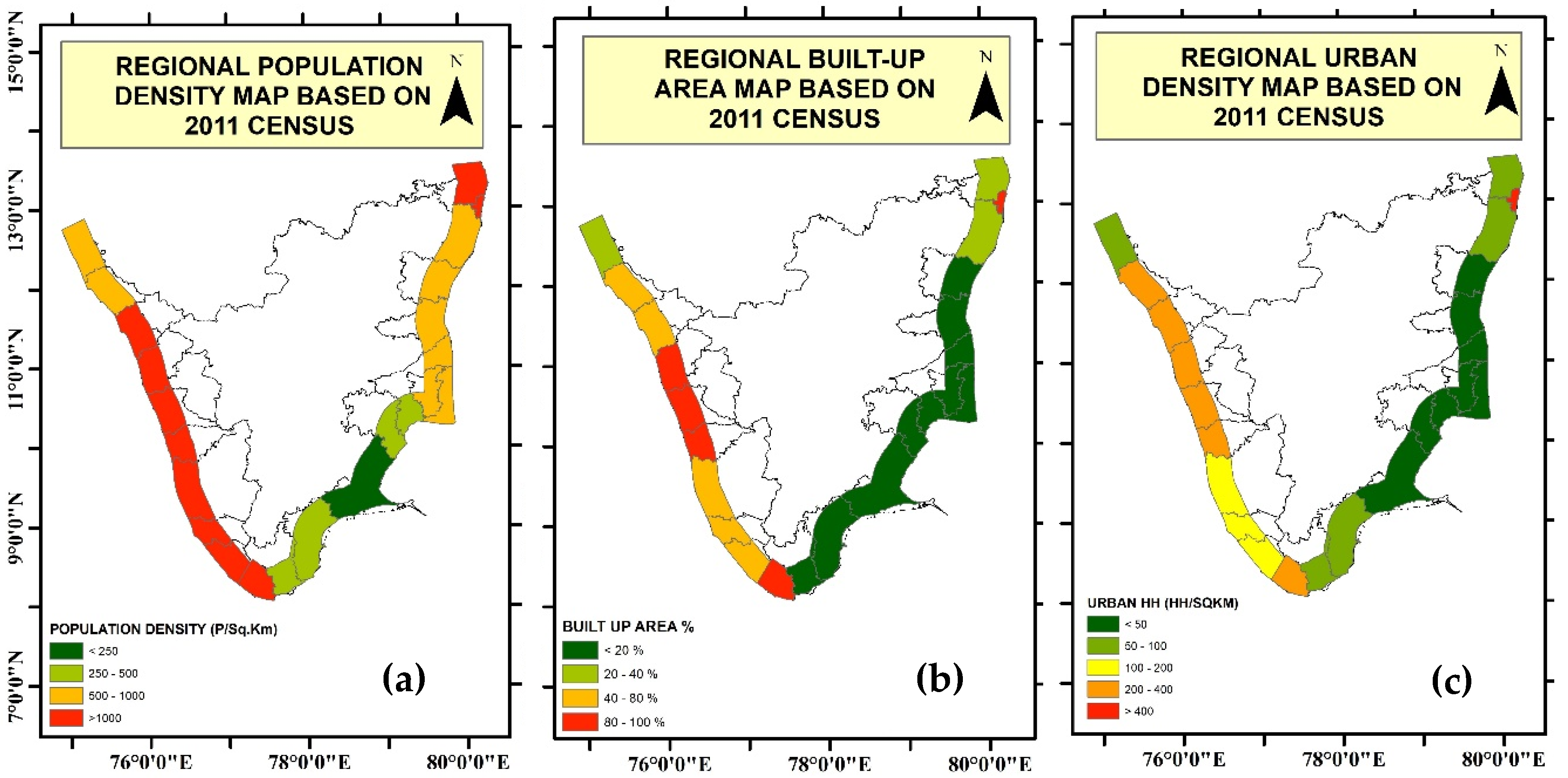
4.2.1. Regional Population Density
4.2.2. Regional Built-Up Area and Urban Density
4.3. Physical Vulnerability Assessment
4.4. Social Vulnerability Assessment
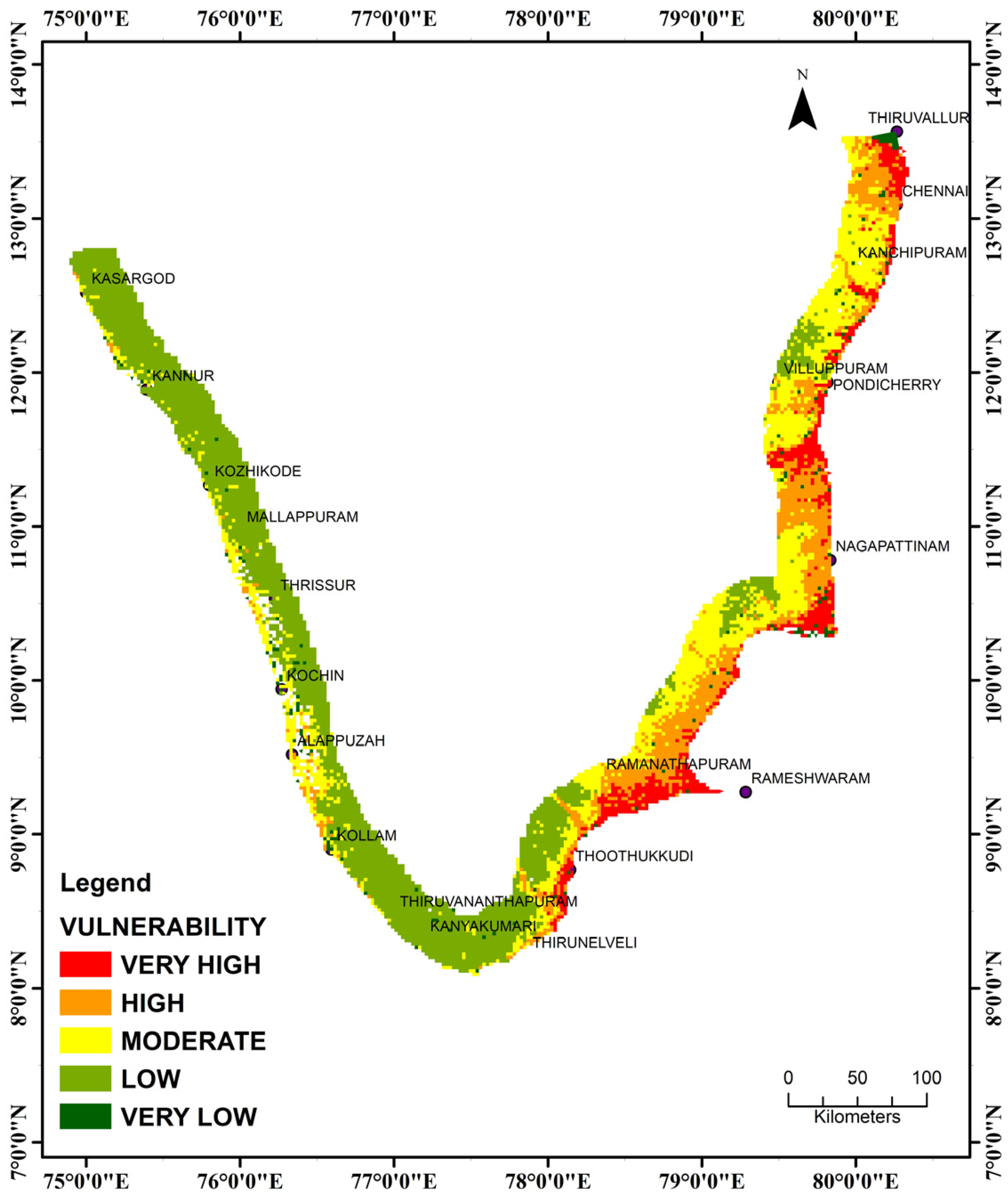
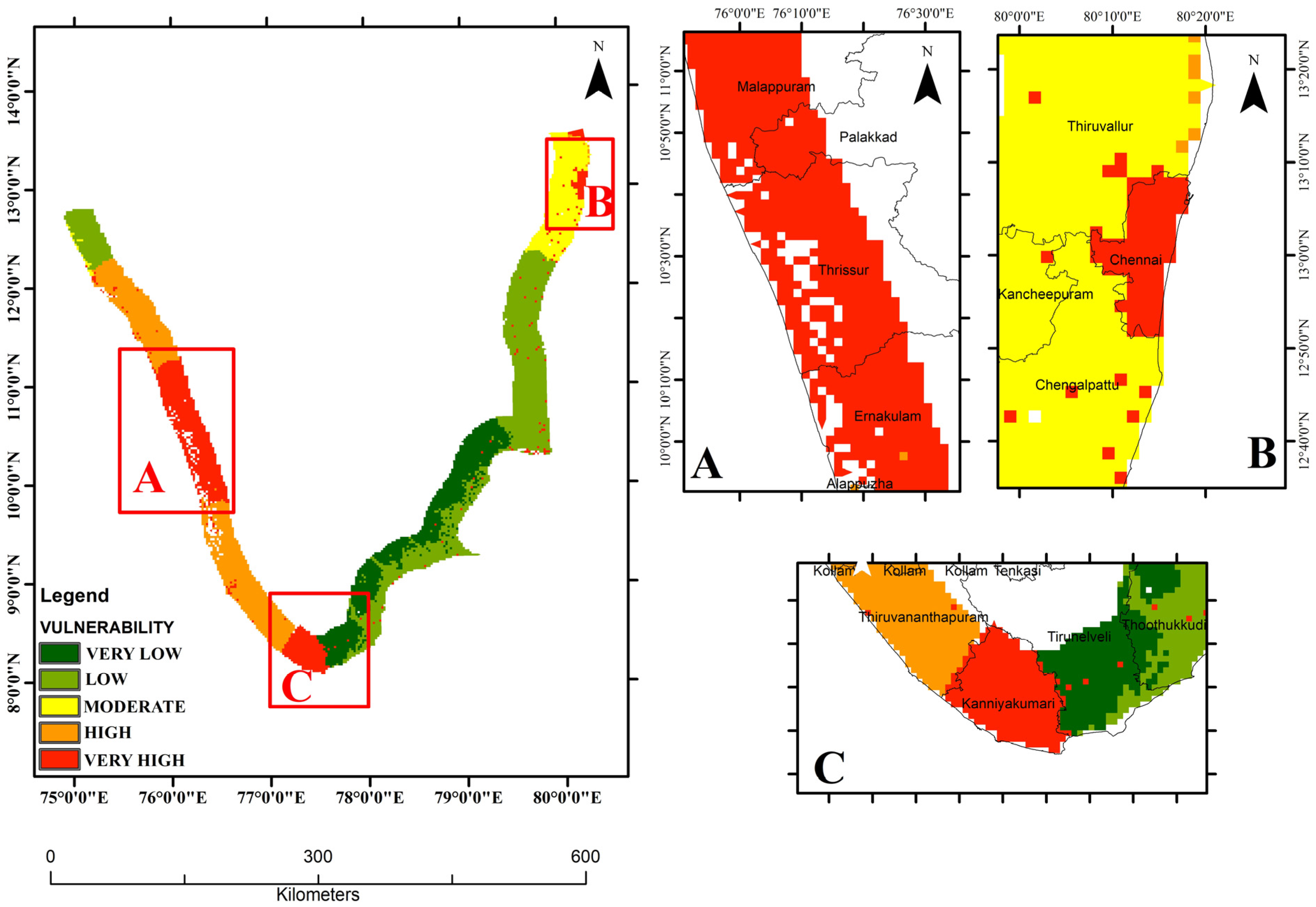
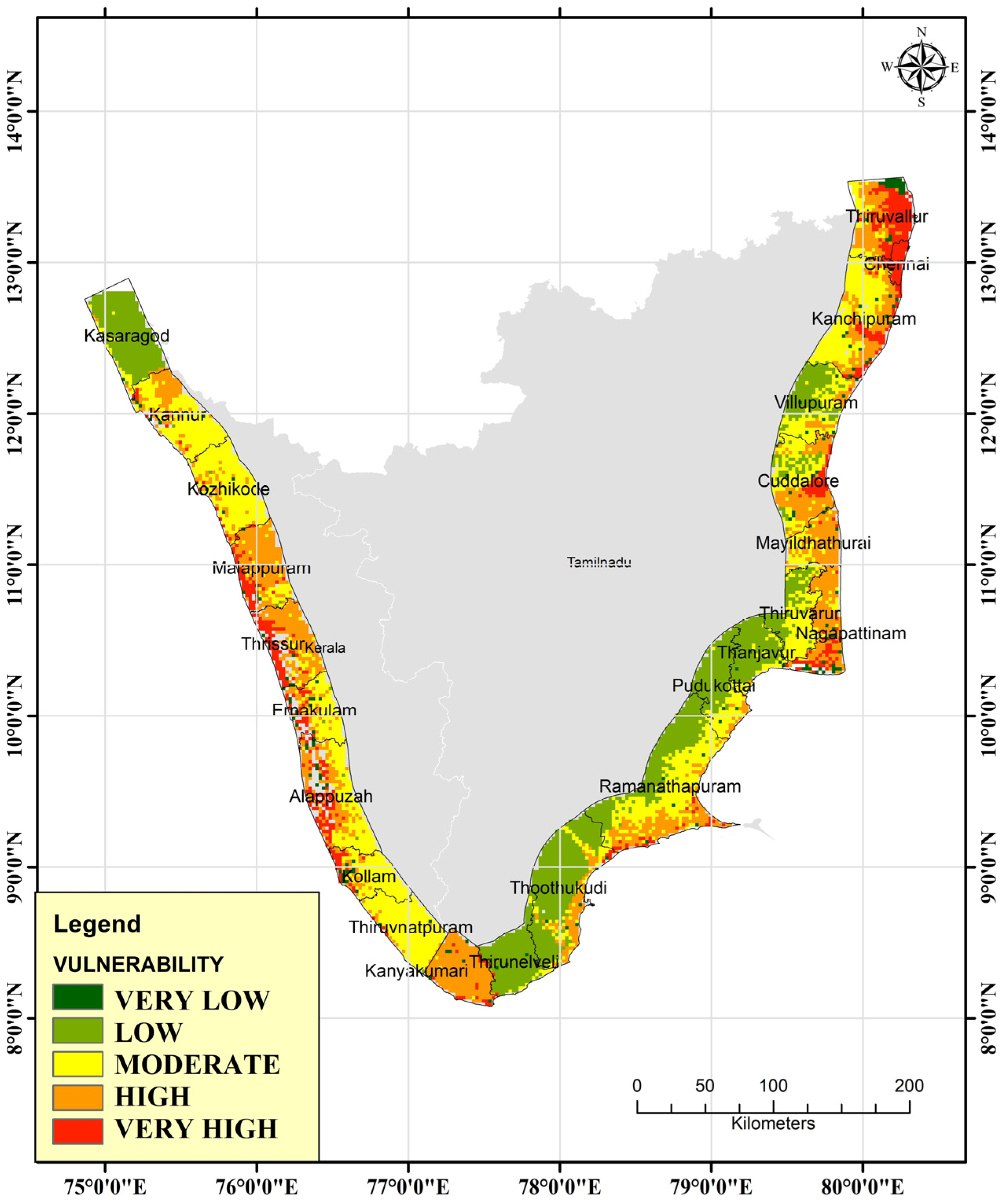
4.5. Overall Vulnerability Assessment
4.6. Comparative Assessment between Tamil Nadu and Kerala Coasts
5. Discussion
6. Conclusions
Author Contributions
Funding
Institutional Review Board Statement
Informed Consent Statement
Data Availability Statement
Acknowledgments
Conflicts of Interest
Appendix A
| Defuzzified Matrix | |||||||
| GEO | RE | MSL | SWH | TIDAL R | SM | ||
| GEO | 1 | 1.33 | 3 | 9 | 8 | 8 | |
| RE | 0.83 | 1 | 5 | 5 | 8 | 8 | |
| MSL | 0.36 | 0.21 | 1 | 3 | 3 | 7 | |
| SWH | 0.11 | 0.21 | 0.4 | 1 | 3 | 5 | |
| TIDAL R | 0.13 | 0.13 | 0.4 | 0.36 | 1 | 1.3 | |
| SM | 0.13 | 0.13 | 0.1 | 0.21 | 0.8 | 1 | |
| TOTALS | 2.56 | 3 | 9.9 | 18.6 | 24 | 30 | |
Appendix B
| Normalized Matrix | ||||||
| GEO | RE | MSL | SWH | SLOPE | SM | |
| GEO | 0.39 | 0.44 | 0.3 | 0.48 | 0.3 | 0.3 |
| RE | 0.33 | 0.33 | 0.5 | 0.27 | 0.3 | 0.3 |
| MSL | 0.14 | 0.07 | 0.1 | 0.16 | 0.1 | 0.2 |
| SWH | 0.04 | 0.07 | 0 | 0.05 | 0.1 | 0.2 |
| SLOPE | 0.05 | 0.04 | 0 | 0.02 | 0 | 0 |
| SM | 0.05 | 0.04 | 0 | 0.01 | 0 | 0 |
Appendix C
| Weights | Weighted Sum | Lambda |
| 0.37066 | 2.535548 | 6.840637 |
| 0.339141 | 2.308372 | 6.806535 |
| 0.138219 | 0.921197 | 6.664763 |
| 0.082198 | 0.514093 | 6.254363 |
| 0.038915 | 0.249332 | 6.407104 |
| 0.030868 | 0.189877 | 6.151184 |
Appendix D
| Validating Parameters | ||
| Lambda Max | 6.520764 | |
| n | 6 | |
| RI | 1.24 | |
| C I | (L-N/N-1) | 0.104153 |
| CR | (CI/RI) | 0.083994 |
References
- Nayak, S. Coastal Zone Management in India—Present Status and Future Needs. Geo Spat. Inf. Sci. 2017, 20, 174–183. [Google Scholar] [CrossRef]
- Ahmad, H. Bangladesh Coastal Zone Management Status and Future Trends. J. Coast. Zone Manag. 2019, 22, 466. [Google Scholar]
- Davidson-Arnott, R.; Bauer, B.; Houser, C. Introduction to Coastal Processes and Geomorphology; Cambridge University Press: Cambridge, UK, 2019; ISBN 9781108424271. [Google Scholar]
- Unnikrishnan, A.S.; Kumar, K.R.; Fernandes, S.E.; Michael, G.S.; Patwardhan, S.K. Sea Level Changes along the Indian Coast: Observations and Projections. Curr. Sci. 2006, 90, 362–368. [Google Scholar]
- Tahri, M.; Maanan, M.; Maanan, M.; Bouksim, H.; Hakdaoui, M. Using Fuzzy Analytic Hierarchy Process Multi-Criteria and Automatic Computation to Analyse Coastal Vulnerability. Prog. Phys. Geogr. Earth Environ. 2017, 41, 268–285. [Google Scholar] [CrossRef]
- Masselink, G.; Hughes, M.; Knight, J. Introduction to Coastal Processes and Geomorphology; Routledge: Oxfordshire, UK, 2014. [Google Scholar]
- Orviku, K.; Jaagus, J.; Kont, A.; Ratas, U. Reimo Rivis Increasing Activity of Coastal Processes Associated with Climate Change in Estonia. J. Coast. Res. 2003, 19, 364–375. [Google Scholar]
- Bird, E. Coastal Geomorphology: An Introduction, 2nd ed.; Wiley-Blackwell: Hoboken, NJ, USA, 2008; ISBN 9780470517291. [Google Scholar]
- Nicholls, R.J.; Klein, R.J.T. Climate Change and Coastal Management on Europe’s Coast. In Managing European Coasts; Springer: Berlin/Heidelberg, Germany, 2005; pp. 199–226. [Google Scholar]
- Kaliraj, S.; Chandrasekar, N.; Ramachandran, K.K. Mapping of Coastal Landforms and Volumetric Change Analysis in the South West Coast of Kanyakumari, South India Using Remote Sensing and GIS Techniques. Egypt J. Remote Sens. Space Sci. 2017, 20, 265–282. [Google Scholar] [CrossRef]
- Basheer Ahammed, K.K.; Pandey, A.C. Geoinformatics Based Assessment of Coastal Multi-Hazard Vulnerability along the East Coast of India. Spat. Inf. Res. 2019, 27, 295–307. [Google Scholar] [CrossRef]
- Serafin, K.A.; Ruggiero, P.; Barnard, P.L.; Stockdon, H.F. The Influence of Shelf Bathymetry and Beach Topography on Extreme Total Water Levels: Linking Large-Scale Changes of the Wave Climate to Local Coastal Hazards. Coast. Eng. 2019, 150, 1–17. [Google Scholar] [CrossRef]
- Parida, B.R.; Behera, S.N.; Oinam, B.; Patel, N.R.; Sahoo, R.N. Investigating the Effects of Episodic Super-Cyclone 1999 and Phailin 2013 on Hydro-Meteorological Parameters and Agriculture: An Application of Remote Sensing. Remote Sens. Appl. Soc. Environ. 2018, 10, 128–137. [Google Scholar] [CrossRef]
- Basheer Ahammed, K.K.; Pandey, A.C.; Parida, B.R.; Wasim; Dwivedi, C.S. Impact Assessment of Tropical Cyclones Amphan and Nisarga in 2020 in the Northern Indian Ocean. Sustainability 2023, 15, 3992. [Google Scholar] [CrossRef]
- Kumar, V.S.; Pathak, K.C.; Pednekar, P.; Raju, N.S.N.; Gowthaman, R. Coastal Processes along the Indian Coastline. Curr. Sci. 2006, 91, 530–536. [Google Scholar]
- Senapati, S.; Gupta, V. Climate Change and Coastal Ecosystem in India: Issues in Perspectives. Int. J. Environ. Sci. 2014, 5, 530–543. [Google Scholar]
- Sheik Mujabar, P.; Chandrasekar, N. Coastal Erosion Hazard and Vulnerability Assessment for Southern Coastal Tamil Nadu of India by Using Remote Sensing and GIS. Nat. Hazards 2013, 69, 1295–1314. [Google Scholar] [CrossRef]
- O’Regan, P.R. The Use of Contemporary Information Technologies for Coastal Research and Management: A Review. J. Coast. Res. 1996, 12, 192–204. [Google Scholar]
- Pantusa, D.; D’Alessandro, F.; Frega, F.; Francone, A.; Tomasicchio, G.R. Improvement of a Coastal Vulnerability Index and Its Application along the Calabria Coastline, Italy. Sci. Rep. 2022, 12, 21959. [Google Scholar] [CrossRef] [PubMed]
- What Is Coastal Vulnerability Index (CVI)?—Civilsdaily. Available online: https://www.civilsdaily.com/news/what-is-coastal-vulnerability-index-cvi/ (accessed on 21 May 2023).
- Hasan, M.U.; Drakou, E.G.; Karymbalis, E.; Tragaki, A.; Gallousi, C.; Liquete, C. Modelling and Mapping Coastal Protection: Adapting an EU-Wide Model to National Specificities. Sustainability 2022, 15, 260. [Google Scholar] [CrossRef]
- Klemas, V. Remote Sensing Techniques for Studying Coastal Ecosystems: An Overview. J. Coast. Res. 2011, 27, 2–17. [Google Scholar]
- Ai, B.; Tian, Y.; Wang, P.; Gan, Y.; Luo, F.; Shi, Q. Vulnerability Analysis of Coastal Zone Based on InVEST Model in Jiaozhou Bay, China. Sustainability 2022, 14, 6913. [Google Scholar] [CrossRef]
- Lu, J.; Zhang, Y.; Shi, H.; Lv, X. Coastal Vulnerability Modelling and Social Vulnerability Assessment under Anthropogenic Impacts. Front. Mar. Sci. 2022, 9, 2038. [Google Scholar] [CrossRef]
- Furlan, E.; Pozza, P.D.; Michetti, M.; Torresan, S.; Critto, A.; Marcomini, A. Development of a Multi-Dimensional Coastal Vulnerability Index: Assessing Vulnerability to Inundation Scenarios in the Italian Coast. Sci. Total Environ. 2021, 772, 144650. [Google Scholar] [CrossRef]
- Valis, D.; Hasilova, K.; Forbelska, M.; Pietrucha-Urbanik, K. Modelling Water Distribution Network Failures and Deterioration. In Proceedings of the 2017 IEEE International Conference on Industrial Engineering and Engineering Management (IEEM), Singapore, 10–13 December 2017; pp. 924–928. [Google Scholar]
- Mullick, M.R.A.; Tanim, A.H.; Islam, S.M.S. Coastal Vulnerability Analysis of Bangladesh Coast Using Fuzzy Logic Based Geospatial Techniques. Ocean Coast. Manag. 2019, 174, 154–169. [Google Scholar] [CrossRef]
- Pantusa, D.; Saponieri, A.; Tomasicchio, G.R. Assessment of Coastal Vulnerability to Land-Based Sources of Pollution and Its Application in Apulia, Italy. Sci. Total Environ. 2023, 886, 163754. [Google Scholar] [CrossRef] [PubMed]
- Wu, C.; Liu, G.; Huang, C.; Liu, Q.; Guan, X. Ecological Vulnerability Assessment Based on Fuzzy Analytical Method and Analytic Hierarchy Process in Yellow River Delta. Int. J. Environ. Res. Public Health 2018, 15, 855. [Google Scholar] [CrossRef] [PubMed]
- Barzehkar, M.; Parnell, K.E.; Soomere, T.; Dragovich, D.; Engström, J. Decision Support Tools, Systems and Indices for Sustainable Coastal Planning and Management: A Review. Ocean Coast. Manag. 2021, 212, 105813. [Google Scholar] [CrossRef]
- Cao, C.; Cai, F.; Qi, H.; Liu, J.; Lei, G.; Zhu, K.; Mao, Z. Coastal Erosion Vulnerability in Mainland China Based on Fuzzy Evaluation of Cloud Models. Front. Mar. Sci. 2022, 8, 790664. [Google Scholar] [CrossRef]
- Hoque, M.A.-A.; Pradhan, B.; Ahmed, N.; Ahmed, B.; Alamri, A.M. Cyclone Vulnerability Assessment of the Western Coast of Bangladesh. Geomat. Nat. Hazards Risk 2021, 12, 198–221. [Google Scholar] [CrossRef]
- Kuriakose, G.; Sebastian, J. History, Biogeography, Biodiversity and Bioprospecting: Scenario from the Western Ghats. South Indian J. Biol. Sci. 2016, 2, 292–301. [Google Scholar] [CrossRef]
- Hegde, S.; Sharathchandra, K.; Sridhar, K.R. Honey-Producing Bee–Pollen–Vegetation Relationships in the West Coast and Western Ghats of India. Palynology 2023, 16, 2127957. [Google Scholar] [CrossRef]
- Hall, K.R. Commodity Flows, Diaspora Networking, and Contested Agency in the Eastern Indian Ocean c. 1000–1500. TRaNS Trans-Reg.-Natl. Stud. Southeast Asia 2016, 4, 387–417. [Google Scholar] [CrossRef]
- Jayappa, K.S.; Mitra, D.; Mishra, A.K. Coastal Geomorphological and Land-use and Land-cover Study of Sagar Island, Bay of Bengal (India) Using Remotely Sensed Data. Int. J. Remote Sens. 2006, 27, 3671–3682. [Google Scholar] [CrossRef]
- Woodcock, C.E.; Allen, R.; Anderson, M.; Belward, A.; Bindschadler, R.; Cohen, W.; Gao, F.; Goward, S.N.; Helder, D.; Helmer, E.; et al. Free Access to Landsat Imagery. Science 2008, 320, 1011. [Google Scholar] [CrossRef] [PubMed]
- USGS; NASA. Landsat Data Users Handbook; USGS and NASA: Reston, VA, USA; p. 8.
- Farr, T.G.; Rosen, P.A.; Caro, E.; Crippen, R. The Shuttle Radar Topography Mission. Rev. Geophys. 2007, 45, 2. [Google Scholar] [CrossRef]
- Werner, M. Shuttle Radar Topography Mission (SRTM): Experience with the X-Band SAR Interferometer. In Proceedings of the 2001 CIE International Conference on Radar Proceedings (Cat No.01TH8559), Beijing, China, 15–18 October 2001; pp. 634–638. [Google Scholar]
- Adilakshmi, L.; Manglik, A.; Thiagarajan, S.; Suresh, M. Crustal Structure of the Indian Plate underneath the Alluvial Plains of the Central Ganga Basin by Broadband Magnetotellurics. Tectonophysics 2021, 802, 228746. [Google Scholar] [CrossRef]
- Tolman, H.L. User Manual and System Documentation of WAVEWATCH III TM Version 3.14. Technical Note, MMAB Contribution. Available online: https://www.google.com.hk/search?q=Tolman+User+Manual+and+System+Documentation+of+WAVEWATCH+III+TM+Version+3.14.+Technical+Note%2C+MMAB+Contribution&ei=7DeJZM_8G8XChwORoqj4Ag&ved=0ahUKEwjPos_M7MH_AhVF4WEKHRERCi8Q4dUDCA4&uact=5&oq=Tolman+User+Manual+and+System+Documentation+of+WAVEWATCH+III+TM+Version+3.14.+Technical+Note%2C+MMAB+Contribution&gs_lcp=Cgxnd3Mtd2l6LXNlcnAQA0oECEEYAFAAWABgAGgAcAB4AIABAIgBAJIBAJgBAKABAqABAQ&sclient=gws-wiz-serp (accessed on 21 May 2023).
- Duong, T.M.; Ranasinghe, R.; Thatcher, M.; Mahanama, S.; Wang, Z.B.; Dissanayake, P.K.; Hemer, M.; Luijendijk, A.; Bamunawala, J.; Roelvink, D.; et al. Assessing climate change impacts on the stability of small tidal inlets: Part 2- data rich environments. Mar. Geol. 2018, 395, 65–81. [Google Scholar] [CrossRef] [PubMed]
- Merrifield, M.; Aarup, T.; Allen, A.; Aman, A.; Caldwell, P.; Bradshaw, E.; Fernandes, R.M.S.; Hayashibara, H.; Hernandez, F.; Kilonsky, B.; et al. The Global Sea Level Observing System (GLOSS). In Proceedings of the Ocean Obs, Venice, Italy, 25 September 2009; p. 9. [Google Scholar]
- Bell, C.; Vassie, J.M.; Woodworth, P.L. POL/PSMSL Tidal Analysis Software Kit 2000 (TASK-2000). In Permanent Service for Mean Sea Level; Bidston Observatory: Birkenhead, UK, 1999; p. 20. [Google Scholar]
- Gao, J.; Pesaresi, M. Downscaling SSP-consistent global spatial urban land projections from 1/8-degree to 1-km resolution 2000–2100. Sci. Data 2021, 8, 281. [Google Scholar] [CrossRef] [PubMed]
- Naga Kumar, K.C.V.; Deepak, P.M.; Basheer Ahammed, K.K.; Rao, K.N.; Gopinath, G.; Dinesan, V.P. Coastal Vulnerability Assessment Using Geospatial Technologies and a Multi-Criteria Decision Making Approach—A Case Study of Kozhikode District Coast, Kerala State, India. J. Coast. Conserv. 2022, 26, 16. [Google Scholar] [CrossRef]
- Shared Socioeconomic Pathways (SSPs). Available online: https://sedac.ciesin.columbia.edu/data/set/ssp-1-km-downscaled-urban-land-extent-projection-base-year-ssp-2000-2100 (accessed on 25 September 2022).
- Priya Rajan, S.M.; Nellayaputhenpeedika, M.; Tiwari, S.P.; Vengadasalam, R. Mapping and Analysis of the Physical Vulnerability of Coastal Tamil Nadu. Hum. Ecol. Risk Assess. Int. J. 2020, 26, 1879–1895. [Google Scholar] [CrossRef]
- Arkema, K.K.; Guannel, G.; Verutes, G.; Wood, S.A.; Guerry, A.; Ruckelshaus, M.; Kareiva, P.; Lacayo, M.; Silver, J.M. Coastal Habitats Shield People and Property from Sea-Level Rise and Storms. Nat. Clim. Chang. 2013, 3, 913–918. [Google Scholar] [CrossRef]
- Hadipour, V.; Vafaie, F.; Kerle, N. An Indicator-Based Approach to Assess Social Vulnerability of Coastal Areas to Sea-Level Rise and Flooding: A Case Study of Bandar Abbas City, Iran. Ocean Coast. Manag. 2020, 188, 105077. [Google Scholar] [CrossRef]
- Rajakumari, S.; Minnu, A.; Sarunjith, K.J. Determination of Vulnerable Zones along Brahmapur Coast, Odisha Using AHP and GIS with Validation against Multiple Cyclones. Environ. Monit. Assess. 2022, 194, 278. [Google Scholar] [CrossRef]
- Baig, M.R.I.; Shahfahad; Ahmad, I.A.; Tayyab, M.; Asgher, M.S.; Rahman, A. Coastal Vulnerability Mapping by Integrating Geospatial Techniques and Analytical Hierarchy Process (AHP) along the Vishakhapatnam Coastal Tract, Andhra Pradesh, India. J. Indian Soc. Remote Sens. 2021, 49, 215–231. [Google Scholar] [CrossRef]
- Dwarakish, G.S.; Vinay, S.A.; Natesan, U.; Asano, T.; Kakinuma, T.; Venkataramana, K.; Pai, B.J.; Babita, M.K. Coastal Vulnerability Assessment of the Future Sea Level Rise in Udupi Coastal Zone of Karnataka State, West Coast of India. Ocean Coast. Manag. 2009, 52, 467–478. [Google Scholar] [CrossRef]
- Sankari, T.S.; Chandramouli, A.R.; Gokul, K.; Surya, S.S.M.; Saravanavel, J. Coastal Vulnerability Mapping Using Geospatial Technologies in Cuddalore-Pichavaram Coastal Tract, Tamil Nadu, India. Aquat. Procedia 2015, 4, 412–418. [Google Scholar] [CrossRef]
- Ghosh, S.; Mistri, B. Assessing Coastal Vulnerability to Environmental Hazards of Indian Sundarban Delta Using Multi-Criteria Decision-Making Approaches. Ocean Coast. Manag. 2021, 209, 105641. [Google Scholar] [CrossRef]
- Mani Murali, R.; Ankita, M.; Amrita, S.; Vethamony, P. Coastal Vulnerability Assessment of Puducherry Coast, India, Using the Analytical Hierarchical Process. Nat. Hazards Earth Syst. Sci. 2013, 13, 3291–3311. [Google Scholar] [CrossRef]
- Mahapatra, M.; Ramakrishnan, R.; Rajawat, A.S. Coastal Vulnerability Assessment Using Analytical Hierarchical Process for South Gujarat Coast, India. Nat. Hazards 2015, 76, 139–159. [Google Scholar] [CrossRef]
- Le Cozannet, G.; Garcin, M.; Bulteau, T.; Mirgon, C.; Yates, M.L.; Méndez, M.; Baills, A.; Idier, D.; Oliveros, C. An AHP-Derived Method for Mapping the Physical Vulnerability of Coastal Areas at Regional Scales. Nat. Hazards Earth Syst. Sci. 2013, 13, 1209–1227. [Google Scholar] [CrossRef]
- Lin, L.; Pussella, P. Assessment of Vulnerability for Coastal Erosion with GIS and AHP Techniques Case Study: Southern Coastline of Sri Lanka. Nat. Resour. Model. 2017, 30, e12146. [Google Scholar] [CrossRef]
- Behera, R.; Kar, A.; Das, M.R.; Panda, P.P. GIS-Based Vulnerability Mapping of the Coastal Stretch from Puri to Konark in Odisha Using Analytical Hierarchy Process. Nat. Hazards 2019, 96, 731–751. [Google Scholar] [CrossRef]
- Kumar, T.S.; Mahendra, R.S.; Nayak, S. Coastal Vulnerability Assessment for Orissa State, East Coast of India. J. Coast. 2010, 26, 523–534. [Google Scholar] [CrossRef]
- Nageswara Rao, K.; Subraelu, P.; Venkateswara Rao, T.; Hema Malini, B.; Ratheesh, R.; Bhattacharya, S.; Rajawat, A.S. Ajai Sea-Level Rise and Coastal Vulnerability: An Assessment of Andhra Pradesh Coast, India through Remote Sensing and GIS. J. Coast. Conserv. 2008, 12, 195–207. [Google Scholar] [CrossRef]
- Sudha Rani, N.N.V.; Satyanarayana, A.N.V.; Bhaskaran, P.K. Coastal Vulnerability Assessment Studies over India: A Review. Nat. Hazards 2015, 77, 405–428. [Google Scholar] [CrossRef]
- Arun Kumar, A.; Kunte, P.D. Coastal Vulnerability Assessment for Chennai, East Coast of India Using Geospatial Techniques. Nat. Hazards 2012, 64, 853–872. [Google Scholar] [CrossRef]
- Kumar, R.; Dwivedi, S.B.; Gaur, S. A Comparative Study of Machine Learning and Fuzzy-AHP Technique to Groundwater Potential Mapping in the Data-Scarce Region. Comput. Geosci. 2021, 155, 104855. [Google Scholar] [CrossRef]


| State | SL. NO | Coastal District | East West Extent (km) | Coastal Extent (East/West) (km) |
|---|---|---|---|---|
| TAMIL NADU | 1 | THIRUVALLUR | 118 | E 59 |
| 2 | CHENNAI | 18 | E 9 | |
| 3 | CHENGALPATTU | 50 | E 25 | |
| 4 | VILLUPURAM | 90 | E 45 | |
| 5 | CUDDALORE | 100 | E 50 | |
| 6 | MAYILDATURAI | 36 | E 18 | |
| 7 | NAGAPATTNAM | 65 | E 32.5 | |
| 8 | THANJAVUR | 90 | E 45 | |
| 9 | PADUKOTTAI | 108 | E 54 | |
| 10 | RAMANATHAPURAM | 140 | E 70 | |
| 11 | THOOTHUKUDI | 98 | E 49 | |
| 12 | THIRUNELVELI | 96 | E 48 | |
| 13 | KANYAKUMARI | 59 | E 29.5 | |
| AVERAGE | 82.15 | 41.08 | ||
| KERALA | 14 | KASARAGOD | 38 | W 19 |
| 15 | KANNUR | 80 | W 40 | |
| 16 | KOZHIKODE | 56 | W 28 | |
| 17 | MALLAPPURAM | 88 | W 44 | |
| 18 | THRISSUR | 98 | W 49 | |
| 19 | ERNAKULAM | 98 | W 49 | |
| 20 | ALAPPUZAH | 30 | W 15 | |
| 21 | KOLLAM | 75 | W 37.5 | |
| 22 | THIRUVANANTHAPURAM | 72 | W 36 | |
| AVERAGE | 70.56 | 35.28 |
| Dataset | Source | Type | Resolution | Year | Month |
|---|---|---|---|---|---|
| Landsat 5, 8, and 9 | USGS | MSS Raster | 30 m | 1990–2022 | Nov–Dec |
| Geomorphology 1:250 K | Bhukosh GSI | Shapefile | 250 m | 2015 | - |
| SRTM | Earthdata | Geo tiff | 30 m | 2000 | - |
| WAVE WATCH III | APDRC | NetCDF | 3 h | 1997–2019 | Annual |
| GLOSS–PSMSL | PSMSL | Text | - | 1990–2020 | Annual |
| Population | SEDAC | Raster | 1 km | 2011 | - |
| Built-up | SEDAC | Shapefile | 250 m | 2011 | - |
| Parameter | Geomorphology (GEO) | Regional Elevation (RE) | Mean Sea Level Rise (MSL) | Surface Sig’ Wave Height (SWH) | Slope | Shoreline Movement (SM) | Weights | ||||||||||||
|---|---|---|---|---|---|---|---|---|---|---|---|---|---|---|---|---|---|---|---|
| GEO | 1 | 1 | 1 | 1 | 1 | 2 | 2 | 3 | 4 | 9 | 9 | 9 | 7 | 8 | 9 | 7 | 8 | 9 | 0.37066 |
| RE | 0.5 | 1 | 1 | 1 | 1 | 1 | 4 | 5 | 6 | 4 | 5 | 6 | 7 | 8 | 9 | 7 | 8 | 9 | 0.33066 |
| MSL | 0.25 | 0.33 | 0.50 | 0.17 | 0.20 | 0.25 | 1 | 1 | 1 | 2 | 3 | 4 | 2 | 3 | 4 | 6 | 7 | 8 | 0.13829141 |
| SWH | 0.11 | 0.11 | 0.11 | 0.17 | 0.20 | 0.25 | 0.25 | 0.33 | 0.50 | 1 | 1 | 1 | 2 | 3 | 4 | 4 | 5 | 6 | 0.082198 |
| Slope | 0.11 | 0.13 | 0.14 | 0.11 | 0.13 | 0.14 | 0.25 | 0.33 | 0.50 | 0.25 | 0.33 | 0.50 | 1 | 1 | 1 | 1 | 1 | 2 | 0.038915 |
| SM | 0.11 | 0.13 | 0.14 | 0.11 | 0.13 | 0.14 | 0.13 | 0.14 | 0.17 | 0.17 | 0.20 | 0.25 | 0.5 | 1 | 1 | 1 | 1 | 1 | 0.030868 |
| Scale | Very High Vulnerability (VHV) | High Vulnerability (HV) | Medium Vulnerability (MV) | Low Vulnerability (LV) | Very Low Vulnerability (VLV) | ||||||||||
|---|---|---|---|---|---|---|---|---|---|---|---|---|---|---|---|
| VHV | 1 | 1 | 1 | 1 | 1 | 2 | 2 | 3 | 4 | 4 | 5 | 6 | 7 | 8 | 9 |
| HV | 0.5 | 1 | 1 | 1 | 1 | 1 | 2 | 3 | 4 | 4 | 5 | 6 | 7 | 8 | 9 |
| MV | 0.25 | 0.33 | 0.50 | 0.25 | 0.33 | 0.50 | 1 | 1 | 1 | 2 | 3 | 4 | 4 | 5 | 6 |
| LV | 0.17 | 0.20 | 0.225 | 0.17 | 0.20 | 0.25 | 0.25 | 0.33 | 0.50 | 1 | 1 | 1 | 2 | 3 | 4 |
| VLV | 0.11 | 0.13 | 0.14 | 0.11 | 0.13 | 0.14 | 0.17 | 0.20 | 0.25 | 0.25 | 0.33 | 0.50 | 1 | 1 | 1 |
| Parameter | VHV | HV | MV | LV | VLV |
|---|---|---|---|---|---|
| GEO | Coastal plain | Deltaic plain | Flood plain | Water bodies | PPC and hills |
| RE | <3 m | 4 to 6 m | 7 to 12 m | 12 to 18 m | >18 m |
| SLR | >3.16 cm | 2.96 to 3.16 cm | 2.51 to 2.95 cm | 1.81 to 2.5 | <1.8 cm |
| SWH Slope SB | >1.2 m 0–10 degrees Very high erosion | 0.9 to 1.2 m 10–20 degrees High Erosion | 0.6 to 0.9 m 20–45 degrees High Accretion | 0.3 to 0.6 m 45–60 degrees VH Accretion | <0.3 m 60–89 degrees No Change |
| PD | >1000 ppl/km2 | 500–1000 | 250–500 | 100–250 | <100 |
| Built-up density | 80–100% | 40–80% | 20–40% | 10–20% | <10% |
| Urban density | >400 hh/km2 | 200–400 | 100–200 | 50–100 | <50 |
| Parameter | Classes | Tamil Nadu Coast (km2) | % | Kerala Coast (km2) | % |
|---|---|---|---|---|---|
| Geomorphology | Coastal plains | 4257.29 | 13.51 | 2395.23 | 12.53 |
| Deltaic plains | 8509.73 | 27.00 | 494.24 | 2.59 | |
| Flood plains | 1712.55 | 5.43 | 787.62 | 4.12 | |
| Waterbody | 3112.13 | 9.87 | 432.03 | 2.26 | |
| Pediment–pediplain complex and hills | 13,928.00 | 44.19 | 15,009.70 | 78.51 | |
| Sea level rise | <1.8 mm | 25,000.50 | 79.24 | 2874.99 | 14.92 |
| 1.81–2.25 mm | 6548.64 | 20.76 | 16,394.00 | 85.08 | |
| Significant wave height | <0.3 m | 9153.76 | 29.06 | 19,071.30 | 100.00 |
| 0.3–0.6 m | 19,333.40 | 61.37 | - | 0 | |
| 0.6–0.9 m | 3017.09 | 9.58 | - | 0 | |
| Physical vulnerability | Very low | 638.05 | 2.10 | 404.50 | 2.35 |
| Low | 6650.20 | 21.93 | 13,983.20 | 81.08 | |
| Moderate | 10,734.20 | 35.40 | 2454.54 | 14.23 | |
| High | 8047.80 | 26.54 | 404.46 | 2.35 | |
| Very high | 54.07 | 14.03 | - | 0 | |
| Social vulnerability | Very low | 8486.12 | 18.70 | - | 0 |
| Low | 14,078.60 | 31.02 | 2100.32 | 12.15 | |
| Moderate | 5111.56 | 11.26 | 143.31 | 0.83 | |
| High | 9822.65 | 21.65 | 9782.78 | 56.61 | |
| Very high | 7881.63 | 17.37 | 5254.76 | 30.41 | |
| Overall vulnerability | Very low | 968.88 | 3.22 | 497.42 | 2.90 |
| Low | 10,869.96 | 36.13 | 2015.82 | 11.73 | |
| Moderate | 8630.94 | 28.69 | 9430.49 | 54.89 | |
| High | 7421.68 | 24.67 | 3691.11 | 21.48 | |
| Very high | 2194.55 | 7.29 | 1545.12 | 8.99 | |
| Shoreline behavior | High accretion | 302.63 km | 31.91 | 316.26 km | 56.57 |
| High erosion | 591.55 km | 62.38 | 242.82 km | 43.43 | |
| Very high erosion | 54.07 km | 5.70 | - | 0 |
Disclaimer/Publisher’s Note: The statements, opinions and data contained in all publications are solely those of the individual author(s) and contributor(s) and not of MDPI and/or the editor(s). MDPI and/or the editor(s) disclaim responsibility for any injury to people or property resulting from any ideas, methods, instructions or products referred to in the content. |
© 2023 by the authors. Licensee MDPI, Basel, Switzerland. This article is an open access article distributed under the terms and conditions of the Creative Commons Attribution (CC BY) license (https://creativecommons.org/licenses/by/4.0/).
Share and Cite
Dwivedi, C.S.; Pampattiwar, S.T.; Pandey, A.C.; Parida, B.R.; Mitra, D.; Kumar, N. Characterization of the Coastal Vulnerability in Different Geological Settings: A Comparative Study on Kerala and Tamil Nadu Coasts Using FuzzyAHP. Sustainability 2023, 15, 9543. https://doi.org/10.3390/su15129543
Dwivedi CS, Pampattiwar ST, Pandey AC, Parida BR, Mitra D, Kumar N. Characterization of the Coastal Vulnerability in Different Geological Settings: A Comparative Study on Kerala and Tamil Nadu Coasts Using FuzzyAHP. Sustainability. 2023; 15(12):9543. https://doi.org/10.3390/su15129543
Chicago/Turabian StyleDwivedi, Chandra Shekhar, Shiva Teja Pampattiwar, Arvind Chandra Pandey, Bikash Ranjan Parida, Debashis Mitra, and Navneet Kumar. 2023. "Characterization of the Coastal Vulnerability in Different Geological Settings: A Comparative Study on Kerala and Tamil Nadu Coasts Using FuzzyAHP" Sustainability 15, no. 12: 9543. https://doi.org/10.3390/su15129543
APA StyleDwivedi, C. S., Pampattiwar, S. T., Pandey, A. C., Parida, B. R., Mitra, D., & Kumar, N. (2023). Characterization of the Coastal Vulnerability in Different Geological Settings: A Comparative Study on Kerala and Tamil Nadu Coasts Using FuzzyAHP. Sustainability, 15(12), 9543. https://doi.org/10.3390/su15129543