Machine Learning-Based Land Use and Land Cover Mapping Using Multi-Spectral Satellite Imagery: A Case Study in Egypt

Abstract

Satellite images provide continuous access to observations of the Earth, making environmental monitoring more convenient for certain applications, such as tracking changes in land use and land cover (LULC). This paper is aimed to develop a prediction model for mapping LULC using multi-spectral satellite images, which were captured at a spatial resolution of 3 m by a 4-band PlanetScope satellite. The dataset used in the study includes 105 geo-referenced images categorized into 8 LULC different classes. To train this model on both raster and vector data, various machine learning strategies such as Support Vector Machines (SVMs), Decision Trees (DTs), Random Forests (RFs), Normal Bayes (NB), and Artificial Neural Networks (ANNs) were employed. A set of metrics including precision, recall, F-score, and kappa index are utilized to measure the accuracy of the model. Empirical experiments were conducted, and the results show that the ANN achieved a classification accuracy of 97.1%. To the best of our knowledge, this study represents the first attempt to monitor land changes in Egypt that were conducted on high-resolution images with 3 m of spatial resolution. This study highlights the potential of this approach for promoting sustainable land use practices and contributing to the achievement of sustainable development goals. The proposed method can also provide a reliable source for improving geographical services, such as detecting land changes.

1. Introduction

Currently, satellites have Earth look like one compact entity by providing continuous images with fine details [1]. This facility has enabled various applications such as those for agriculture, traffic control, and urban development to be actualized in real time [2]. However, these data need to be processed to infer their semantics. One of these applications is classifying land cover [1]. Land cover is a term used to describe the top layer of the ground, such as water, vegetation, bare soil, urban infrastructure, or another surface covering [3]. The associated processes (e.g., identifying, delineating, and mapping) are crucial for various applications such as global monitoring studies, resource management, and planning activities [4]. To achieve these goals, the first step is to obtain land cover identificationthat allows monitoring activities (e.g., change detection). This also provides information on ground cover for thematic maps’ to learn [3].

Multi-spectral images are images that are composed of data collected from multiple spectral bands or channels of the electromagnetic spectrum. These bands include visible light (red, green, and blue), near-infrared, shortwave infrared, thermal infrared, and others. By collecting data from multiple spectral bands, multi-spectral images can provide information on a variety of surface features, including vegetation health, soil moisture, land use and land cover, and temperature [5]. Applications for these images include mapping of land use and land cover, agricultural monitoring, urban planning, and environmental monitoring. Multi-spectral images are often processed and analyzed using image processing techniques, such as spectral unmixing, classification, and change detection, to extract meaningful pieces of information from the data [6,7].

On the other hand, land use classification aims to define the purpose/function of the land, such as for recreation, wildlife habitat, agriculture, etc. [8]. It draws attention to some applications such as baseline mapping and subsequent monitoring; for instance, the current amount of available land, its type of use, and its changes from year to year [8,9].

Notably, these applications are data- and location-dependent, e.g., land cover and land use vary from place to place because some have problems with illegal use or extinction, such as coastal areas. While most previous studies used pixel-based satellite images to learn Land Use/Land Cover (LULC) classifications, others categorized images as object-based ones. In this research, vector data are used for an object-based “polygon” and raster as a point-based “pixel” to obtain a high-performance classification model [10,11]. Furthermore, unlike previous methods, high-resolution satellite images that offer fine details that can denote the smallest image details are used. As deep learning has advanced, great progress in every field [12,13,14,15], including land cover has witnessed significant improvements [10]. In remote sensing, deep learning has been used in different forms such as LULC change detection [3,4], prediction of LULC [16], dataset and deep learning benchmark [17], image classification of agricultural surfaces [8,9], monitoring of pedestrian detection [10], classification of spatial trajectories [11], and forecasting traffic conditions [18]. Remote sensing, on the other hand, is involved with scanning the Earth using a group of satellites. Deep learning models rely extensively on large-scale datasets. In addition to its usefulness in monitoring land use and land cover changes, predicting LULC can contribute to sustainability efforts. By accurately predicting LULC changes, decision-makers can better plan for sustainable land use practices and mitigate negative impacts on the environment. This information can also be used to inform policies related to conservation, natural resource management, and urban planning. The use of high-resolution satellite imagery for environmental monitoring can also reduce the need for ground-based surveys and inspections, which can be time-consuming, expensive, and potentially harmful to natural habitats. Overall, the integration of satellite imagery and deep learning models can support sustainable development by providing timely and accurate information about changes to the environment.

For these two purposes, a new approach for mapping land use and land cover (LULC) is suggested in this paper, which integrates both raster and vector data using deep learning techniques. The aim of the model is to enhance the precision and effectiveness of LULC mapping, a critical factor in applications such as urban planning and environmental monitoring.

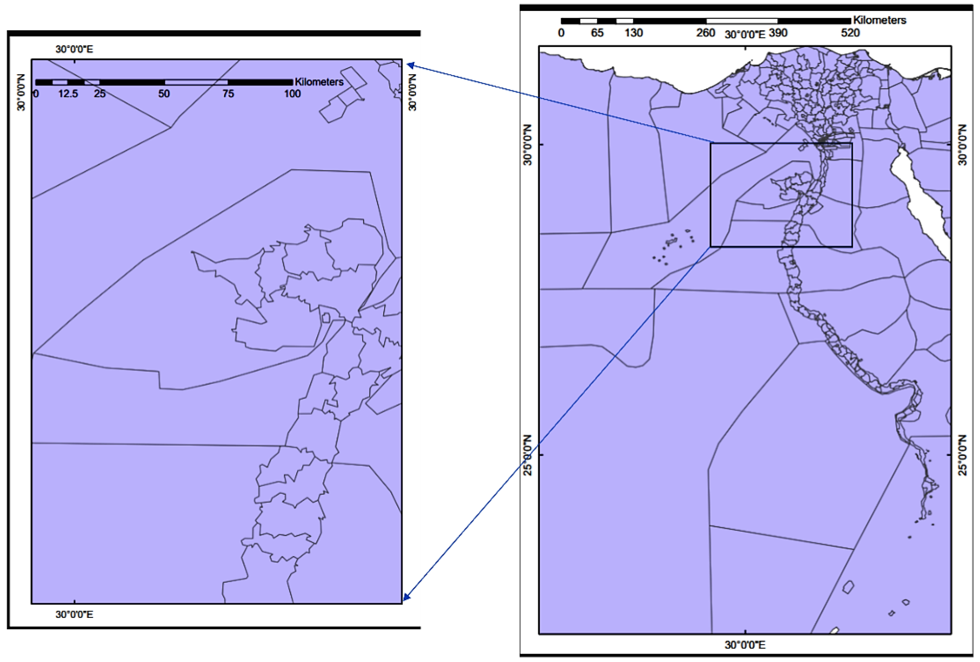
Furthermore, this paper introduces a new dataset for identifying land use and land cover in Fayoum state, Egypt. This state is used as a case study because it has a variety of land use and land cover examples; additional information regarding the geographic location being studied is provided within the “Study Area” Section 3.1. Satellite images are obtained using the 4-band planet scope of 1 June 2022, with each image having 4 bands (red, green, blue, and near-infrared). The ground sample distance for these images is $3.7$ m and their pixel dimensions are $7939\times 3775$. These images undergo a series of procedures before being utilized as input for the proposed model. 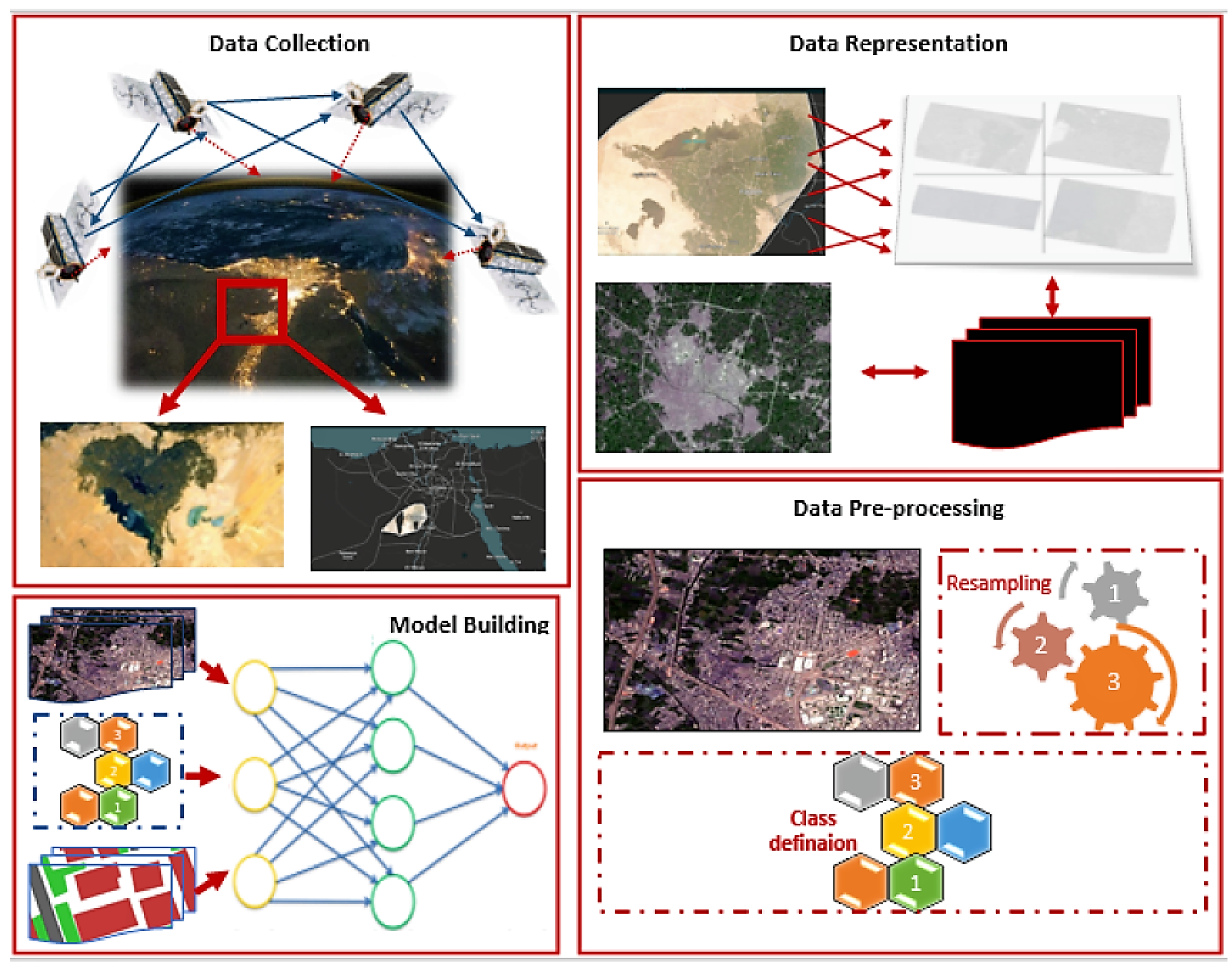Figure 1 illustrates the sequential processes and phases utilized for constructing the model, beginning with data collection from satellite imagery. It then proceeds to data representation, followed by pre-processing to enhance the input images and establish various classes, such as numbers 1, 2, and 3, to represent different categories. Finally, the model building phase is conducted to construct the model using the training data.

Extensive comparisons of the proposed dataset using several models are conducted, with the proposed one trained on two types of data: raster, i.e., high-resolution images, and vector data. Furthermore, we present full benchmarks that demonstrate reliable classification performance and serve as the foundation for developing many applications in the aforementioned domains. How the categorization model may be used to detect changes in land use and/or cover, as well as how it can help improve geographic maps is demonstrated.

The contributions through this work can be summarized as follows:

• Developing a land use and land cover (LULC) model using deep learning that involves utilizing raster and vector data as inputs;
• Proposing a novel large-scale dataset with multi-spectral high-resolution satellite images along with raster data for Fayoum state, Egypt;
• Providing benchmarks for the collected dataset using deep learning/machine learning models;
• Comparing related methods for classifying land cover and land use;
• Comparing between deep learning and machine learning models that accurately classify different types of LULC from satellite imagery;
• Generating a map that shows the various types of land cover and land use in a particular area that involves using remote sensing data and GIS.

2. Related Work

Recent studies have employed deep learning to predict various types of LULC classifications. Some studies were primarily concerned with identifying objects, while others focused specifically on land use and cover.

Venter, Z.S. in [19] compared and evaluated the accuracy and suitability of three global land use and land cover (LULC) maps. The authors have used ground truth data to assess the accuracy of these maps, and have also discussed their relative advantages and disadvantages. The study found that the three LULC maps show strong spatial correspondence for water, built area, tree, and crop classes. However, each map was found to have certain biases in mapping other LULC classes. For instance, Dynamic World (DW) overestimated grass cover, Esri overestimated shrub and scrub cover, and DW overestimated snow and ice cover. In terms of overall accuracy, Esri was found to be the most accurate, followed by DW and World Cover (WC). The most precisely mapped category was water, succeeded by built-up areas, tree cover, and crops. The classes with the lowest accuracies included scrub and shrub, bare ground, grass, and flooded vegetation. The datasets used in this study include DW, WC, and Esri Land Cover (ELC) datasets. DW is a global 10 m resolution LULC dataset developed by the Chinese Academy of Sciences, covering 2015. WC is a global 10 m resolution LULC dataset developed by the European Space Agency, covering 2019. ELC is a global 10 m resolution LULC dataset developed by Esri, covering 2020. The study also found that the accuracy of the LULC maps varied depending on the spatial scale of the ground truth data used. WC was found to have the highest accuracy when European ground truth data from the Land Use/Cover Area Frame Survey (LUCAS) were used, which had a smaller minimum mapping unit than the global ground truth data used in the study. This implies that WC is more suitable for resolving landscape features in greater detail when compared to DW and Esri.

The authors have highlighted the advantages of DW, which offers frequent and near real-time data delivery of categorical predictions and class probability scores. However, they caution that the suitability of global LULC products should be carefully evaluated based on the intended application, such as monitoring aggregate changes in ecosystem accounting versus site-specific change detection. They emphasized the significance of following best practices in design-based inference and area estimation to accurately quantify uncertainty for a specific study area

The major LULC classes of the Athabasca River watershed were found to be coniferous forest (47.30%), agriculture (6.37%), mixed forest (6.65%), water (6.10%), deciduous forest (16.76%), and developed land (3.78%). The study also performed data fusion techniques using the Alberta merged wetland inventory 2017 data to fulfill the data requirements of scientists across a range of disciplines. The data fusion provided two maps which are applicable for hydro-ecological applications, describing two specific categories including different types of burned and wetland classes.

Sertel, E. et al. in [20] discussed the use of deep learning-based segmentation approaches for LULC mapping using very high-resolution (VHR) satellite images. The authors highlighted the increasing importance of LULC mapping in various geospatial applications and the challenges associated with it due to the complexity of LULC classes. A novel benchmark dataset was created by the authors using VHR Worldview-3 images. This dataset has twelve unique LULC classes from two separate geographical areas. Then, the performance of several segmentation architectures and encoders was evaluated to determine the ideal layout for producing extremely precise LULC maps. The metrics used for evaluation included Intersection over Union (IoU), F-1 score, precision, and recall. The most optimal performance across several metric values was achieved by the DeepLabv3+ architecture combined with a ResNeXt50 encoder, which yielded an IoU of 89.46%, an F-1 score of 94.35%, a precision of 94.25%, and a recall of 94.49%. These results demonstrate the potential of deep learning-based segmentation approaches for accurate LULC mapping using VHR satellite images. The authors also propose that supervised, semi-supervised, or weakly supervised deep learning models may be utilized to create new segmentation algorithms using their benchmark dataset as a reference. They may also utilize the model findings to generalize other approaches and transfer learning, providing a valuable resource for future research in this field.

Ali, K. et al. in [21] discuss the use of deep learning methods for LULC classification in semi-arid regions using remote sensing imagery with a medium level of resolution. The authors emphasize the value of comprehensive LULC data for a variety of applications such as urban and rural planning, disaster management, and climate change adaptation. They observed that LULC classification has undergone a paradigm change with the rise of deep learning techniques, and they aimed to assess the efficacy of various Sentinel-2 image band combinations for LULC mapping in semi-arid regions using CNN models.

The results demonstrated that the four-band CNN model exhibits robustness in areas with semi-arid climates, even when dealing with a land cover that is complex in both spectral and spatial aspects. The results also revealed that the ten-band composite did not improve the overall accuracy of the classification, suggesting that using fewer bands may be sufficient for LULC mapping in semi-arid regions.

In [4], Allama, M. et al. examined how remote sensing and GIS techniques can be utilized to monitor changes in land use and land cover within the arid region of Fayoum, Egypt. The authors focused on the period between 1990 and 2018 to analyze the changes that occurred during this time and to identify the driving factors of these changes. The authors used Landsat satellite imagery and a supervised classification approach to categorize the LULC types in the study region. The authors used 4 Landsat images acquired in 1990, 2000, 2010, and 2018 to monitor changes in LULC over time. The study area was classified into six LULC classes, including cultivated land, barren land, water bodies, built-up areas, dunes, and vegetation. The authors used a supervised classification method to classify the Landsat images into four major LULC categories: agriculture, water bodies, urban areas, and bare land. They used the maximum likelihood classifier (MLC) to assign each pixel to one of the four classes based on the spectral signature of the pixel. The authors also used the Normalized Difference Vegetation Index (NDVI) to identify vegetation cover in the study area. The study’s findings demonstrated that LULC in the Fayoum Region has changed significantly over the study period. The authors found that agricultural areas and urban areas had expanded at the expense of water bodies and bare land. They also observed that the NDVI had decreased over time, indicating a decline in vegetation cover.

In [9], a new convolutional neural network (CNN) model called the Weight Feature Value CNN (WFCNN) was developed to conduct remote sensing image segmentation and extract more comprehensive land use information from the images. It comprised an encoder, a classifier, and a set of spectral features, as well as five semantic feature tiers acquired through the encoder. The model utilized linear fusion to hierarchically merge semantic characteristics, while an adjustment layer was employed to fine-tune them for optimal results. The model’s pixel-by-pixel segmentation outperformed other versions in terms of precision, accuracy, recall, and F1-score, indicating its potential advantages. They found that WFCNN can enhance the accuracy and automation of large-scale land use mapping and the extraction of other information using remote sensing imagery. The results indicated that there have been significant changes in LULC in the study area over the last three decades. The analysis showed that the built-up area grew from 0.79% percent in 1990 to 6.35% percent in 2018, while the cultivated land decreased from 32.48% in 1990 to 17.94% in 2018. The results also showed an increase in barren land and sand dunes, which might be attributed to the expansion of urban areas and the over-exploitation of natural resources.

Rousset, G. et al. in [22], aimed to identify the ideal deep learning configuration for LULC mapping in New Caledonia’s complicated subtropical climate. Five sample locations of New Caledonia were labeled by a human operator for a specific dataset based on SPOT6 satellite data, with four serving as training sets and the fifth as a test set. Multiple architectures were trained and evaluated against a cutting-edge machine learning technique and XGBoost. The authors also evaluated the usefulness of common neo-channels that were generated from the raw data in the context of deep learning. The results indicated that the deep learning approach achieved results that were similar to XGBoost for land cover detection while surpassing it for the task of land use detection. Additionally, the accuracy of the deep learning land use classification task was significantly increased by combining the output of the dedicated deep learning architecture’s land cover classification task with the raw channel’s input, achieving an overall accuracy on the LC and LU detection tasks of 61.45% and 51.56%, respectively.

3. Materials and Methods

3.1. Study Area

Fayoum is located in the western region of Egypt, approximately 80 km southwest of Cairo. As depicted in Figure 2, the geographical location can be identified by the coordinates of 29${}^{\circ }$18${}^{\prime }$35.82${}^{″}$ N latitude and 30${}^{\circ }$50${}^{\prime }$30.48${}^{″}$ E longitude. It is recognized for its magnificent natural landscapes and its historical significance, dating back to ancient times. In terms of land use and cover, Fayoum is largely dependent on agriculture, with a significant portion of the surrounding areas comprising expansive farmland. The location’s rich soil and the proximity to the Nile River render it an optimal location for farming, with crops such as wheat, corn, and fruit being cultivated in ample amounts. Furthermore, the city is home to many protected natural sites, such as the Wadi El Rayan and Qarun Lake Protected Areas, which attract many nature lovers and tourists. The surrounding land in the region features land cover types such as urban areas and desert landscapes. Furthermore, there is a mixture of modern and traditional architecture, and it is renowned for its vibrant markets and ancient ruins, drawing tourists from around the globe.

3.2. Dataset and Building Environment

For this particular case, a dataset covering a 10 km${}^2$ area of Fayoum city is employed. It comprises 65 images, each measuring 7939 × 3775 pixels and possessing a spatial resolution of 3.7 m per pixel. The images are sourced from a 4-band PlanetScope scene in the RGB color space, while additional pictures obtained from Google Earth are utilized to boost the resolution of the extracted images. The dataset does not have a pre-defined classification. Instead, the categories are identified manually, relying on the expertise of professionals.

Table 1. Proposed class types (LU), sub-class descriptions, cover (LC), and corresponding colors.

Class No.	LU	Descriptions of Sub-Classes	LC	Map Color
1	Residential (medium/high)	Houses, green spaces, buildings	Buildings, flat areas, grassland
2	Agriculture	Green area, permanent and seasonal crops	Orchards, green space, crops
3	Bare soil	Bare soil	Parable and gray color
4	Water	Sea and water lines	Asphalt and water
5	Buildings	Governmental and non-governmental buildings universities, schools	Building, white color
6	Trees	Trees, small green areas, discrete small green circle	Discrete small green circles
7	Roads	Highway, railway	Asphalt road
8	Desert	Desert land	Empty space, stone and yellow land

presents the proposed eight classes along with the description/definition of the sub-classes for the land use and land cover (LULC) features within the primary class. The QGIS open-source tool, as well as an ArcGIS desktop, is utilized to create the model, and the entire process is conducted on a Windows 10 platform.

The classification of classes is based on both the color and shape of spatial features which are related to land cover. For example, the class “Tree” contains various samples depicting the different shapes and colors of trees that might appear in raster images. The spatial features, along with their corresponding class number/label, are stored in the vector layer. Therefore, the vector layer is composed of classes, which are used to categorize and organize the features within, a combination of vector layer and raster satellite images are utilized to train the model. Figure 3 displays examples of the classes that have been identified and defined.

3.3. Framework of Proposed LULCRV Classification Model

The LULC Raster Vector (LULCRV) classification model was developed based on machine learning (ML). It has four phases including pre-processing, labeling, model building, model classification, and prediction as shown in Figure 4.

The four phases are discussed here in detail as follows:

• The pre-processing phase contains the following elements:
  • Data collection
    This is the process of capturing data from the real world and/or satellite. This research is focused on Fayoum governorate in Egypt using satellite images and human visualization of experts. The captured images are 4-band ones with 3 m resolution and ground sample distance of 3.7 m.
  • Data representation
    This is the process of manually defining classes based on their types, colors, and shape as well as their associated unique attributes. A human expert’s experience is taken into consideration in both the definition and interpretation of classes.
  • Mosaic images
    Mosaic images are made in LULC mapping by merging satellite photos or aerial photographs obtained at various periods or with different sensors. These photos are then geo-referenced and mosaicked to form a single image covering the whole research region.
• Labeling phase
  This involves a series of processes for assigning specific labels to detected objects using the following three steps:
  • Detecting feature and defining object
    Object detection relies on spatial features such as shape, color, and boundary, and involves defining samples that represent each feature within a given class.
  • Digitizing objects
    This process involves creating a pattern vector layer for each distinct feature or object in a raster dataset, followed by digitizing and storing these features on the respective layer.
  • Defining of classes
    Initially, a group of classes is established based on the interpreted entities and their features. Subsequently, a class label is assigned to each digitized object based on the attributes of each class, as well as the shapes and colors of the objects.
• Model building phase
  The creation of a classifier model involves utilizing one or more machine learning classifiers on the training dataset. This process encompasses the subsequent steps:
  • Development of ML classifier
    The model classifier building phase is composed of two primary processes, which are the development of the ML classifier and validation. The initial development process is the model selection, which is choosing the appropriate machine learning algorithm or approach for the problem at hand. Then, model training, which is using the dataset to train the machine learning model; this involves finding the optimal values of model parameters and/or hyperparameters through an iterative optimization process. Finally, model evaluation is assessing the performance of the trained model on a validation dataset to ensure that it is generalizing well to new, unseen data.
    In the proposed model, a set of ML classification algorithms such as SVM, random forests (RFs), Normal Bayes (NB), and ANN are applied to the training dataset. The ML classifier model takes two main inputs, which are a/the composition of the raster mosaic image combined with a vector layer that includes pre-defined samples. The values for the parameters of the machine learning classifier are established and assigned by considering the outcomes obtained. This is given a detailed discussion in Section 4.
    After the development of the ML classifier, the validation process follows. Validation is the process of re-defining non-categorized areas not defined by the model. This process ensures that the model’s output is reliable and accurate by comparing it with the ground truth or known data. In this way, the model’s performance can be evaluated, and necessary adjustments or modifications can be made to enhance its accuracy and efficiency.
  • Prediction
    The final phase is the prediction which is a classified map that displays the predicted land use and land cover classes of the new area.

4. Results and Discussion

4.1. Results

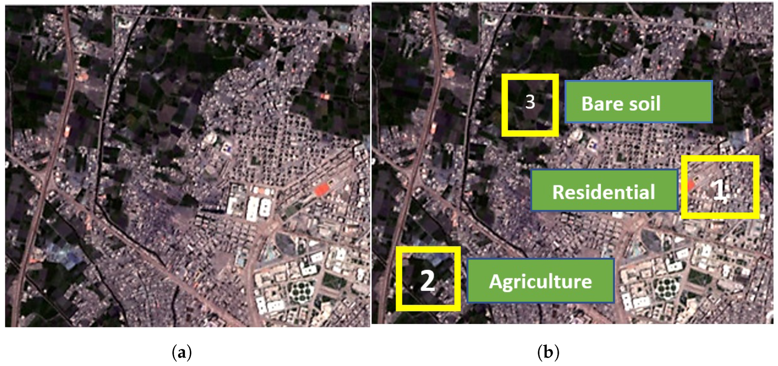
The initial step involved collecting and representing the data, following which a mosaic image was produced from input images that contained multiple bands of data. They are high-resolution images with 4 bands (RGB and near-infrared) generated by re-sampling input images using the k-nearest neighbor $KNN$ approach. In Figure 5a, a mosaic image is generated and then the characteristics of various objects within it are identified and used to classify them according to their shape, color, type, and the land cover they appear on. The resulting data are divided into eight distinct categories, each with detailed descriptions of their sub-categories as listed in Table 1. In this current stage, a fresh set of categories is introduced and a training dataset is generated. The process involves digitizing the detected objects for each class and saving them as a separate category in the vector layer. Subsequently, each category within the training dataset is assigned a distinctive number. As depicted in Figure 5b the numbers 1, 2, and 3 represent three specific types from the defined classes: residential, agriculture, and bare soil. These numbers are used to symbolize different categories, while the shapes depict the corresponding digitized area associated with each type. Finally, a distinct color is assigned to each category, as illustrated in Table 1.

The classifiers used to train and build the proposed LULCRV model are SVM, RF, decision tree (DT), NB, and ANN, which are discussed later in detail. To conduct the classification process, the images fed into the model are divided into a collection of samples, based on the vector layer. A sampling technique is employed for all categories, which is based on the number of samples in the smallest category, referred to as the “number”. This “number” adjusts the number of samples based on the smallest class, which in the case of class 2, is 119. These samples are then split into two equal sets of 50% each for training and testing purposes.

The accuracy of classification is measured using five types of measures that is, precision, recall, f-score, kappa index, and confusion matrix. They are defined and calculated as the true positive (TP) for recognized objects, false negative (FN) for non-detected ones, and false positive (FP) for incorrectly identified ones. The f-score, precision, and recall values range from 0 to 1, where 0 means low identification for a specific class and 1 means ideal identification. Equations (1)–(3) describe precision, recall, and f-score, respectively.

$$Precision=\frac{TP}{TP+FP}$$

(1)

$$Recall=\frac{TP}{TP+FN}$$

(2)

$$f-score=2\times \frac{precision\times recall}{precision+recall}$$

(3)

4.1.1. Heuristic Models

SVM is a machine learning technique that has been employed in LULC classification. The SVM algorithm identifies a hyperplane that maximizes the separation between the various classes in the data based on the attributes or features of the data. The SVM algorithm is well suited for LULC classification tasks due to its ability to manage complex, non-linear relationships between the features and classes [23]. It can also accommodate large datasets with numerous attributes or features. Moreover, SVM is robust when handling noisy data, which makes it a valuable tool in LULC classification scenarios where the input imagery may be prone to noise or inaccuracies. The SVM formula can be written as follows:

$$\begin{array}{c}\hfill Maximize\sum _{i=1}^n{\alpha }_i-\frac{1}{2}\sum _{i,j=1}^n{\alpha }_i{\alpha }_j{y}_i{y}_j.K(x_i,x_j)\\ \hfill Subjectto:\sum _{i=1}^n{\alpha }_i{y}_i,0\le {\alpha }_i\le C\end{array}$$

(4)

Coefficients (${\alpha }_j$) in the model are constrained to be non-negative, and any data point $x_i$ that corresponds to an ${\alpha }_j$ value greater than zero is considered a support vector. The parameter C is used to balance training accuracy and model complexity, allowing for superior generalization capabilities. Additionally, a kernel function K is employed to transform the data into a higher-dimensional feature space, enabling linear separation.

SVM employs two cost parameters: C and Nu. C is utilized to balance the maximization of the margin of the decision function with the accurate classification of training examples. If the decision function can correctly classify all training points, a smaller margin will be tolerated for higher values of C. Conversely, a lower value of C will produce a wider margin at the expense of training precision. Essentially, C acts as a regularization parameter in the SVM. The parameter “Nu” sets an upper limit on the fraction of margin error and a lower limit on the fraction of support vectors relative to the total number of training examples. For example, if Nu is set to 0.05, the SVM algorithm will ensure that no more than 5% of the training examples are misclassified, although this may result in a smaller margin. Additionally, the algorithm will ensure that the number of support vectors is at least 5% of the total training examples [23].

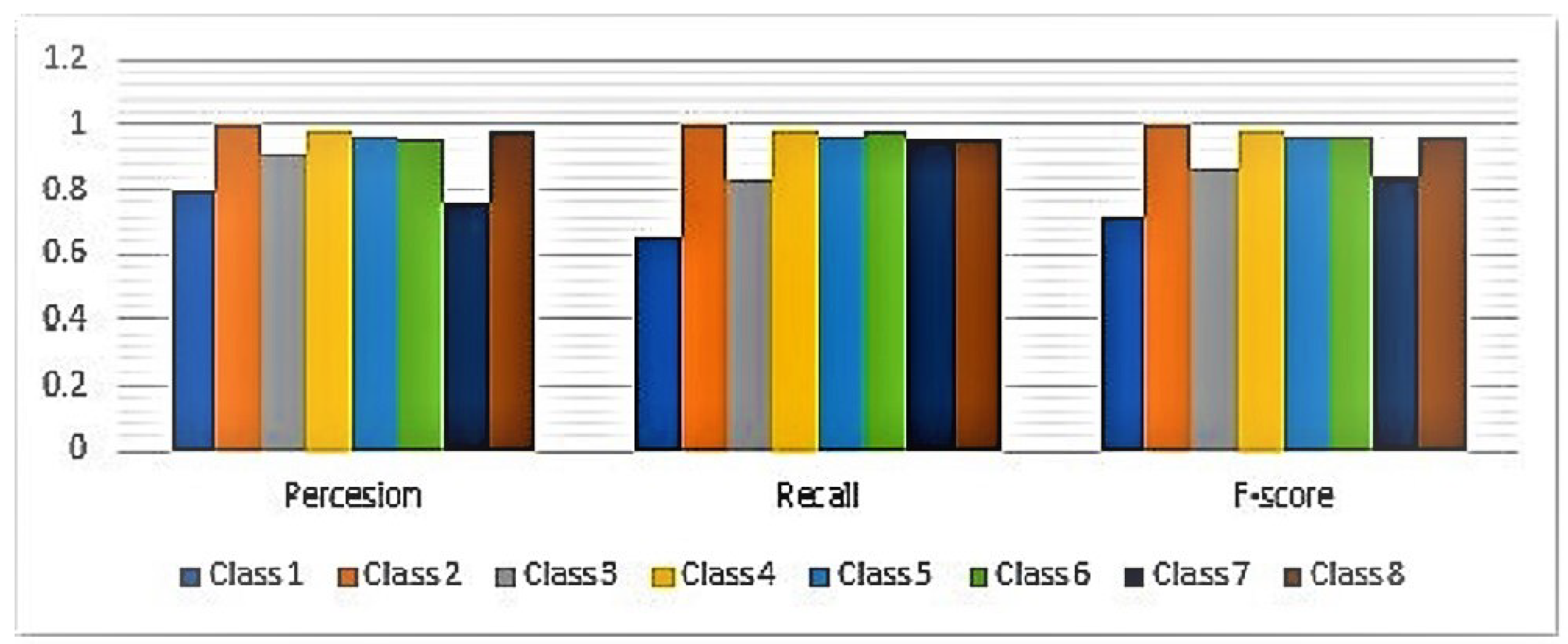
The precision, recall, and f-score values obtained from the SVM/confusion matrix are shown in

Table 2. Precision, recall, and f-score values of proposed eight classes using the SVM classifier.

	Class 1	Class 2	Class 3	Class 4	Class 5	Class 6	Class 7	Class 8
Precision	0.795918	1	0.907407	0.983051	0.966102	0.95082	0.756757	0.982456
Recall	0.661017	1	0.830508	0.983051	0.966102	0.983051	0.949153	0.949153
F-score	0.722222	1	0.867257	0.983051	0.966102	0.966667	0.842105	0.965517

. In summary, class 7has the lowest precision of 0.75; class 1 has the lowest recall and f-score values of 0.66 and 0.72, respectively; class 2 has the highest precision, recall, and f-score values of 1; and class 4 has values of 0.98, as shown in Figure 6.

Random Forest is a type of machine learning algorithm that is capable of performing classification and regression tasks. RF has demonstrated considerable success in LULC mapping tasks, which involve identifying and categorizing various types of LULC present within a given geographic area [24]. The RF algorithm constructs a forest of decision trees using a training set X = x1, x2, …, xn, with Features F = f1, f2, f3, …, fm. A new training set of size N is formed by selecting subsets from the original set with replacement, where each subset is created by randomly choosing N samples with a set of features Y, while Y is the number of features in new samples and Y ≤ M. As a result, some samples may be repeated in the new set while others may be absent [25,26,27].

The precision, recall, and f-score values obtained from the RF classifier/confusion matrix are shown in

Table 3. Precision, recall, and f-score values of proposed eight classes using RF classifier.

	Class 1	Class 2	Class 3	Class 4	Class 5	Class 6	Class 7	Class 8
Precision	0.666667	1	0.9	0.966667	0.907692	0.982143	0.726027	0.961538
Recall	0.644068	1	0.762712	0.983051	1	0.932203	0.898305	0.847458
F-score	0.655172	1	0.825688	0.97479	0.951613	0.956522	0.80303	0.900901

. Class 1 has the lowest and class 2 the highest of all these measures, followed by classes 4, 5, and 6, as shown in Table 3 and Figure 7.

DT is a type of machine learning algorithm that can be used for classification and regression tasks. There are several parameters that you can adjust when using decision trees for LULC classification, such as the depth of the tree, the splitting criterion, and the minimum number of samples required to split a node [28]. The DT method can be expressed as follows: given a dataset D = (x1, y1), (x2, y2), …, (xn, yn), where xi represents the features of the ith sample and yi is the corresponding label, a tree T is split based on the selected feature value(s) to create child nodes for each subset. This process is repeated recursively for each child node until a stopping criterion is met, such as reaching a maximum tree depth, having a minimum number of samples per node, or achieving a certain level of homogeneity/impurity.

Table 4. Input values of parameters in DT and RF classifiers.

Parameters	Maximum Depth of Tree	No. of Samples before Splitting
RF	(10 to 30)	10
DT	(5 to 30)	10

shows the default values of parameters for RF and DT [27,29]. As shown in Table 4, we set the maximum depth of tree in RF and DT up to 30 to simplify the tree and improve its generalization performance. The optimal value for parameters of DT and RF depends on the specific dataset and problem being solved, and can be determined through hyperparameter tuning.

As shown in

Table 5. Precision, recall, and f-score of proposed eight classes using DT classifier.

	Class 1	Class 2	Class 3	Class 4	Class 5	Class 6	Class 7	Class 8
Precision	0.727273	0.967213	0.787879	1	0.964912	0.949153	0.806452	0.929825
Recall	0.677966	1	0.881356	0.932203	0.932203	0.949153	0.847458	0.898305
F-score	0.701754	0.983333	0.832	0.964912	0.948276	0.949153	0.826446	0.913793

, the most reliable prediction is for a large number of class 2 samples and the worst are the class 1 predictions of 0.727273, 0.677966, and 0.701754 for precision, recall, and f-score, respectively. Samples belonging to class 2 were accurately predicted across the board while the prediction accuracy for class 1 was the lowest. Thus, for class 2, the precision, recall, and f-score are 0.967213, 1, and 0.983333, respectively. This implies that the greatest interference is performed between class 1 and the others and, according to the DT algorithm, class 2 is segregated with non-interference. In Figure 8, graphs of the precision, recall, and f-score classes with high vs. lower ratings are illustrated.

NB is a machine learning algorithm that assumes the input features are independent and have a Gaussian distribution. It is often used for classification tasks, such as LULC mapping, where the goal is to classify different types of LULC based on a set of input features [30]. By training on labeled data, NB can learn the relationship between these input features and the corresponding LULC classes, allowing it to accurately predict the class of new, unlabeled data. NB can be expressed as

$$y=argma{x}_{y}P\left(y\right)\coprod _{i1}^{n}P\left(xi\right|y)$$

(5)

where variable y is the class variable X that represents the parameters/features and P(Y) the classifier with maximum probability.

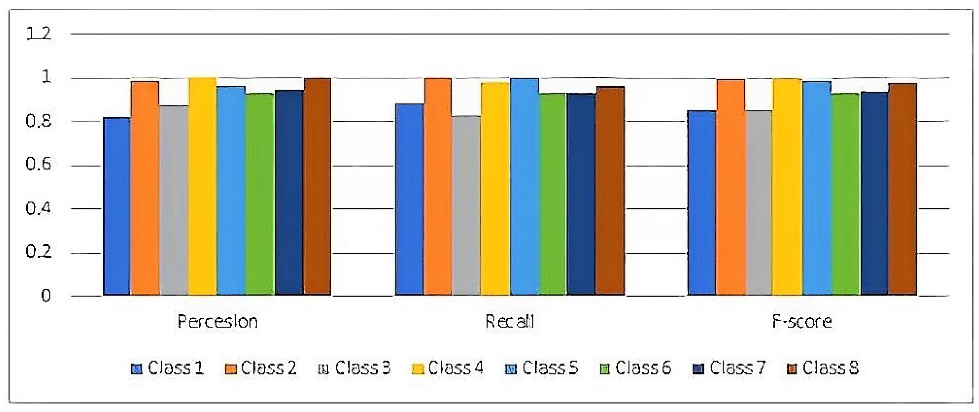
The precision, recall, and f-score values obtained from the NB classifier/confusion matrix are shown in

Table 6. Precision, recall, and f-score values of proposed eight classes using NB classifier.

	Class 1	Class 2	Class 3	Class 4	Class 5	Class 6	Class 7	Class 8
Precision	0.825397	0.983333	0.875	1	0.967213	0.932203	0.948276	1
Recall	0.881356	1	0.830508	0.983051	1	0.932203	0.932203	0.966102
F-score	0.852459	0.991597	0.852174	0.991453	0.983333	0.932203	0.940171	0.982759

. The lowest ones are for classes 1 and 3, and the highest for classes 2, 4, 5, 8, 6, and 7. These values are mapped in Figure 9.

4.1.2. Artificial Neural Networks

We applied Artificial Neural Networks (ANNs), which are a broad class of machine learning models that can be used for LULC classification. Here is a general equation that describes the forward pass of a feedforward ANN:

$$Y=f(W_2\times f(W_1\times x+b_1)+b_2$$

(6)

The model’s specifications include training with 1000 iterations, 5 nodes in the hidden layer, and classifications into 8 distinct classes. In Equation (6), x is the input, Y is the output (a vector with 8 elements, one for each land cover class), $W_1$ is the weight matrix for the input layer (with dimensions 5 $\times n$, where n represents the total number of input features included in the model), $W_2$ is the weight matrix for the output layer (with dimensions 8 × 5), $b_1$ is the bias vector for the input layer (with length 5), and $b_2$ is the bias vector for the output layer (with length 8) [26,27]. The activation function f used in the hidden layer is the hyperbolic tangent function (tanh) Equation (7):

$$tanh\left(x\right)=(e^x-e^{(-x)})/(e^x+e^{(-x)})$$

(7)

The softmax function is applied to the output layer as the activation function [31,32] which normalizes the outputs of the network so that they sum to 1 and represent a probability distribution over the 8 classes, as in Equation (8):

$$y_i=\frac{e^{z_i}}{{\displaystyle \sum _{j=1}^8}{e}^{z_j}}$$

(8)

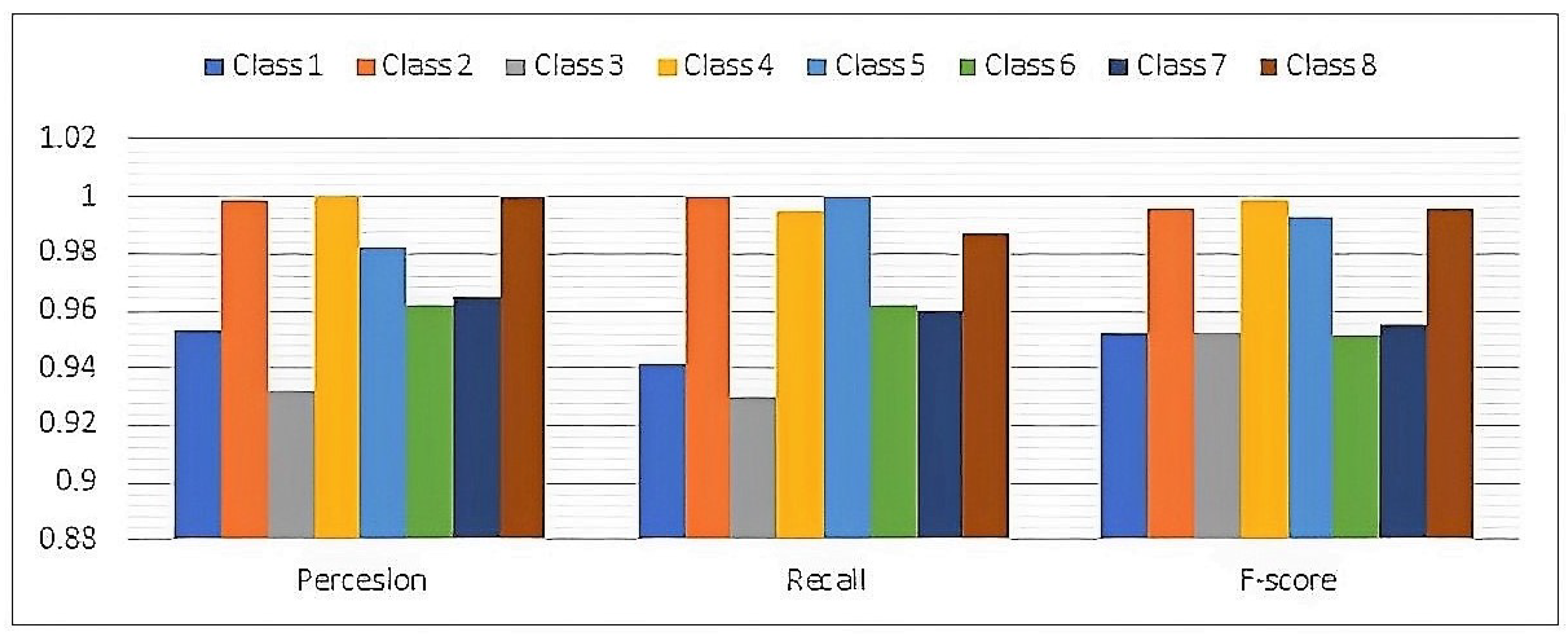
The precision, recall, and f-score values obtained from ANN classifier/confusion matrix are shown in

Table 7. Precision, recall, and f-score values of proposed eight classes using ANN classifier.

	Class 1	Class 2	Class 3	Class 4	Class 5	Class 6	Class 7	Class 8
Precision	0.953045	0.99890	0.932401	1	0.982130	0.962201	0.965276	1
Recall	0.941356	1	0.930508	0.995061	1	0.962204	0.960203	0.987102
F-score	0.952459	0.995698	0.952174	0.998907	0.99305	0.951304	0.95506	0.995750

. Those for all classes are between 0.92 and 1 which are higher than those of the other classifiers used. These values are shown in Table 7 and Figure 10.

4.2. Prediction

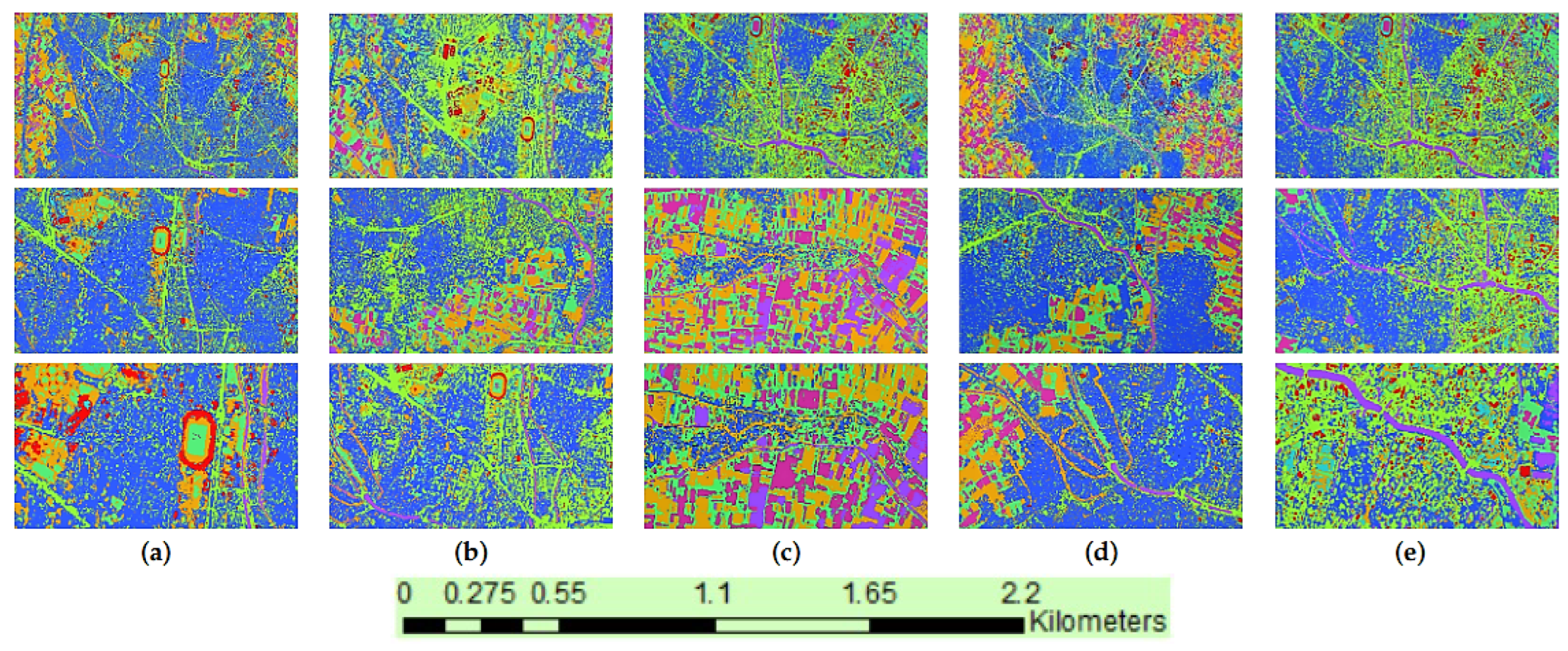
The LULCRV proposed model generates and predicts an LULC map; Figure 11 shows the LULC map generation of the proposed LULCRV. Columns (a), (b), (c), (d), and (e) show the generated LULC maps on different scales from the DT, RF, SVM, NB, and ANN models, respectively.

The average area for each class as it appears on the LULC map that was generated is in

Table 8. The average area for each class as it appears on the LULC map.

	Class 1	Class 2	Class 3	Class 4	Class 5	Class 6	Class 7	Class 8	Total Area
Area	44,638,065	66,286,170	106,047,648	3,753,765	205,717,833	108,261,828	7,976,925	58,521,978	601,204,212

.

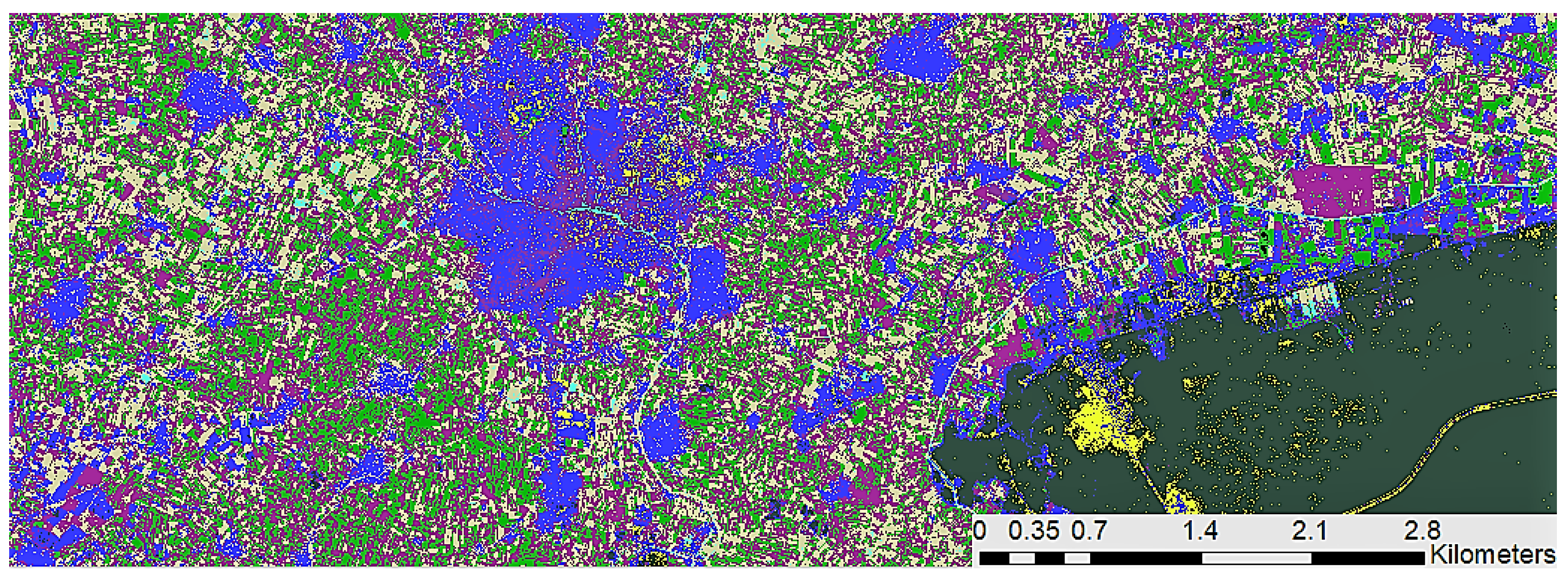
To evaluate the accuracy of an individual map, we compare it with the reference data and determine the level of agreement between them [33]. The reference data in Figure 12 comprises a vector layer created by generating random samples that are unlabeled initially, as in Figure 13. Subsequently, we assign labels to each of these points.

Kappa Index

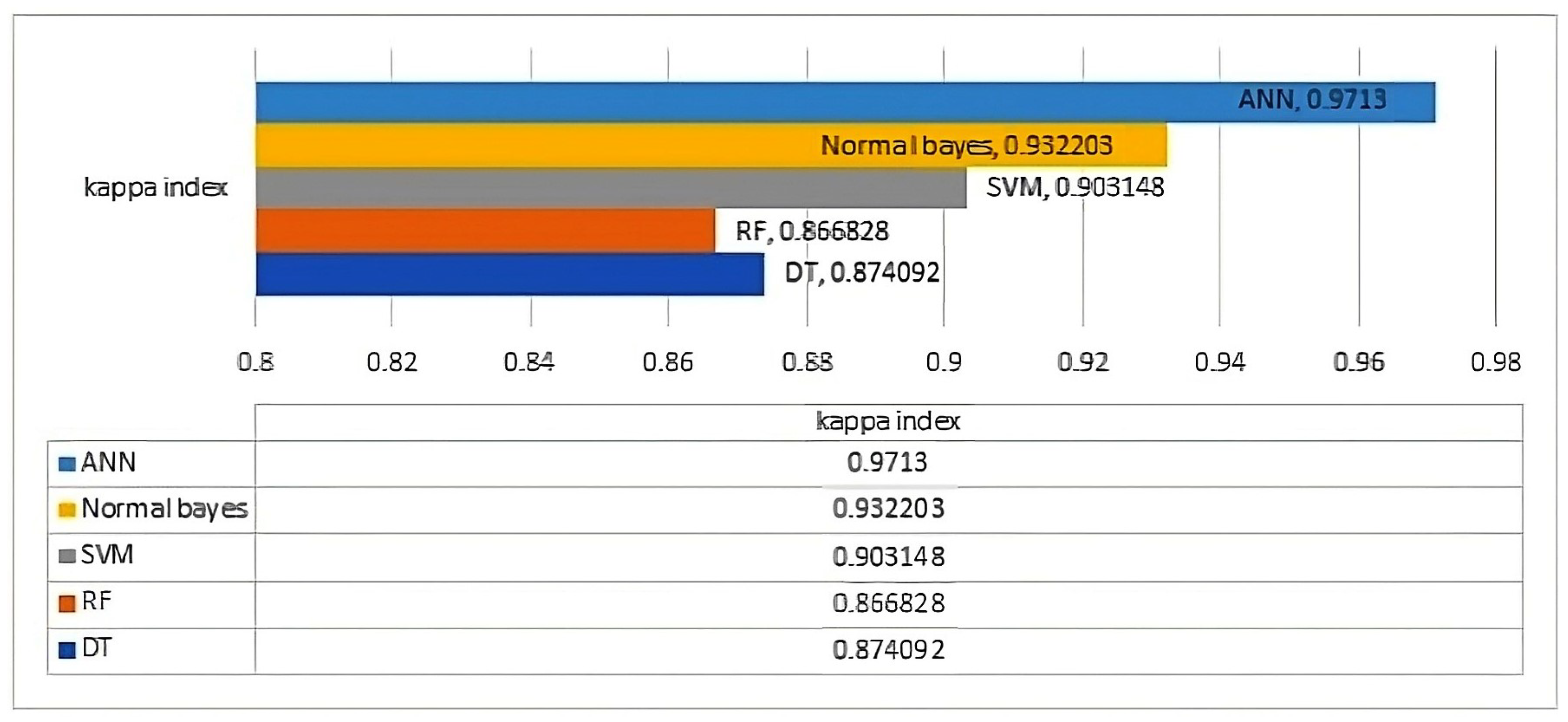
The kappa index is measured for the five models and recorded in Figure 14. Kappa is derived from Cohen’s kappa formula, where the probability of random agreement is subtracted from the probability of agreement, and then the result is divided by 1 minus the probability of random agreement. The higher this index is, the more efficient and identical prediction is. The ANN is the model with the highest kappa index with 0.97130, NB is the second with 0.932203, SVM is the third with 0.903914, while the $RF$ and $DT$ models have lower values.

4.3. Analysis and Discussion

In

Table 9. Summary of results obtained by various classification models.

Model/Summary Results	No. of Full Separated Classes	No. of Classes with the Lowest Interference ⩾ 55	No. of Classes with the Medium Interference (49 to 54)	No. of Classes with the Highest Interference (38 to 48)	No. of Enhanced Classes
$DT$	1	3	3	1	0
$RF$	2	2	2	2	0
SVM	1	5	1	1	0
$NB$	2	4	2	0	1
ANN	2	6	0	0	4

is a summary and comparison of a set of elements that enhance each model. They are defined as the number of fully separated classes with non-interference where all samples are correctly predicted; the number of classes with the lowest interference in which the predicted correct samples are ⩾55 of 59; the number of classes with medium interference in the range of (49 to 54) correct of 59 samples; the number of classes with maximum interference in the range of (38 to 48) correct samples of 59. The number of enhanced classes is the number of classes that transfer into low- or non-interference classes from medium or high ones.

As shown in Table 9 and Figure 15, both NB, and ANN enhance the separation of high-interference classes through higher identifications of objects in the learning process and better prediction of these objects in the classification process, which reduces the number of high-interference classes and transforms them into low-interference ones.

Regarding the LULCRV model, it is observed that classes 1 and 3 (residential and bare soil, respectively) have high interference with class 7 (roads). The reason for this is that there are common features of the objects belonging to these classes in the captured images. Similar features are described by color, band length, and sometimes shape. To solve the problem of interference, the vector layer with color segments is defined, enhanced, and updated for each class.

While ANN classifier/model achieves better performance when applied to all classes than the others, it uses an accurate input that identifies the network’s pattern and pre-processing by re-sampling the KNN algorithm to the input mosaic and obtaining a finer resolution. Furthermore, high-resolution images and two forms of training vector data are used in the training model. The first one is an object-based model that holds the features of objects such as boundaries, colors, and shapes, and the second is pixel-based that is captured randomly from different samples on the generated LULC map to measure its accuracy.

For the NB classifier, its key to success is to correctly predict an incoming test instance using the class of training instances. It does not necessitate a large number of observations for each potential combination of variables, which is especially useful when working with high-dimensional input data, such as a dataset with dimensions of 7939 × 3775 pixels. Additionally, the effect of a variable on a particular class in this classifier is independent of the value of another variable. Although this assumption simplifies the computation, it can occasionally outperform more complex computations.

Its learning iterations are the key explanation for the more powerful separation of classes and estimation of the ANN. Once the number of layers and the number of nodes in each layer are determined, its back-propagation ANNs configuration can be established. Then, the learning task involves assigning appropriate weights to every edge or link to ensure accurate classification of the unlabeled data. The weights and biases are initially allocated randomly in the range of [0, 1] during the back-propagation ANN learning. Then, an instance is added to the network and produces an output based on its current synaptic weights. This output is compared to a known good output, and a mean-square error is computed. The error is then propagated backwards through the network, and the weights of each layer are adjusted. This entire process is repeated with each instance and then returns to the first instance, continuing in a loop. The loop continues until the cumulative error value falls below a predetermined threshold.

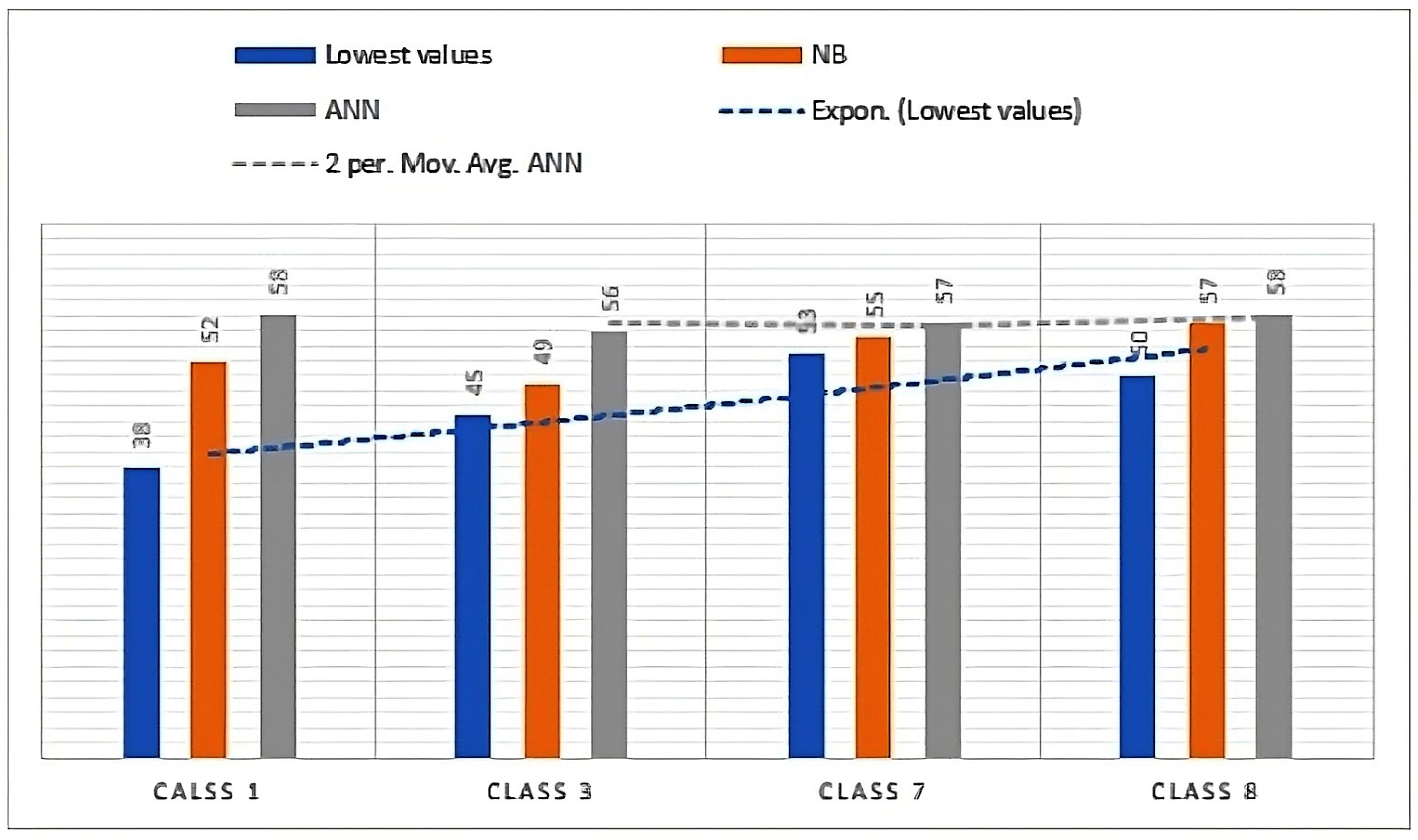
It can be concluded that classes 1 and 3 are transformed from high-interference classes to medium-interference ones by the $NB$ model and from high- to low-interference ones by the ANN model. In Figure 16 the difference and enhancement of the transformed groups are illustrated; for instance, the well-recognized samples are transformed from 38 into 52 by the $NB$ model and 58 by the ANN classifier. Finally, the proposed LULCRV model and previous ones are compared. It is found that Allam, M., in [4] used satellite images with a 30 m spatial resolution to identify changes in LULC patterns in the Fayoum city of Egypt. However, The image classification dataset was limited to four distinct classes, while the proposed LULCRV model is applied with 3.0 m spatial resolution satellite images for the same region. High-resolution images can detect large numbers of objects and their characteristics, which is another consideration in the previous study focused on 6 RGB 3-band images. Furthermore, the proposed one uses 65 4-band images and applied 5 models/classifiers, the $SVM$, $RF$, $DT$, $NB$, and $ANN$ models, while the previous related work used the MLC for classification. Finally, the proposed LULCRV outperforms the related work achieving 98% accuracy against 96%. Krueger, H., in [17] applied $RF$ and SVM classifiers and attained 0.85 as their accuracy and a kappa of 0.81 for $RF$ compared with the proposed RF LULCRV’s 0.86. The main difference is that the SVM and $RF$ were applied to a large data 211 spot. This prevented the use of NNs, including an ANN, which may be more robust to the large size of satellite images, with pictures also captured by 3-band radar. C Marais, S., in [8] developed a WFCNN model that was trained using 6 4-band aerial images and then applied to 587 labeled images for testing. Two versions of the model were tested using Gaofen 6 and aerial images, and their performance was compared against SegNet, U-Net, and RefineNet. The precision, recall, and f1-score values of the WFCNN model were superior to those of the other models, indicating the advantages of performing pixel-by-pixel segmentation. There is little difference between the LULCRV and WFCNN classification models in terms of precision, recall, and f-score values because of the 4-band images and deep neural network used in both. Comparisons of the three elements of dataset, model, and result of the previously mentioned studies and proposed LULCRV model are provided in

Table 10. A comparison between the proposed study and related studies.

Model	Dataset	Results	Paper/Year
Venter, Z.S., Barton, D.N., Chakraborty, T., Simensen, T., Singh, G. 2022 [19]	DW, WC, and ELC	FCNN	Overall accuracy = 89.26%
Mona Allama Noura Bakrb Walid Elbably, 2020 [4]	6 Landsat satellite images and a 30 × 30 m spatial resolution	MLC and NDVI	Overall accuracy = 96%
Chengming Zhang, Yan Chen, Xiaoxia Yang, Shuai Gao, Feng Li, Ailing Kong, Dawei Zu 1, Li Sun, 2020 [9]	GF-6 images	WFCNN	Precision = 91.93% Recall = 94.14% fscore = 0.9271 kappa = 0.8693
C. Marais Sicre, R., Fieuzal, F. Baup, 2019 [8]	Composed of 211 spots	SVM and RFs	Overall accuracy = 0.85 kappa = 0.81
Proposed LULCRV, 2023	65 images with 3.0 spatial resolution	DT and RFs SVM and NB ANN	Precision = 0.9821 Recall = 0.9871 f-score = 0.9622 kappa = 0.971

.

5. Conclusions

In this research, a prediction model for LULC is proposed. It consists of 8 land use/cover classes using 3.0 m spatial multi-spectral high-resolution satellite images. The main objective is to build an ML classification model for land use/cover called LULCRV. It learns on high-resolution multi-spectral images and vector data; the raster image holds band information of specific pixels while the vector layer contains the definition of classes along with the corresponding class number. LULCRV involves pre-processing, labeling, model building, and prediction phases. During the pre-processing phase, the input data are prepared for the proposed LULCRV model, holding a vector training set and raster mosaic images. In the labeling phase, objects are extracted from input images based on their features, colors, shapes, and boundaries, and then assigned a class number and stored in a vector layer, as these objects. The model building phase builds the proposed LULCRV model using a set of classifier models, that is, $SVM$, $RF$, $NB$, $DT$, and $ANN$. The prediction phase generates an LULC map for the entire satellite image. The performance of the model is measured using metrics of precision, recall, f-score, and kappa index ratings. It is observed that the ANN achieves higher accuracy measures than the others.