Attention Mechanism-Combined LSTM for Grain Yield Prediction in China Using Multi-Source Satellite Imagery

Abstract

Grain yield prediction affects policy making in various aspects such as agricultural production planning, food security assurance, and adjustment of foreign trade. Accurately predicting grain yield is of great significance in ensuring global food security. This paper is based on the MODIS remote sensing image data products from 2010 to 2020, and adds band information such as vegetation index and temperature to form composite remote sensing data as a dataset. Aiming at the lack of models for large-scale forecasting and the need for human intervention in traditional models, this paper proposes a grain production estimation model based on deep learning. First, image cropping and yield mapping techniques are used to process the data to generate training samples. Then the channel and spatial attention mechanism (convolutional block attention module, CBAM) is added to extract spatial information in different remote sensing bands to improve the efficiency of the model. Long short-term memory (LSTM) neural networks are added to obtain feature information in the time dimension. Finally, a national-scale grain yield prediction model is constructed. After the study, it was found that the LSTM model using a combination of multi-source satellite images and an attention mechanism can effectively predict grain yield in China. Furthermore, the proposed model was tested on data from 2018 to 2020 showing an average ${\mathrm{R}}^2$ of 0.940 and an average RMSE of 80,020 tons, indicating that it can predict Chinese grain yield better. The model proposed in this paper extracts grain yield information directly from the composite remote sensing data, and solves the problem of small-scale research and imprecise yield prediction in an end-to-end manner.

1. Introduction

In recent years, floods, wind and hail, geological and other natural disasters have occurred many times around the world, and droughts, earthquakes and low-temperature freezes have also occurred to varying degrees. Various natural disasters have caused certain impacts on agricultural production in some areas, resulting in reduced food crop production, and the issue of food security has become a hot topic of concern. At the same time, global environmental climate change and international conflicts have threaten food security [1,2]. To address food security issues, FAO promotes global food security and improved food supply by promoting efficient agricultural technologies, providing knowledge on food nutrition, supporting rural economic development and raising farmers’ incomes. In addition, FAO is committed to promoting fairness and transparency in global food trade to ensure the stability and sustainability of global food markets.

Agriculture plays a crucial role in modern society, and the growing global population further highlights the importance of food security [3]. The primary solution to the food security issue is to accurately predict grain yield. Accurately predicting grain yield in advance to obtain first-hand quantitative data will not only effectively improve our grain production process and trade, but also inform policy makers of potential food shortages, price volatility and trade imbalances. Investors use yield predictions to determine the profitability of agricultural investments, which can affect the overall economic growth of a region or country. Farmers rely on yield predictions to effectively plan their planting and harvest schedules, as well as manage their crop inputs and resources.

Current grain yield prediction methods have several limitations that limit prediction accuracy. First, yield prediction models are usually based on a single piece of historical data. Most studies assess the impact of climate change on agricultural production based on specific regions and do not consider the impact of human economic behaviour [4]. Second, the accuracy of yield prediction models may be affected by data quality and availability, and different data may produce different predictions. Third, yield prediction models usually do not take into account the complex interactions between certain factors and crop growth, including soil conditions, rainfall, temperature, solar radiation, and human activities.

Traditional models often use statistical models and plant growth models for yield prediction, which can be effective in predicting grain yield to a certain extent. However, grain yield is often affected by the spatial distribution and temporal variation of the growing environment, and traditional models lack spatial and temporal information of plant growth, which leads to poor prediction accuracy and lack of robustness [5]. At the same time, traditional methods require field surveys, resulting in high time consumption and material costs [6], and can lead to problems of small yield estimation areas and poor timeliness. In contrast, with the development of technology, remote sensing technology is widely used for grain yield prediction due to its advantages of good timeliness and low cost, and its ability to effectively cope with the problems of complex terrain, scattered cultivated land and diverse crops [7]. Therefore, some researchers have combined remote sensing data and meteorological data to establish grain yield prediction models [8], while some studies have combined remote sensing data with plant growth models for yield prediction [9,10], and these studies have demonstrated that models using remote sensing technology can be an appropriate solution to the previous problems of difficult data statistics, high labour consumption and low accuracy. Furthermore, since remote sensing images have spatial information, the use of these data can be effective in making more accurate predictions using spatiotemporal information [11], and it has been shown [12] that the use of traditional models is laborious, error-prone, costly, and inefficient in the study of maize yield prediction in Africa. Tuvdendorj et al. [13] chose to use NDWI, VSDI, and NDVI to develop regression prediction yield models for spring wheat yields in Selenge and Darkhan Provinces of Mongolia. The study conducted by Tuvdendorj et al. involved a rigorous data processing methodology to analyse the plant growth level in a particular area. The raw MODIS data was subjected to conventional techniques such as re-projection, mosaic, and cropping. The researchers then extracted the relevant bands and calculated indices, such as NDVI and NDWI, to represent the plant growth level. Finally, a regression prediction model was built by combining the NDVI and NDWI indices to accurately predict the plant growth level. As a comparison, the direct use of remote sensing images to predict grain yield is a more cost-effective option.

With the development of computer technology, a large number of studies have started to use machine learning methods to build models due to its advantage of being able to handle complex agricultural data. Some researchers have used machine learning to build a low-cost grain yield prediction model [14] and found that it can effectively improve the prediction efficiency. Yang et al. [15] used multispectral remote sensing data collected by an unmanned aerial vehicle (UAV) in a major rice growing region in southern China and applied a neural network model to predict rice yield, achieving superior results compared to traditional regression models. Meroni et al. [16] used small data samples to train neural networks to predict grain yield, and Paudel et al. [17] combined agronomic principles with machine learning to build a large-scale grain yield prediction model using a modular approach so that the model could be used for different crop yield prediction in different countries, and demonstrated experimentally that the performance of the machine learning model would be better with the addition of new data sources. Using science, technology and knowledge and experience to achieve rational use and planning of resources can meet people’s survival needs and reduce the waste of resources to achieve sustainable development of resources.

However, most of the existing data are used for single crop yield prediction at the county or municipal scale using normalized difference vegetation index (NDVI), enhanced vegetation index (EVI), etc., [18], lacking multiple sources of data and holistic prediction of multiple crops. Furthermore, we also note that the existing machine learning methods usually process the relevant indices (e.g., NDVI, EVI, etc.) of a region after averaging [19] or sampling [20] (selecting the maximum or minimum values) and then using them as input data for the model, neglecting the study of subtle features. Therefore, in order to improve the prediction of grain yield, this paper proposes the use of hybrid neural networks for prediction of composite data. The contribution of this paper is as follows.

• A multi-source dataset was created containing grain yield and remote sensing images, temperature and vegetation index with spatial and temporal information.
• Using the cropping and mapping method, the remote sensing image of each province is cropped into $128\times 128$ size image blocks, and the yield weights of each block are calculated and mapped through the land-use classification mask, effectively combining multiple information for large-scale prediction.
• The incorporation of spatial and channel attention mechanisms with LSTM neural networks is proposed to learn the trend characteristics of different categories of plant indices and indices in crop growth in composite data as a way to improve the accuracy of model predictions.

2. Materials

2.1. Study Area and Data Acquisition

The study area selected for this paper is the People’s Republic of China, and the data collection comes from 31 provincial administrative regions. China can be divided into four geographical regions based on geographic and humanistic natural characteristics, namely the Southern Region, the Northern Region, the Northwest Region, and the Qinghai–Tibet Region. The northern region includes the Northeast Plain, the North China Plain, and the Guanzhong Plain, all of which are important agricultural production areas in China. Because of the climate, the main food crops north of the Great Wall are spring wheat, maize, sorghum, soybeans and potatoes, while south of the Great Wall, winter wheat, corn and rice can be grown. The southern region has abundant heat and precipitation, and has very good conditions for agricultural production. The Chengdu Plain and the middle and lower reaches of the Yangtze River are both major grain-producing regions in China. The Northwest and Qinghai–Tibet Region can only grow some cold and drought-resistant crops due to scarce precipitation and high altitude and cold climate, respectively, but the yield is not high.

The acquired remote sensing image data were obtained from NASA’s Earth Science Data and Information System (ESDIS), among which the data products used were MOD11A2, MOD13A1 and MOD15A2H, and the detailed information is shown in

Table 1. MODIS data products and band information.

Product Name	Band	Time Resolution	Spatial Resolution	Valid Range
MOD11A2	Daytime Land Surface Temperature	8 Days	1 km	7500–65,535
	Nighttime Land Surface Temperature
MOD13A1	Normalized Difference Vegetation Index	16 Days	0.5 km	−2000–10,000
	Enhanced Vegetation Index
MOD15A2H	Leaf Area Index	8 Days	0.5 km	0–100
	Fraction of Photosynthetically Active Radiation

. The data are chosen to span the period from 2010 to 2020, a total of 11 years.

Among them, the land-use classification information of China was selected from the Resource Environment Science and Data Center, Institute of Geographical Sciences and Resources, Chinese Academy of Sciences.

In addition, the grain crop production data for the study area are obtained from the China Statistical Yearbook [21] for 2011–2021 (China Statistical Yearbook data lagged by one year). The grain crop production data include three cereal crops: rice, wheat, and maize, in addition to beans and potatoes. These crops have different growth cycles and harvesting times are scattered among different months, so our training sample contains monthly data in order to improve the predictive performance of the model.

2.2. Data Processing

Depending on the study area and time, we selected data from the sinusoidal tile grid of the MODIS product (Figure 1). Because the data provided by MODIS is not uniform in resolution for time or space, we used the GDAL library for batch processing while using ArcGIS software (v10.8.2). First, we extracted the data layers we needed from the downloaded raw files in HDF format and saved them as raster files in TIF format. The scattered rasters that have undergone the mosaic operation are also combined, and the MOD11A2 data are individually resampled to a spatial resolution of 500 m so that all data have the same resolution. Then all images were uniformly reprojected onto the China Geodetic Coordinate System 2000 to facilitate subsequent experiments. Next, we processed the data according to the valid range and scale factor provided by ESDIS. Finally, all data were cropped according to the provincial administrative divisions of China, and all data were synthesized on a monthly basis at a temporal resolution (Figure 2) to make the time series consistent. In order to reduce useless information interference and increase effective data density, we used land-use classification masks to extract data on the location of farmland distribution. Note that all data are normalized by min–max normalization.

2.3. Grain Yield Prediction Dataset

China has a diverse range of climatic conditions due to its large size and varied topography. Generally speaking, China’s climate can be divided into four main types: continental, monsoon, subtropical, and highland. Each of these climate types has different impacts on crop yields in different areas of the country. In areas with a continental climate, which are mainly located in the northern part of China, the climate is characterized by large temperature fluctuations between seasons and low precipitation. This type of climate is generally not suitable for high-yield agriculture, and crops such as wheat and corn are the main crops grown in these areas. In areas with a monsoon climate, which are mainly located in southern China, the climate is characterized by high temperatures, high humidity, and heavy rainfall in the summer months. This type of climate is suitable for the cultivation of rice, which is the main crop grown in these areas. In areas with a subtropical climate, mainly located in the southeastern part of China, the climate is characterized by mild winters, hot summers, and abundant rainfall throughout the year. This type of climate is suitable for the cultivation of crops such as tea, citrus fruits, and sugarcane. In areas with a highland climate, mainly located in the southwestern part of China, the climate is characterized by high altitude, low temperatures, and low precipitation. This type of climate is suitable for the cultivation of crops such as barley, potatoes, and wheat. In order to enable the model to better learn the relational features among them, we use the image cropping method to ensure the resolution of each map is of the same size. We cropped the remote sensing image of each province into $128\times 128$ size image blocks, and used the fill 0 value for the image boundary that cannot be completely cropped.

The total grain production of each province in each year was queried from the China Statistical Yearbook, and we used a case-by-case calculation method to map the total production to each image block. First, the land-use classification masks were used as the total area of farmland. The percentage of farmland area in each plot relative to the total farmland area in the corresponding province is then calculated as the production weight of the current image block. Finally, the production of the corresponding image block is calculated based on the calculated weights:

$$X_i=\frac{s_i}{S}\times O$$

(1)

where $X_i$ represents the yield corresponding to each image block, S represents the total farmland area, $s_i$ represents the area of farmland in each image block, and O represents the total yield.

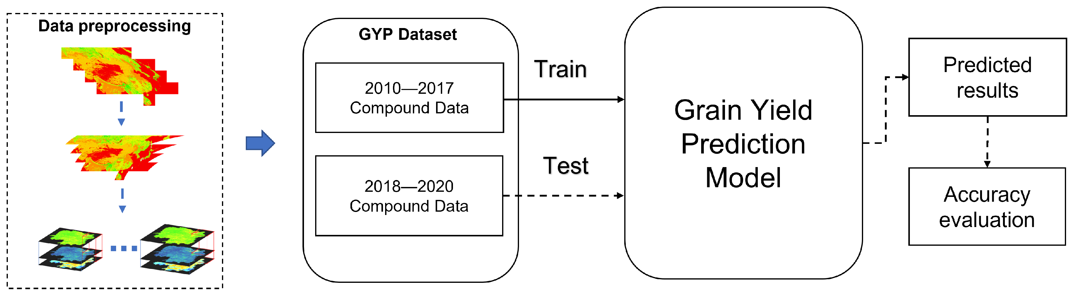
We cropped all the remote sensing images of different bands to the same size, and then fused the six bands of data together, with each band as an image channel. In the time dimension, since the remote sensing images have been previously synthesized to a monthly resolution, we synthesized the remote sensing images together for every 12 months. Finally, a matrix was combined as one of the samples, the shape of which is $(T,C,H,W)$.

Since cropping the images produces many pure black images (all values are 0), after removing these images, a total of 22,303 valid images were obtained. Among them, 16,219 images from 2010 to 2017 were used as the training set and 6084 from 2018 to 2020 were used as the test set. The final grain yield dataset was generated and named as GYP.

3. Methods

3.1. Overall Flow of the Model

Prediction has been a more complex matter due to the number of factors that affect grain yield. Therefore, this paper uses a model of deep learning to perform grain prediction. The model uses convolutional neural networks (CNN) as the basic structure, and then incorporates spatial and channel attention mechanisms to extract features effectively and autonomously. Furthermore, we incorporate a LSTM network to enhance the sensitivity of the model to the temporal features of grain yield. After the data processing in Section 2.2, we used the composite remote sensing data from 2010 to 2017 as the training sample, using 2018–2020 data as a test sample to generate the grain yield prediction model. Finally, the predicted results of the model were compared with the true yield and the model performance is evaluated (Figure 3).

3.2. CNN-LSTM Model with Embedded Attention Mechanism Module

The proposed model in this paper is based on CNN, while introducing an attention mechanism combined with a recurrent neural network (RNN) to form a hybrid neural network model. The overall network structure is shown in Figure 4. Our neural network input layer is designed as a matrix of $(B,12,6,128,128)$ based on our samples, where B represents the batch size, 12 represents the time series, 6 represents the band, and 128 is the height and width, respectively. Before going through the CNN layers, we reshape the matrix to the shape of $(B\times 12,6,128,128)$. After this we add three layers of convolution operation and an average pooling operation. The number of convolutional kernels in the convolutional layer is 12, 8 and 4, respectively, and the convolutional kernel size is $3\times 3$ with a step size of 1. Each convolutional layer is followed by an average pooling layer with a kernel size of $3\times 3$ and a step size of 2. A LeakyReLU function activation operation is also performed after each convolutional layer. We add a convolutional block attention module (CBAM) after the first and third convolutional layers, respectively. This is followed by the LSTM layer with 128 hidden nodes in each layer. Finally, a fully connected layer and an additional dropout layer is used in the fully connected layer.

3.2.1. Attention Mechanism Module

The attention mechanism is a technique used in artificial neural networks to allow the model to selectively focus on certain input features or patterns while processing data. This can be useful in situations where the input data is complex or large, and the model needs to identify important patterns or features that are relevant to the task at hand.

In recent years, in order to further expand the differences between features, research scholars have introduced attention mechanisms into some deep learning models [22,23]. The attention mechanism highlights more representative features by assigning different weighting coefficients, similar to the brain signal processing mechanism specific to human vision, and can be used to obtain target areas that need to be focused on by quickly scanning the entire image [24,25,26,27]. Therefore, to effectively acquire data in composite images, we used CBAM proposed by Woo et al. [28], which combines channel and spatial attention in a lightweight way to embed into the model for feature extraction. The CBAM embedding method is shown in Figure 5.

The overall structure of channel attention is shown in Figure 6. The input data are processed by max pooling and average pooling, and then sent to multilayer perceptron (MLP) for calculation to obtain the transformation results. Then the two sets of channel features obtained after the transformation are included in the element-wise addition operation, and finally the $M_c\left(F\right)$ is obtained by activation with sigmoid function, and its formula is shown in Equation (2). When $M_c$ is calculated using channel attention, the $M_c$ obtained from channel attention is included in the element-wise multiplication operation with the original input feature map F before sending it to spatial attention to obtain $F^{\prime }$, as shown in Equation (3).

$$\begin{array}{cc}\hfill {\mathbf{M}}_{\mathbf{c}}\left(\mathbf{F}\right)& =\sigma \left(MLP\right(AvgPool\left(F\right))+MLP(MaxPool\left(F\right)\left)\right)\hfill \\ & =\sigma (W_1\left(W_0\left(F_{avg}^C\right)\right)+W_1\left(W_0\left(F_{max}^C\right)\right))\hfill \end{array}$$

(2)

where $\sigma$ denotes the sigmoid function, $W_0\in R^{(C/r\times C)}$, and $W_1\in R^{(C\times C/r)}$. Note that the MLP weights, $W_0$ and $W_1$, are shared for both inputs and the ReLU activation function is followed by $W_0$.

After the channel attention is calculated, the spatial attention mechanism (Figure 7) first performs the max pooling and average pooling operations on the input $F^{\prime }$ according to the channel, and then the obtained feature map will be subjected to the concatenation operation on the channel. After completing the channel concatenation, a $7\times 7$ convolution is performed to reduce the dimensionality. Finally, $M_s\left(F\right)$ is obtained by using the sigmoid activation function, and the calculation formula is shown in Equation (4).

$${\mathbf{F}}^{\mathbf{\prime }}=M_c\left(F\right)\otimes F$$

(3)

where ⊗ denotes element-wise multiplication.

$$\begin{array}{c}\hfill \begin{array}{cc}\hfill {\mathbf{M}}_{\mathbf{s}}\left(\mathbf{F}\right)& =\sigma \left(f^{7\times 7}\left([AvgPool\left(F\right),MaxPool\left(F\right)]\right)\right)\hfill \\ \hfill & =\sigma \left(f^{7\times 7}\left([F_{avg}^s;F_{max}^s]\right)\right)\hfill \end{array}\end{array}$$

(4)

where $\sigma$ denotes the sigmoid function and $f^{7\times 7}$ represents a convolution operation with a filter size of $7\times 7$.

Finally, Equations (3) and (4) are used to obtain the final feature map $F^{″}$:

$${\mathbf{F}}^{\mathbf{″}}=M_s\left(F^{\prime }\right)\otimes F^{\prime }$$

(5)

where ⊗ denotes element-wise multiplication.

In the grain yield prediction model, the attention mechanism is used to extract spatial information from different remote sensing bands in order to make more accurate predictions. The attention mechanism is implemented by adding additional layers to the neural network model, trained to learn to focus on relevant features in the input data. The attention mechanism can improve the performance of the model by helping it to better capture and utilize relevant patterns or features in the data, leading to more accurate predictions.

3.2.2. Long Short-Term Memory

The LSTM network is a RNN first proposed in 1997 by Hochreiter et al. [29]. The RNN cannot learn relevant information about the input data when the input gap is large and cannot handle very long input sequences, while LSTM can deal with long-term dependencies by introducing gate functions in the cell structure [30,31], such as the effect of changing processes of grain crops on yield throughout the growth cycle. Therefore, to better obtain the features in the temporal dimension, the LSTM network is introduced.

The cell structure of the LSTM network is shown in Figure 8. Compared with the previous RNN, LSTM adds the concept of the cell state, consisting of three gates: the forget gate, input gate and output gate. They use per-element multiplication between them to control how much of past memory is retained. In this paper, monthly crop changes were used as the time dimension, and 12 months of data were input into the LSTM as a way to extract the effect of crop growth processes on yield.

Among them, the forget gate is calculated as shown in Equation (6), mainly used to decide the retention or forgetting of information. The hidden information $h_{t-1}$ of the previous layer and the input information $x_t$ of the current layer will be sent into the sigmoid function for processing at the same time. The processing result will be between $\left[0,1\right]$. The closer it is to 1, the more it should be retained, and vice versa.

$${\mathbf{f}}_{\mathbf{t}}=\sigma \left(W_f·\left[h_{t-1},x_t\right]+b_f\right)$$

(6)

Furthermore, the equation of the input gate is shown in Equations (7) and (8), mainly used to update the information of the current layer. The hidden information $h_{t-1}$ of the previous layer and the input information $x_t$ of the current layer will be sent into the sigmoid function for processing at the same time. The processing result will be between $\left[0,1\right]$. The closer it is to 1, the more important it will be. Next, the information from the hidden state of the previous layer and the current input is also passed into the tanh function to create a new candidate vector. Finally, the output value of the sigmoid function is multiplied by the output value of tanh. The output value of the sigmoid function will determine which information in the output value of tanh is important and needs to be retained.

$${\mathbf{i}}_{\mathbf{t}}=\sigma \left(W_f·\left[h_{t-1},x_t\right]+b_i\right)$$

(7)

$${\tilde{\mathbf{C}}}_{\mathbf{t}}=tanh\left(W_C·\left[h_{t-1},x_t\right]+b_C\right)$$

(8)

The output gate, shown in Equations (9)–(11), is used to determine the value of the next hidden state, which contains the previously inputted information. The hidden information $h_{t-1}$ from the previous layer and the information $x_t$ from the current layer input are simultaneously sent to the sigmoid function for processing. Then the newly obtained cell state is sent to the tanh function. Finally, the output of tanh is multiplied with the output of the sigmoid function to determine the information that the hidden state should contain. The hidden state is then used as the output of the current cell, and the new cell state and new hidden state are sent to the next time step.

$${\mathbf{C}}_{\mathbf{t}}=f_t\ast C_{t-1}+i_t\ast \widetilde{C_t}$$

(9)

$${\mathbf{O}}_{\mathbf{t}}=\sigma \left(W_o·\left[h_{t-1},x_t\right]+b_o\right)$$

(10)

$${\mathbf{h}}_{\mathbf{t}}=O_t\ast tanh\left(C_t\right)$$

(11)

3.2.3. Leaky ReLU

Choosing the right activation function can significantly improve the performance of neural networks. Deep learning uses gradient descent algorithms to train models, but the training results can often fall into local minima rather than global optimal solutions [32,33,34]. To avoid this problem, this paper has chosen to use the Leaky ReLU proposed by Mass et al. [35], defined as:

$$\mathbf{f}\left(\mathbf{x}\right)=\left\{\begin{array}{c}x,x>0\\ \lambda x,x\le 0\end{array}\right.\lambda \in (0,1)$$

(12)

The advantage of using Leaky ReLU is that a gradient is also obtained for part of the input that is less than zero, thus avoiding the problem of inactive units.

3.2.4. Loss Function

In regression prediction problems, we often use the mean absolute error (MAE, Equation (13)) to measure the closeness between the model prediction and the true value, and MAE trains the neural network to converge quickly.

MAE is useful for assessing the prediction accuracy of a model, which can help us understand the degree of deviation between the model prediction results and the real results, and thus judge the merits of the model. Compared with other evaluation metrics, MAE is not sensitive to outliers. Because MAE is the average of absolute errors, even if there are outliers, they will not have much impact on the results. At the same time, MAE is easier to understand and calculate, helping us quickly understand the prediction accuracy of the model so that we can adjust and optimize the model.

$$\mathbf{MAE}={\displaystyle \frac{{\sum }_{i=1}^n|Y_i-X_i|}{n}}$$

(13)

where $X_i$ represents the actual yield corresponding to the sample, $Y_i$ represents the predicted yield of the model, and n is the number of samples.

3.3. Model Accuracy Evaluation Metrics

In this study, we used root mean square error (RMSE, Equation (14)) and coefficient of determination (denoted as ${\mathrm{R}}^2$, Equation (15)) to evaluate the effectiveness of the model in predicting yield.

$$\mathbf{RMSE}=\sqrt{{\displaystyle \frac{{\sum }_{i=1}^n{(Y_i-X_i)}^2}{n}}}$$

(14)

$${\mathbf{R}}^{\mathbf{2}}=1-{\displaystyle \frac{{\sum }_{i=1}^n{(Y_i-X_i)}^2}{{\sum }_{i=1}^n{(Y_i-\overline{Y})}^2}}$$

(15)

where $X_i$ represents the actual yield of the corresponding sample, $\overline{Y}$ is the actual average yield, $Y_i$ represents the yield predicted by the model, and n is the total number of samples.

4. Results

4.1. Experimental Setting and Result Analysis

The model is built using the PyTorch deep learning framework and trained on an NVIDIA RTX A5000 24 G graphics card (NVIDIA, Santa Clara, CA, USA). The optimizer used for the experiments is Adam, and the initial learning rate is set to 0.01, and when the epoch reaches 5 and 10, the learning rate is dynamically adjusted, and the multiplicative factor of learning rate decay is set to 0.1. Furthermore, our experiments use dropout and set the dropout probability to 0.5.

The results of the tests conducted after training show that our model could simulate the grain yield of most provinces with high overall accuracy (${\mathrm{R}}^2$ = 0.942, RMSE = 80,020 tons), as shown in

Table 2. Test results.

Item	2018		2019		2020		Average
	${\mathbf{R}}^2$	RMSE	${\mathbf{R}}^2$	RMSE	${\mathbf{R}}^2$	RMSE	${\mathbf{R}}^2$	RMSE
Ours Models	0.926	8.601	0.942	8.098	0.932	8.581	0.940	8.002

. As shown in Figure 9, a scatter plot of the actual grain yield versus the predicted yield for the test years is displayed.

Although our model performs well in most provinces, its performance is relatively poor in some provinces including Bejing, Guangxi, Tianjin and Shanghai. In these four regions, our model is unable to simulate the grain yield well, and it does not fit well during the training process, so the statistics of these four provinces are excluded from all the results of the experiment. Overall, the model can obtain effective yield features directly from remote sensing images in an end-to-end form and predict grain yield at a large scale.

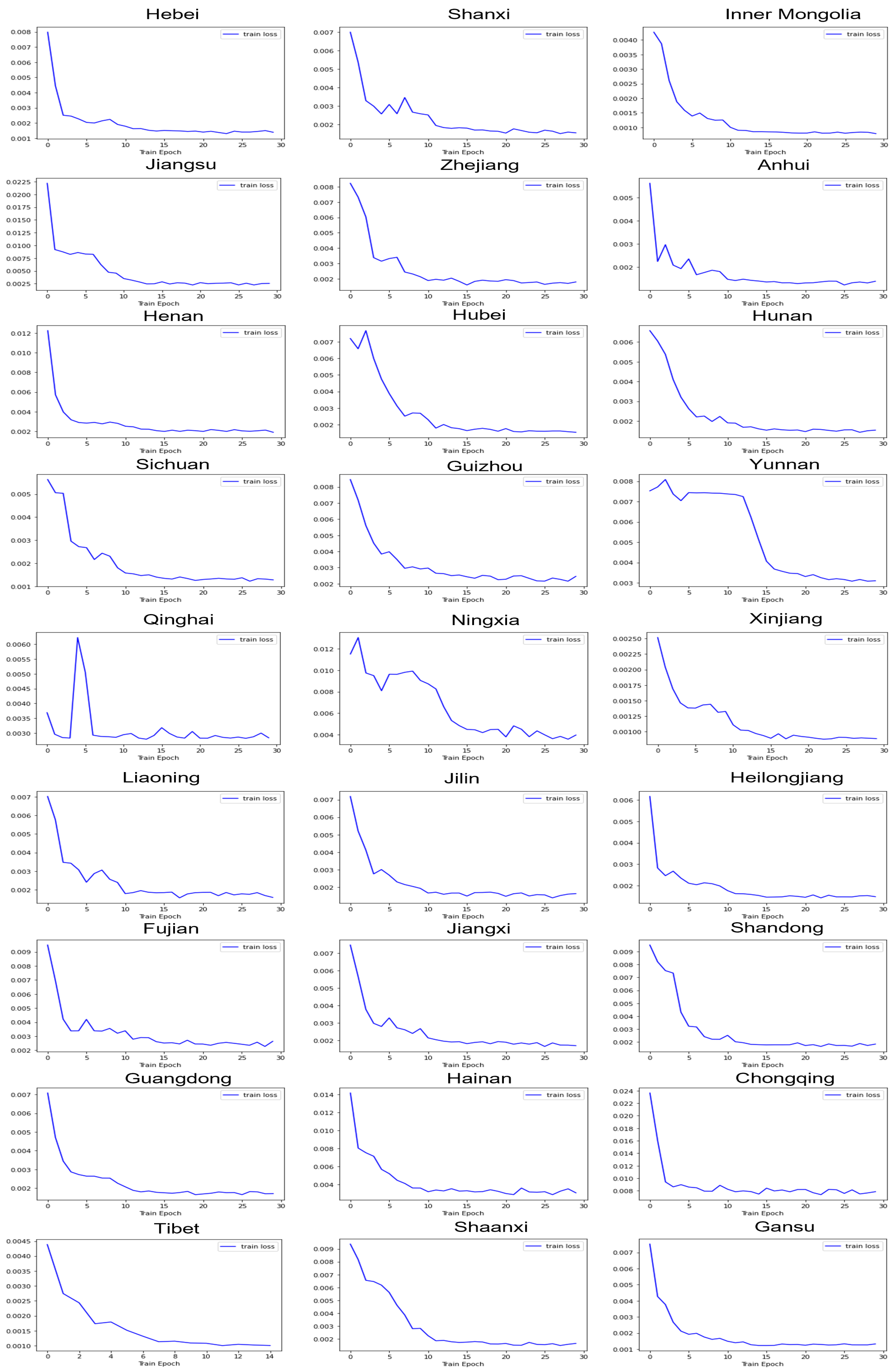
The convergence of the model is shown in Figure 10. From the figure, we can see that the curves eventually all tend to be smooth, but Yunnan, Qinghai, Ningxia and other regions show abnormal fluctuations in the loss curves during the model training. Through observation and analysis, we found that the fluctuation of the learning rate may result in these fluctuations. The learning rate is a parameter that controls the update rate of the model parameters, and when the learning rate changes, the update rate of the model parameters will also change, and this change may lead to a turning point in the training of the model. Because our learning rate automatically declines through adjustment after a period of training epochs, some fluctuations occur during the training process, and eventually the loss values all tend to converge. Dynamically adjusting the learning rate can adjust the learning rate in real time according to the performance of the model, enabling the model to obtain better gradients during training, thus improving the accuracy of the model, accelerating the convergence of the model, and enabling the model to obtain better generalization on both the training and test data.

4.2. Projected Results for Different Provinces

China is a vast country with great differences in topography and climate among provinces, and water resources are unevenly distributed [36]. In order to take full advantage of the favourable conditions in each region to increase the total amount of grain yield. In different regions and seasons, farmers choose to grow different grain crops. These include summer grain, early rice and autumn grain, cereals, legumes and potatoes.

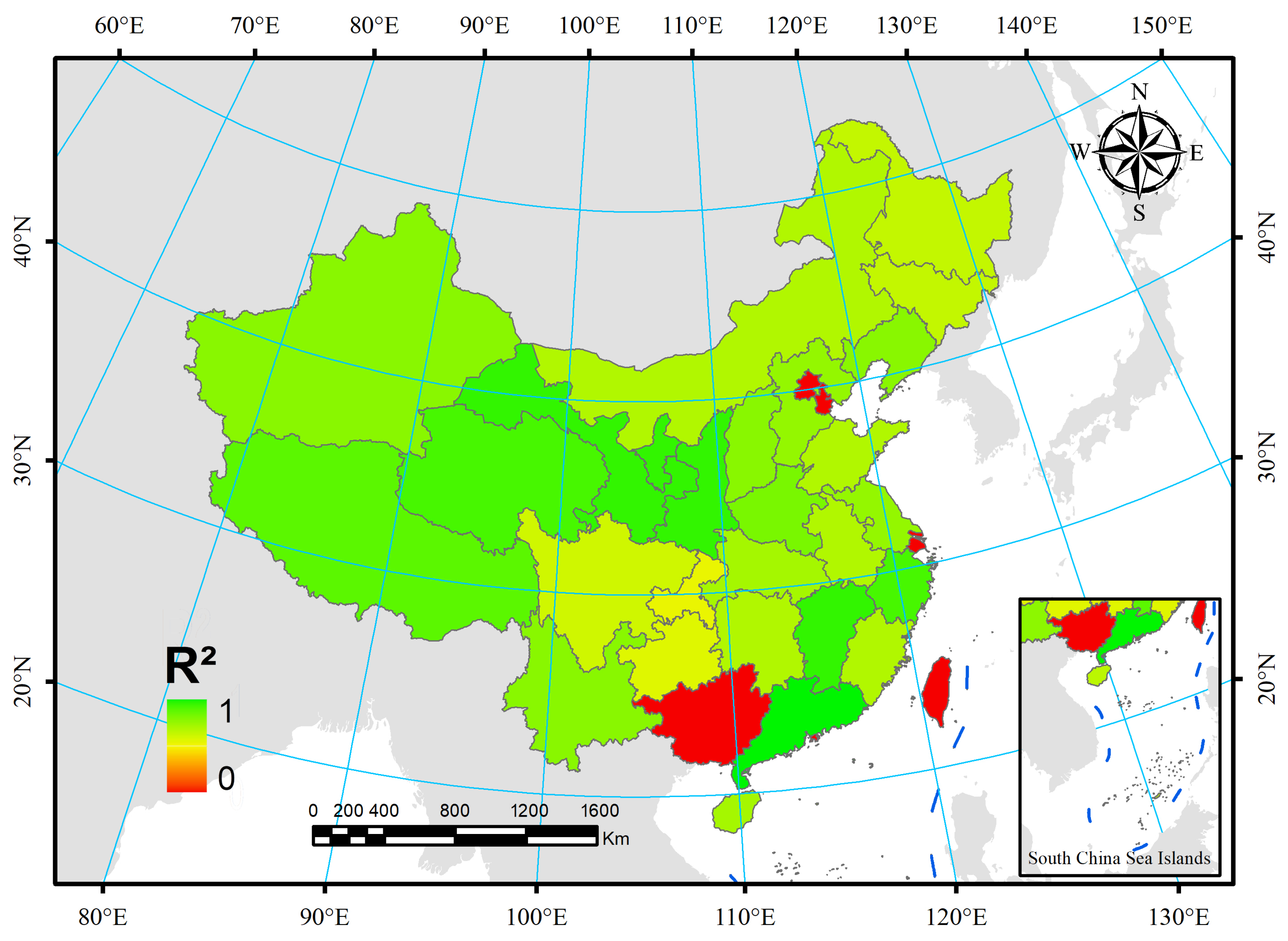
To verify the robustness of our proposed neural network model for predicting multiple grain crops in different regions, we calculated the yield prediction accuracy of different provinces separately (Figure 11). The results in the figure show that in some provinces the yield estimation accuracy is low, but in most cases the accuracy is satisfactory. For example, Guangdong has the highest accuracy with ${\mathrm{R}}^2$ of 0.989 and RMSE of 18,040 tons, and the lowest is in Chongqing with ${\mathrm{R}}^2$ of 0.815 and RMSE of 132,370 tons. This proves that our proposed neural network model has good robustness.

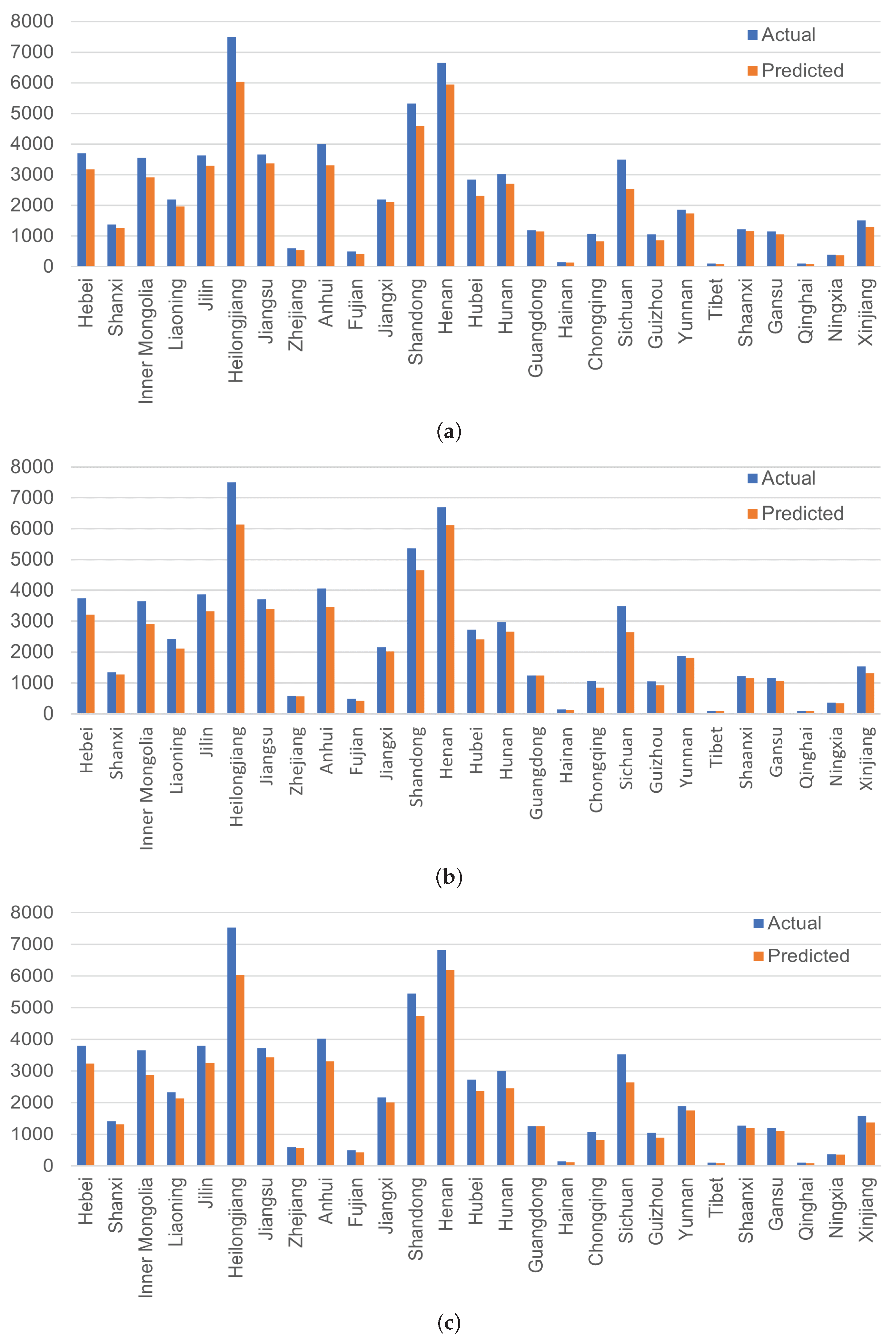
The predicted and actual yields for 2018–2020 are shown in Figure 12 and

Table 3. 2018–2020 model prediction accuracy by province.

Country	2018		2019		2020
	${\mathbf{R}}^2$	RMSE	${\mathbf{R}}^2$	RMSE	${\mathbf{R}}^2$	RMSE
Hebei	0.942	11.708	0.944	11.644	0.940	12.272
Shanxi	0.941	4.469	0.953	3.915	0.944	4.476
Inner Mongolia	0.938	4.606	0.927	5.117	0.917	5.462
Liaoning	0.946	7.933	0.922	10.605	0.955	7.772
Jilin	0.915	14.782	0.901	17.027	0.892	17.413
Heilongjiang	0.910	15.215	0.920	14.381	0.908	15.427
Jiangsu	0.943	18.020	0.941	18.612	0.944	18.238
Zhejiang	0.962	2.933	0.983	1.954	0.977	2.285
Anhui	0.891	24.045	0.923	20.500	0.903	22.727
Fujian	0.892	3.087	0.937	2.331	0.916	2.745
Jiangxi	0.985	4.725	0.972	6.322	0.970	6.473
Shandong	0.919	19.449	0.924	19.001	0.924	19.313
Henan	0.947	20.401	0.957	18.650	0.955	19.334
Hubei	0.894	16.741	0.941	11.987	0.941	12.056
Hunan	0.9486	8.954	0.935	10.097	0.875	13.957
Guangdong	0.9809	2.2982	0.9893	1.7854	0.9879	1.9398
Hainan	0.919	2.567	0.956	1.876	0.901	2.814
Chongqing	0.792	13.909	0.824	12.756	0.812	13.617
Sichuan	0.847	16.122	0.887	13.904	0.873	14.818
Guizhou	0.697	7.686	0.903	4.351	0.830	5.606
Yunnan	0.961	2.767	0.975	2.216	0.961	2.846
Tibet	0.967	0.270	0.971	0.255	0.975	0.231
Shaanxi	0.973	2.573	0.974	2.535	0.973	2.649
Gansu	0.976	1.918	0.977	1.896	0.976	2.010
Qinghai	0.970	0.562	0.973	0.544	0.974	0.549
Ningxia	0.974	2.461	0.973	2.377	0.970	2.573
Xinjiang	0.958	2.018	0.959	2.011	0.959	2.094

, from which it can be visualized that in some provinces with large grain production, such as Heilongjiang, Henan and Shandong, the model correctly predicts the yield trend, but there is a gap between the predicted and actual yields. There are many potential factors that could influence the accuracy of a grain yield prediction model in different provinces, including variations in local climate, soil conditions, and agricultural practices. The model’s ability to capture these differences and accurately predict grain yield may depend on the quality and quantity of data available for training and testing, as well as the specific techniques and algorithms used in the model. It is also possible that the model’s performance may be influenced by other factors, such as the availability and accuracy of real ground data for validation, or the specific crops and varieties grown in different provinces.

During the 2018–2020 period, our prediction model also shows some fluctuations in predicted values, in addition to provinces with relatively high or low actual grain yields. This may be due to the structural reform of the supply-side of Chinese agriculture, which aims to improve the quality and efficiency of grain production by adjusting the cropping structure. Different provinces can adjust the acreage of different crops according to their local geographical and climatic factors. However, the land classification masks used in our model are fixed and may not be able to fully take into account these variations, leading to errors in the processed remote sensing images and eventually the fluctuations in the prediction results.

4.3. Ablation Experiment

To verify the validity of each module in this model, ablation experiments were conducted. Tests were also conducted separately for each year to accurately test the predictive ability of the present model. As can be seen from

Table 4. Results of ablation experiments.

Item	2018		2019		2020		Average
	${\mathbf{R}}^2$	RMSE	${\mathbf{R}}^2$	RMSE	${\mathbf{R}}^2$	RMSE	${\mathbf{R}}^2$	RMSE
CNN	0.834	12.589	0.848	12.240	0.840	12.157	0.851	11.905
CNN + CBAM	0.883	10.155	0.900	9.441	0.889	9.738	0.899	9.362
CNN + LSTM	0.896	9.836	0.918	9.288	0.897	10.393	0.910	9.548
CNN + CBAM + LSTM (Ours)	0.926	8.601	0.942	8.098	0.932	8.581	0.940	8.002

, our average ${\mathrm{R}}^2$ is 0.940 and the average RMSE is 80,020 tons on the test data from 2018 to 2020. Compared to the CNN, our model predicts an improved ${\mathrm{R}}^2$ of 0.089 and a reduced RMSE of 39,020 tons, a significant improvement in these metrics. Meanwhile, the inclusion of LSTM is better compared to the inclusion of CBAM, but the difference between them is not significant.

5. Discussion

In recent years, the concept of sustainable development has been widely accepted and implemented in many fields. In particular, many countries are actively addressing food security, climate change, environmental protection and resource use. However, the challenges to the development of sustainable agriculture are also significant. Global food security has deteriorated in the past few years. Climate change, natural disasters, market volatility, and policy instability have all contributed to high food prices and increased food insecurity. In addition, global population growth and urbanization have exacerbated food security issues. Despite the enormous challenges, many countries and organizations are taking steps to address these issues. Only global cooperation and joint efforts can ensure globally sustainable development and food security.

Our study stands out from previous ones in its approach to learning features directly from the original bands using the attention module. Unlike previous studies that only averaged or sampled the vegetation indices, our model preserves essential information on spatial variation during plant growth. Additionally, our study has a larger scale and higher accuracy, making it a valuable contribution to the field.

Because different food crops have different growth cycles, some regions often grow crops that span two years. For example, in the North China Plain, winter wheat is planted from October to December each year and only matures for harvest in the middle of the following year. However, our data samples are constructed based on each calendar year rather than on the crop growth cycle. Still, the model shows good accuracy for yield prediction, which we attribute to the fact that the actual yield data in the Statistical Yearbook are also based on calendar years. In subsequent research work, we could change the time series of the data sample to two or even three years instead of the currently used one year. This includes data for the complete cycle of each crop from sowing to harvest and may give us more accurate results. In addition, some of the remote sensing data variables selected in our study (Table 1) are selected empirically and based on the summaries of previous studies by some scholars, and their relevance to grain yield is not explored in depth, but this highlights the effectiveness of neural networks in end-to-end problem studies.

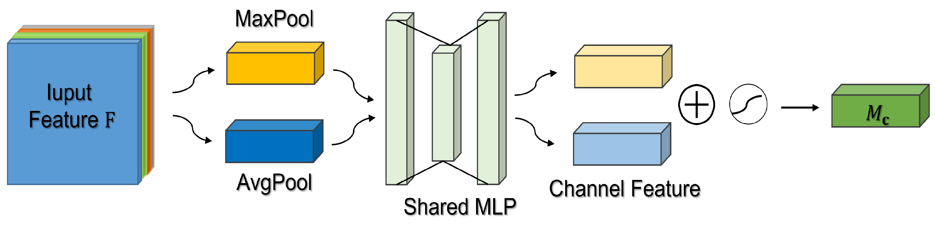
The attention mechanism in a neural network model allows it to selectively focus on certain input features or patterns, which can be particularly useful in situations where the input data are complex or large. In the context of a grain yield estimation model, the attention mechanism can be used to improve the model’s performance by helping it to better capture and utilize relevant patterns or features in the data, such as vegetation index and temperature, that are known to influence grain yield. For example, the vegetation index, which is a measure of the density and health of vegetation, is an important factor in grain yield prediction. By using the attention mechanism to focus on this feature, the model can more accurately capture the relationship between the vegetation index and grain yield, leading to more accurate predictions. Similarly, temperature is also known to affect grain yield, and the attention mechanism can be used to focus on temperature data to improve the model’s ability to predict grain yield based on temperature. Overall, the attention mechanism can improve the performance of a grain yield estimation model by allowing it to more accurately capture and utilize relevant patterns or features in the data.

The fluctuations in the prediction values observed may be due to the use of an inappropriate land classification mask for the corresponding year. Initially, we planned to use the land classification mask from the moderate resolution imaging spectroradiometer (MODIS) MCD12Q1 product, but this product has relatively large errors in the distribution of grain crops in China. In comparison, the land-use mask from the Institute of Geographic Sciences and Natural Resources Research of the Chinese Academy of Sciences has been manually verified and is more representative of the actual conditions, but may not be available annually due to the large workload involved in its production.

Upon reviewing Cao et al.’s research [37] predicting winter wheat yield, we have taken note of their comprehensive consideration of soil, climate, elevation, and human factors. This serves as a valuable reference for our own future research endeavours. However, we must now address the challenge of expanding the “point” data on soil and human influence to a larger, more comprehensive “surface” level. This will require careful consideration and planning in order to accurately incorporate these factors into our research methodology. We remain committed to advancing our understanding of crop yield prediction and will continue to draw upon the insights of previous research in pursuit of this goal. In addition, Valjarevic et al. [38] conducted a study on forest tree density using pixel and sub-pixel analysis. It is our opinion that their methodology can be utilized for yield research purposes to enhance the precision of data. This approach may prove to be an effective means of improving accuracy in the field of agriculture.

In our study, the attention mechanism shows strong performance in learning crop yield features, and we could potentially apply the attention mechanism to the learning of farmland distribution features and further reduction in the errors. By focusing on relevant features, the attention mechanism can help the model to more accurately capture and utilize the patterns or characteristics that influence the prediction task. In this case, applying the attention mechanism to the learning of farmland distribution features could potentially help the model to better capture the changes in planting structures and land use that may have contributed to the observed fluctuations in the prediction values.

6. Conclusions

Our study highlights the importance of accurate grain yield prediction for ensuring global food security and demonstrates a novel approach that can contribute to this goal.

There is a connection between the methods of remote sensing and attentional mechanisms in grain yield analysis. Attentional mechanisms are cognitive processes that allow to selectively focus on relevant information while ignoring irrelevant information. In the context of remote sensing, attentional mechanisms can be used to identify and extract important features from the images captured by sensors. For example, spectral analysis involves the identification of specific bands of light that are absorbed or reflected by crops, which can be used to estimate crop health and yield potential. By selectively attending to these bands, remote sensing techniques can provide valuable information for grain yield analysis. Similarly, land surface temperature involves the detection of heat signatures emitted by crops, which can be used to estimate biomass and yield potential. Attentional mechanisms can be used to identify and extract these heat signatures from the images captured by sensors, providing valuable information for farmers to make informed decisions about crop management and harvest planning.

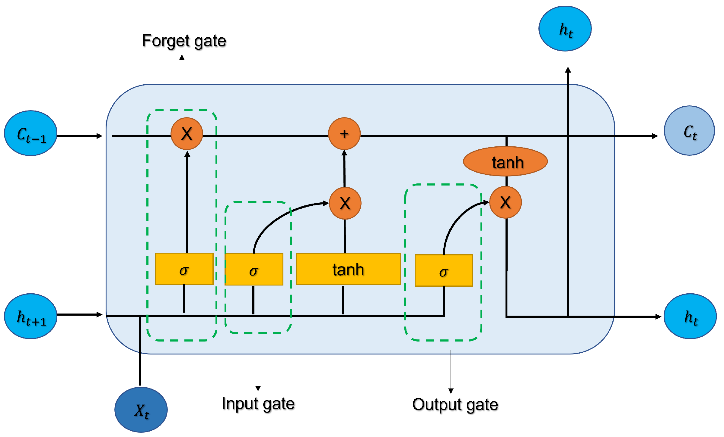
In order to make grain yield prediction less costly and improve the accuracy of grain yield prediction at the same time, a hybrid neural network grain yield prediction model is proposed in this paper. The underlying data used in the model are from MODIS satellite products, and we combine information from different bands into composite remote sensing image data to provide as many training features as possible for the model. Then, based on the convolutional network as the base structure, we use the attention of channel and spatial mixing to enhance the extraction of the vegetation index and temperature-associated features. Finally, we use LSTM to process the data of each month to obtain as much information as possible in the temporal dimension. Through experiments, we find that the proposed model in this paper has an ${\mathrm{R}}^2$ of 0.940 and an RMSE of 80,020 tons for grain yield prediction in China, a large improvement in yield prediction compared with the traditional convolutional network. We also calculate the accuracy of grain yield prediction for different provinces one by one, where Guangdong province has the most accurate grain yield prediction with ${\mathrm{R}}^2$ of 0.989 and RMSE of 18,040 tons, while Chongqing city has the worst prediction accuracy with ${\mathrm{R}}^2$ of 0.815 and RMSE of 132,370 tons. Compared to previous studies, the attention mechanism-combined LSTM model is more accurate in predicting Chinese grain yield in an end-to-end manner on a large scale. Furthermore, providing an effective technical method for agricultural testing and grain yield estimation.