Abstract
In order to promote the cost reduction and efficiency improvement of the logistics distribution process and to guarantee the safety of goods transportation, this paper studies the portfolio optimization of goods loading and the problem of simultaneous pickup and delivery vehicle routing. A balanced loading constraint was introduced to restrict loading through two aspects of axle weight bearing and lateral center-of-gravity offset. With the shortest total route length as the objective, this paper constructs a simultaneous pickup and delivery vehicle routing model with three-dimensional (3D) balanced loading constraints (3BL-VRPSPD). Additionally, a hybrid tabu search (TS) algorithm embedded loading test was proposed to solve this problem. Firstly, a heuristic insertion method was applied to determine the initial routing scheme, and the node swapping and relocation operators were designed to construct the tabu neighborhood scheme for routing optimization. On this basis, the 3D balanced loading was incorporated into the routing iteration process. A balanced loading algorithm, combining multiple-indicator ordering and maximum space division strategies (MOMD), was formulated to develop a 3D-balanced loading plan for goods with a pickup and delivery vehicle routing scheme. Finally, standard instances verified the effectiveness of the method. The results show that the proposed method can effectively optimize 3BL-VRPSPD and outperform other algorithms.
1. Introduction
As an important part of the modern logistics system, transportation and distribution services assume a significant role in supporting economic and social development. At present, transportation costs still occupy the largest part of the total cost structure of social logistics. Sustainable social and economic development is constrained by high logistics costs. Thus, it is clear that cost reduction and efficiency improvement are urgent issues to be solved in the logistics and transportation industry [1,2]. The vehicle routing problem (VRP) and goods loading layout problem are important aspects of the logistics distribution process, and the portfolio optimization of these two problems is of great significance for cost reduction and efficiency improvement.
As an extension of the VRP, the simultaneous pickup and delivery vehicle routing problem (VRPSPD) is an abstract representation of a complex distribution model. The VRPSPD means that both the pickup and delivery tasks need to be completed at each customer node. So, it is widely used in several fields, particularly in situations where customer pickup and delivery needs are separated [3,4]. For example, in the courier industry, parcels are delivered to customers while also providing pickup services. In addition, in the food, electronics, automotive and other industrial manufacturing industries, the raw materials provided by the supply chain need to be picked up and returned to the warehouse, while the manufactured products need to be delivered to the customers. In addition, as environmental issues are of wide concern, the closed-loop system of “resource-product-recyclable resource” is widely used. The delivery of goods not only needs to deliver products to customers, however, it also needs to recycle various kinds of packaging or used parts to realize the recycling of resources. In an actual distribution scenario, the goods transported by the vehicles have three-dimensional (3D) dimensions, as well as weight attributes. In particular, goods with large volumes can easily result in irrational layout schemes, leading to the predicament of satisfying the volume loading limit but still being unable to load, resulting in wasted space. Therefore, when studying the VRPSPD, it is necessary to consider not only the traditional routing constraints but also the 3D loading constraints. Moreover, in the field of goods transportation, where high demands are placed on the center of gravity balance, such as in the transportation of household appliances, furniture, and construction materials, ensuring the safety of goods transportation is critical in improving the durability and service life of the vehicle.
This paper proposes the simultaneous pickup and delivery vehicle routing problem with 3D balanced loading (3BL-VRPSPD). In particular, a dynamic balance loading constraint is introduced. It includes two parts: the axle weight support constraint and the lateral center-of-gravity offset constraint. The axle weight support constraint is to limit the distributed stress of goods loading so that the load in the vehicle compartment meets the requirements of each axle’s load-bearing capacity. The lateral center-of-gravity offset constraint is to limit the total center-of-gravity range of the goods in the carriage. This is carried out to reduce or avoid an excessive center-of-gravity shift and stress concentration due to the process of cargo transportation so as to improve the safety and stability of the goods distribution process.
Currently, there are more studies focused on vehicle routing optimization, while vehicle scheduling optimization that integrates two critical factors of 3D loading and simultaneous pickup and delivery is less commonly studied. However, in reality, the distribution problem faced by logistics enterprises often involves a combination of the two aforementioned problems. Therefore, this paper aims to integrate the consideration of 3D loading and simultaneous pickup and delivery while also introducing balanced loading constraints to make the problem more applicable and realistic. The overall framework of this study is shown in Figure 1.
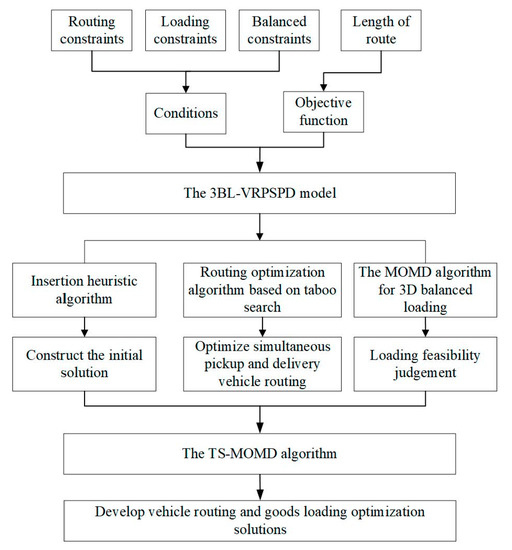
Figure 1.
Flow chart of the research.
The structure of this paper has been organized in the following manner: Section 2 presents a comprehensive Literature Review, which offers a summary of current research on the VRPSPD. The review offers a horizontal comparison and proposes the research direction for this paper. Section 3 offers a Problem description and Model Construction, which outlines the VRPSPD and goods loading optimization concepts. In this section, the balanced loading constraint is also introduced, and a comprehensive model is established. Section 4, Model Solving Algorithm Design, analyzes the complexity of the problem and proposes a hybrid heuristic algorithm with the tabu search (TS) framework embedded with loading tests. Section 5, Case Study, validates the proposed method by applying standard case scenarios and verifies the algorithm effect by comparing different algorithms. Finally, Section 6, Conclusion, summarizes the main findings of the paper and proposes key research directions for future studies.
2. Literature Review
With the development of logistics, the VRP has received more and more attention and has gradually developed into a rich and active research area. It was first proposed by Dantzig and Ramser in 1959 [5]. With the in-depth study of practical problems, a large number of variant studies have been generated on the basis of the traditional VRP, such as the capacitated vehicle routing problem (CVRP) [6], vehicle routing problem with time window (VRPTW) [7], vehicle routing problem with simultaneous pickup and delivery (VRPSPD) [8]. At the same, a large amount of research attempts have been devoted to designing efficient optimization methods in order to improve the solving efficiency for this problem, such as nested and joint algorithms [9], genetic algorithms [10,11], large neighborhood search algorithms (LNS) [12], hybrid metaheuristic algorithm [13], ant colony optimization algorithm [14], grey wolf optimization algorithm [15] and so on. Abbaspour and Aghsami [16] conducted a comprehensive comparative analysis of the performance of 13 different meta-heuristic algorithms, including the dragonfly algorithm and the grasshopper optimization algorithm. These algorithms gradually improve the solvency and efficiency of the VRP.
As an important extension of VRP, VRPSPD is an abstract representation of a complex distribution model that is also receiving increasing attention from scholars. This problem was first proposed by Min [17] in 1989. On this basis, scholars have studied the extension problems for VRPSPD, which include the introduction of time window constraints, VRPSPD with heterogeneous fleet, green VRPSPD, stochastic VRPSPD and so on.
Angelelli and Mansini [18] introduced the VRPSPD with time windows and proposed a branch-and-cut-and-price algorithm. Liu and Tang [19] proposed a novel memetic Algorithm with an efficient local search and extended neighborhood to solve the VRPSPD with time windows. Jin and Li [20] investigated a special VRP with realistic constraints, including product classification, pickup–delivery, and time windows, in addition to proposing a hybrid algorithm combining tabu search and artificial immune algorithms.
Avci and Topaloglu [21] extended VRPSPD by assuming that the fleet is heterogeneous and developed a hybrid local search algorithm that combines a non-monotonic threshold adjustment strategy with TS. Their threshold function has an adaptive property capable of self-adjustment. Nepomuceno and Saboia [22] proposed a fast randomized algorithm using the nearest neighbor strategy to tackle an extension of the VRPSPD in which the fleet of vehicles is heterogeneous.
In recent years, numerous researchers have focused on the study of green VRP and have expanded their focus to include the green VRPSPD.
Li [23] studied green VRPSPD in the context of steel distribution and designed a mixed-integer linear programming model. The improved intelligent water drop algorithm was applied, which was compared with the genetic algorithm to verify its practicality. Qu and Zhang [24] investigated VRPSPD in the context of green cold chain logistics. A multi-objective optimization model considering carbon emission, route cost, and time window was constructed. Furthermore, the multi-objective optimization algorithm with multiple neighborhood operator searches was designed to solve it.
As for stochastic VRPSPD, Hou and Hong [25] designed a discrete difference evolutionary algorithm to solve the routing optimization model. Subsequently, Zhang [26] constructed a chance-constrained programming model to treat the problem statically, with the scattering search algorithm designed to construct the solution.
On the other hand, VRPSPD has been investigated by studying different solution algorithms, and the research results can be classified into three categories: exact solution algorithms, heuristic algorithms and intelligent optimization algorithms.
Subramanian worked on solving this problem using exact algorithms. In 2011 [27], a lazy branch-and-shear algorithm for the VRPSPD was proposed. In 2013 [28], a branch pricing algorithm was proposed for the VRPSPD, validated on a public dataset. Although exact algorithms for VRPSPD have been able to solve instances with up to 200 customer points, the prohibitive runtime has also led the research direction toward intelligent heuristic algorithms. Dethloff [29] was among the first researchers to use heuristic algorithms to study the VRPSPD. They pointed out the importance of VRPSPD in reverse logistics and proposed an algorithm based on the sparing insertion method, which also provided a common dataset for the VRPSPD. Kalayci [30] designed a hybrid heuristic algorithm to solve VRPSPD. The storage structure of the ant colony system was used in conjunction with the variable neighborhood search algorithm (VNS) to provide a perturbation mechanism for the algorithm using pheromones. Zhang and Chen [31] proposed a novel dynamic multi-stage failure-specific cooperative (DMS-FSC) recourse strategy for solving the route failure which occurs in the VRPSPD. Additionally, they designed an extended genetic algorithm with a new multi-stage paired vectors representation scheme that is offered to deal more effectively with the proposed DMS-FSC strategy. Oztas and Tus [32] proposed a hybrid algorithm combining the iterated local search, variable neighborhood descent and threshold acceptance metaheuristics to solve the VRPSPD. Yu and Aloina [33] cast the VRPSPD into a mixed-integer linear programming model and proposed a simulated annealing heuristic with a mathematical programming-based construction heuristic to solve the VRPSPD.
In summary, considerable progress has been made in the extension problem and algorithm optimization of VRPSPD. Various heuristic algorithms have been developed to solve the problem and have achieved promising results, which provide a solid foundation for further research. However, research on the problem of VRPSPD with 3D loading is relatively scarce, and little attention has been given to balanced loading constraints, which involve the safety of loading and unloading during the goods transportation process. Since 3BL-VRPSPD can closely reflect actual distribution scenarios and improve the safety of goods transportation, optimizing the combined problem is critical to practical logistics and distribution and has important applications in the field of logistics and distribution. Therefore, it is necessary to explore optimization theories for this problem by integrating practical constraints.
3. Materials and Methods
3.1. Problem Description
The 3BL-VRPSPD is shown in Figure 2 and can be described as follows: For a distribution center, there are a certain number of the same types of vehicles to serve customers and meet the customer’s pickup and delivery demand simultaneously. The quantity of goods that each customer needs for delivery and pickup is determined. The distribution centers assign vehicles to visit customers according to the order requirements. These distribution centers need to comprehensively consider and make rational decisions on the distribution vehicles, the distribution sequence, schemes and goods-loading solutions under the constraints of satisfying the demands of the customers, the maximum loading capacity of the vehicles, and 3D balanced loading limitations, to achieve the goal of the shortest total vehicle routing.
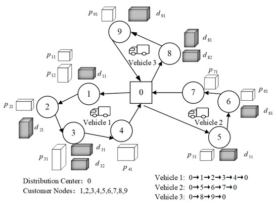
Figure 2.
Schematic diagram of the 3BL-VRPSPD.
Therein, the assumptions of the 3BL-VRPSPD are listed as follows: (i) There is only one distribution center, which is the starting and ending point of the vehicles; (ii) the vehicles at the distribution center are all tail-loading trucks of the same specifications; (iii) each customer is visited by the vehicle only once, and the empty vehicle can satisfy the demands of a single customer; (iv) the goods have homogeneous, rectangular shape characteristics, the center of gravity of the goods is located in the geometric center and the goods cannot be moved during transit.
3.2. Notations
For easy reference, this section gives the description of notations that will be used in this paper, which are listed in Table 1.

Table 1.
Description of notations.
3.3. Formulation of the 3BL-VRPSPD
Based on the comprehensive considerations above, with the shortest total vehicle travel path as the optimization objective, the optimization model of 3BL-VRPSPD is constructed as follows:
which is subject to:
Equation (1) indicates the objective function, which is the shortest route length. Equations (2) and (3) indicate that each node can be visited only once. Equation (4) indicates that the customers on each route can only be visited by the same vehicle. Equations (5)–(7) indicate that each vehicle starts and ends at the distribution center. Equation (8) indicates the maximum vehicle mileage constraint. Equation (9) indicates the avoidance sub-circuit. Equation (10) indicates the load constraint of the vehicle. Equations (11) and (12) indicate the flow conservation constraint for pickups and deliveries. Equation (13) indicates the non-negative volume of pickups and deliveries for each customer. Equations (14) and (15), respectively, indicate that the total weight and volume of the goods do not exceed the rated weight and effective volume. Equation (16) indicates that the position of the cargo cannot overlap. Equation (17) indicates that the goods cannot be overhanging. Equation (18) indicates that the goods cannot exceed the effective loading space of the vehicles. Equations (19) and (20) are support-surface constraints. Equation (21) is the fragility constraint, as only fragile goods can be placed above the fragile goods, and non-fragile goods above the fragile goods are not required. Equations (22) and (23) indicate the vehicle longitudinal-axle-weight constraint. Equation (24) indicates the goods’ lateral center-of-gravity offset constraint.
4. Model-Solving Algorithm Design
4.1. Framework of the Solution Mechanism
The solution of 3BL-VRPSPD involves two aspects, namely, the route planning of the pickup and delivery vehicles and the 3D balanced loading of goods at nodes. Therefore, this paper proposes a hybrid heuristic algorithm with TS as the framework embedded in the goods loading link. It is proposed to incorporate goods loading into the inspection link of route planning and integrate the feasibility judgment of 3D balanced loading into the routing optimization process. In this paper, we use TS to optimize the routing and design a 3D balanced loading algorithm based on multiple-indicator ordering and maximum space division (MOMD) to complete the goods loading of nodes. The proposed algorithm of simultaneous pickup and delivery vehicle routing optimization is based on TS with 3D balanced loading (TS-MOMD). The basic flow of the algorithm is shown in Figure 3.
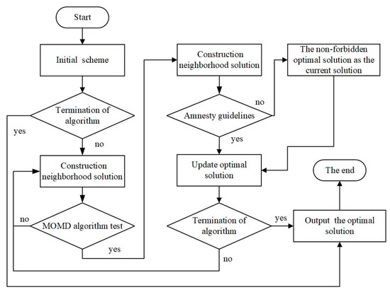
Figure 3.
Algorithm framework diagram.
4.2. The Design of TS-MOMD Algorithm
4.2.1. Initial Solution Construction
The problem characteristics are analyzed, and feasible initial solutions are constructed using an insertion heuristic algorithm. In this way, high-quality initial solutions are obtained to lay the foundation for subsequent TS.
Firstly, start a vehicle, select the customers that are feasible to load, and if there are multiple customers that can be loaded, select the customer with the shortest distribution routing to form the distribution route , i.e., select the customer with the smallest routing length to insert into the routing.
Then, among the currently unloaded customers, select the customer with loading feasibility. If there are multiple loadable customers, the customer with the shortest routing is selected. Assume that the existing distribution route is and the distribution routing is formed after loading customer . Select the customer node with the largest path-saving value and insert the routing. If there is no customer that meets the feasibility of loading, then move to the previous step. If all customers are loaded, then output the initial routing scheme .
4.2.2. Neighborhood Structure Construction
Independent parallel node swapping and relocation operators are designed to construct neighborhood schemes based on intra-routing and between different routings. The operator is shown in Figure 4.
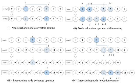
Figure 4.
Schematic diagram of the neighborhood operator.
- 1.
- Node exchange operator within routing
Select a transport routing in the current routing scheme, and randomly select two customer nodes in that routing to exchange and form a new route. Take the example shown in Figure 4, the randomly select route 1, then randomly select customer nodes and in that routing, and exchange nodes and to form a new routing route 1′.
- 2.
- Node relocation operator within routing
Select a transport routing in the current scheme, select consecutive customer nodes of that routing, and relocate these nodes to form a new route. If , randomly select a node and insert it into other positions of this routing. When , randomly select route 1 in the current scheme, relocate nodes and of route 1 to between nodes and to form a new route. As shown in Figure 4, if more than one position can satisfy the constraint, the position with the smallest route length is selected to insert the node.
- 3.
- Inter-routing node exchange operator
Select two routes in the current scheme, select a node in each route respectively, and form two new routes after the exchange. As shown in Figure 4, after selecting route 1 and route 2, node is randomly selected from route 1, node is randomly selected from route 2, and node and node are exchanged to form two new routes. If more than one position can satisfy the constraint, the position with the smallest route length is selected to insert the node.
- 4.
- Inter-routing node relocation operator
Select two routes in the current scheme, select a node at random from one and insert it into the other to form two new routes. As shown in Figure 4, node is randomly selected from route 1 to transfer between node and of route 2 to form two new routes. If more than one position can satisfy the constraint, the position with the smallest route length is chosen to insert the node.
4.2.3. The MOMD Algorithm for 3D Balanced Loading
The key of the MOMD algorithm is the matching of the effective loading space and 3D goods. In this paper, this is achieved by designing a multiple-indicator ordering strategy and a maximum-space-division positioning strategy. This algorithm is used to perform goods loading at each node and is used to test the optimized routing scheme.
- 1.
- Loading and positioning rules
The goods loading and positioning consists of three parts: the division of load space, update of load space and selection of available space. In this paper, the maximum space division (Figure 5) method represents the remaining space; set F is defined to represent the loadable space. The original loadable space is the whole rectangular carriage, and after the first goods are placed in the carriage, the remaining space is divided into three maximum covering rectangles according to the maximum space partitioning idea.

Figure 5.
Schematic diagram of the maximum space division method.
For the space update, when the goods of the delivery space are delivered to the node, and if two planes of this space coincide with the bottom and front of the carriage, respectively, the pickup space is transformed for loading the goods, and then the set F of available spaces is updated.
The rule of selecting the loadable space is in the order of the available space coordinates . When loading the goods, the loading space for trying the next piece of the goods is selected according to the principle of front to back, bottom to top and left to right.
- 2.
- Loading and ordering rules
Based on the multiple-index ordering strategy, four loading sequences are obtained by sorting the goods according to weight, volume, bottom area from large to small and fragility from small to large. Sequence selection was performed in the order of weight > volume > bottom area > friability.
- 3.
- Design of MOMD algorithm
In this paper, based on the multi-index ordering strategy and maximum-space partitioning strategy, the 3D balanced cargo-loading algorithm (MOMD) is designed as follows:
Input: goods information
Output: the loading scheme and the remaining space set
Step 1: Define the goods set of customers as , the goods loading scheme set of is , initialize , , ;
Step 2: Based on the multi-index ordering strategy, the goods are sorted by weight, volume, bottom area, and fragility. In order to obtain four sets of loading sequences ;
Step 3: Load the goods according to the first sequence in the set of loading sequences ; use to sort the goods to obtain ; if all sequences have been tried, i.e., , turn to Step 7. Otherwise, remove this sequence from the set and update the set , and turn to Step 4;
Step 4: Load goods of according to the maximum space partitioning strategy. If , turn to Step 6, otherwise, turn to Step 5;
Step 5: If is successfully placed in the load space and the load constraint is satisfied, remove it from the set , update and turn to Step 4; otherwise, the load is deemed to have failed and the next load sequence is attempted, in which case, turn to Step 3;
Step 6: Perform a balanced loading test on the loaded goods. If passed, determine that the goods of customer is successfully loaded, and update the set of goods loading solutions and , and turn to Step 7, otherwise, to Step 3;
Step 7: If , it means that the goods of customer are not loaded successfully, otherwise, it means successful loading, and output the loading scheme and the remaining space set .
4.2.4. Design of TS-MOMD Algorithm
The TS is an iterative search algorithm that seeks progressively superior neighborhoods and utilizes memory to guide the search process. In this study, four types of domain construction methods are designated as tabu objects; the objective function serves as the evaluation criterion for the solution. When a neighborhood solution is searched, the objective function formula is used to evaluate the solution by computing the length of its total route. Based on problem characteristics and experimental calculation results, the maximum number of iterations for TS is set as the stopping criterion. The proposed TS-MOMD algorithm is as follows:
Input: set of customers , set of goods , rated by weight , carriage length , width and height ;
Output: optimal solution , objective function value ;
Step 1: The initial routing scheme is generated, and its corresponding loading scheme is , both of which form a temporary solution . Initialize the taboo table , taboo length , maximum number of iterations , number of iterations , current optimal solution .
Step 2: Generate the set of routing neighborhood schemes , using the intra-route node exchange operator, intra-route node relocation operator, inter-route node exchange operator and inter-route node relocation operator.
Step 3: The MOMD algorithm is called to perform the loading test on . If it can complete the loading of goods at all nodes and satisfy the 3D balanced loading constraint, the loading scheme is obtained, and the routing scheme and the loading scheme together constitute the neighborhood solution, go to Step 4; if the test is not passed, the node exchange or repositioning of the original route is removed, go to Step 2.
Step 4: The solution evaluation criterion is applied to rank the neighborhood solutions. If the optimal neighborhood solution meets the amnesty criterion, i.e., the route length of optimal neighborhood solution is less than the , the optimal neighborhood solution is assigned to ; otherwise, the remains unchanged.
Step 5: If the route length of the current temporary solution is better than the current optimal solution, then . Add the taboo objects of S to the , update the and .
Step 6: Determine whether the iteration count termination rule is satisfied; if , the algorithm terminates and outputs the and , otherwise, it continues to execute Step 2~Step 6.
5. Computational Experiments
The experiments and experimental results based on a large number of widely used VRPSPD instances are given and compared with existing methods. The algorithm is coded with JAVA, using the IntelliJ IDEA platform, and the experimental machine is configured with Windows 10 Professional 64-bit OS, which runs on an Intel(R) Core (TM) i54200M @ 2.50 GHz, 8.0 GB RAM PC.
5.1. Testing Instances and Parameters
In this paper, we adopt the classical VRPSPD test dataset proposed by Salhi S [34]. We selected 14 data sets from CMT1X-CMT14X. The size and serial numbers of the instances and the number of customer nodes per set of instances are shown in Table 2. Since the initial data set does not have data on goods, the test data set is constructed by adding the 3D information of goods for each node, which is constructed as follows:

Table 2.
Standard Instance Information.
- The number of the demands of each customer is a random number from 1 to 3, and each node randomly generates the goods to be picked up or delivered.
- The length, width and height of the goods is randomly generated from the intervals [0.1 L, 0.5 L], [0.1 W, 0.5 W], [0.1 H, 0.5 H]. The weight of the goods are randomly generated from [0.05c, 0.3c]. Fragile goods account for 25%, and the minimum support area of the goods is 75% of its own area.
- The length, width and height of the vehicle are 6 m, 2.5 m and 3 m, and the rated load is 45,000 kg; the load capacity of both the front and rear axles is 22,500 kg, and the allowable lateral offset of the center of gravity is 0.75 m.
5.2. Computational Results
This paper sets the initial tabu length as len = 50 and the maximum number of iterations as tmax = 800. Fourteen groups of standard arithmetic cases are tested using 10 experiments per group, and the results are averaged. Table 3 summarizes the experimental results, which are analyzed for the stability of the optimal deviation solution. To facilitate comparison, we select the research literature on VRPSPD [34] and 3L-VRPSPD [35] using their optimal total distance traveled, number of vehicles and computation time as reference values. The percentage gap (GAP) is applied to compare the calculation results, where a positive GAP indicates that the method proposed in this paper (TS) yields better results and vice versa for the literature method.

Table 3.
Instance calculation results.
The results are shown in Table 4, where the “BL” column represents the calculated results of 3BL-VRPSPD, and the “3L” column represents the calculated results of VRPSPD, with a 3D loading constraint in the literature [35]. To verify the effectiveness of the loading algorithm in this paper, the results obtained from the three different loading algorithms are compared as shown in Table 5, where “MOMD” represents the balanced loading algorithm, “MCA” represents the maximum contact area strategy and “LB” represents the left-bottom-first strategy. The above optimal deviations and GAP are calculated as follows:

Table 4.
Comparison of instance results.

Table 5.
Comparison of results of different loading algorithms.
As shown in Table 3, the optimal and average values of route length, number of vehicles and running time are obtained by applying this algorithm to 14 sets of standard cases for 10 calculations. From the data in the table, it can be inferred that the stability effect of the algorithm solution in this paper is good, and the optimization results of the running time and total distance maintain high stability. The is less than 0.10 for 78.6% of the cases and the is less than 0.10 for 71.4% of the cases; the stability of the number of vehicles is slightly less, as the reaches 0.24, however, most of the cases maintain an between 0.10 and 0.15.
As shown in Table 4, the results of this paper are compared with those in the literature [35]. After introducing the balanced loading constraints, the results of this paper achieved shorter route lengths in nine sets of cases, with GAPd values ranging from 1.51% to 11.37%. The CMT8X and CMT9X have the best route optimization results, with a 10.21% and 8.96% improvement, respectively, and the total route length of 14 sets of cases is reduced by 4.08%. For the solution efficiency, the solution time of 14 sets of cases is shorter, and the GAPt values are all greater than 10%. In the large-scale cases, the GAPt values are all greater than 19%, so the advantage of the solution efficiency is more obvious, and the total solution time of 14 sets of cases is reduced by 23.80%. In terms of the number of vehicles used, this paper achieves better values for five sets of cases, the number of cases in two sets is the same, and the total number of vehicles in 14 sets of cases increases by 3.91%, however, the number of vehicles is still within the maximum limit.
As shown in Table 5, the results obtained in this paper are compared with those obtained by three different loading algorithms in the literature [35]. In terms of routing optimization, MOMD achieves the best results among the three algorithms, obtaining the shortest total distance among the nine sets of cases, and the total distance in all cases is smaller than the other two algorithms. The total routing length obtained by MOMD is 4.1% shorter than that of the MCA algorithm and 7.7% shorter than that of LB. For the solution efficiency, the solution effect of MOMD is between MCA and LB. In 14 sets of cases, the solution time of MOMC is larger than that of LB, and the total running time increases by 31.3%; compared with MCA, the total solution time of the cases is reduced by 23.8%. For the number of vehicles, MOMD partially outperforms MCA and LB and achieves the best value among the three algorithms in 50% of the cases.
5.3. Algorithm Comparison and Analysis
In order to analyze the influence of the different sizes of the cases on the stability of the solution, the optimal deviations of the total distance, the number of vehicles and the solution time for each set of cases are connected by a line, and the overall trend is shown in Figure 6.
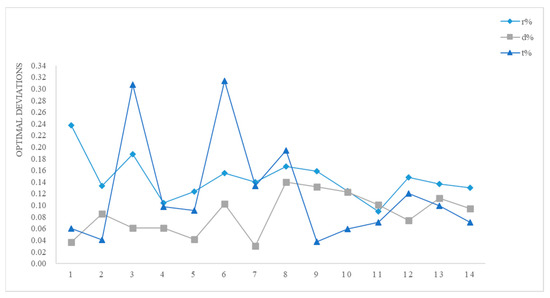
Figure 6.
Trend of Optimal Deviation.
As shown in Figure 6, the trend of the line shows that the optimal deviation is basically below 0.30. The solution stability of the route length works best, with r below 0.1 for most of the cases, and the upward and downward fluctuation is small. The number of vehicles is the next most stable solution, and the r of all the results remains at a low level except for the first set of cases. The optimal deviation values of the running time fluctuate widely, with higher t for the third, sixth, and eighth sets of cases, while the rest of the sets remain around 0.10. It is found that the size of the customers does not have a significant impact on the stability of the solution, and the optimal deviations of the three indicators are kept at the average level for the largest cases in groups 5 and 10. Therefore, the influence of different customer sizes on the computational stability of the solution method is small, and it is more due to the fluctuation of the results of each experiment caused by chance factors. In order to verify the solution effect of the balanced loading constraint method introduced in this paper, 1L-VRPSPD and 3L-VRPSPD are selected for comparison, and the optimal distance, number of vehicles and running time results obtained on the standard data set are compared as shown in Figure 7, Figure 8 and Figure 9. In order to express the advantage of the results obtained after the introduction of the balanced loading constraint more intuitively, the overall trend of GAP is shown in Figure 10.
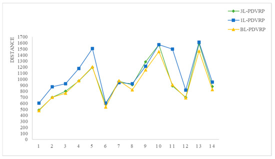
Figure 7.
Comparison of route lengths.
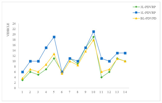
Figure 8.
Comparison of the number of vehicles.
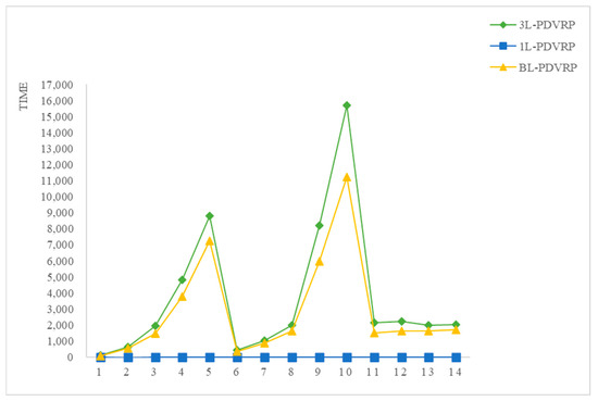
Figure 9.
Comparison of running times.
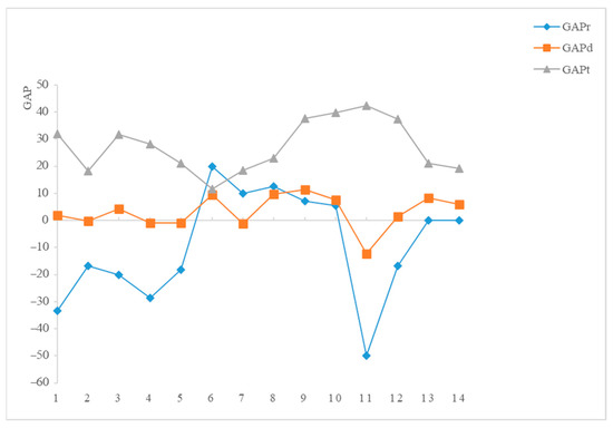
Figure 10.
Trend of GAP.
Analyzing the trend of the line graph presented in Figure 7 shows that 1L-VRPSPD has the largest route length, which is generally higher than the other two types of problems. In some cases, BL-VRPSPD achieves a shorter route length, indicating that the introduction of the balanced loading constraint does not compromise the effectiveness of the routing optimization.
As shown in Figure 8, among the 14 sets of calculation results, the results of the number of vehicles obtained from the 3L-PDVRPSPD and BL-PDVRPSPD problems do not differ significantly and are smaller than the results of the 1L-PDVRPSPD problem. In some of the cases, the number of vehicles obtained from the solution of the BL-VRPSPD problem is larger than that of the 3L-VRPSPD, which indicates that the introduction of the balanced loading constraint has a certain impact on the number of vehicles applied, and the main reason is that the introduction of the balanced loading constraint severely restricts the loading position of the goods, resulting in an increase in the number of vehicles.
As shown in Figure 9, the solution time for 1L-VRPSPD is much shorter than the other two types of problems, and the resulting solution time is not of the same order of magnitude. This indicates that the inclusion of the 3D loading constraint into the routing check session increases the number of iterations of the algorithm and substantially increases the solution time. In most of the cases, the solution times of BL-VRPSPD and 3L-VRPSPD are close to each other, and the solution efficiency of BL-VRPSPD is higher in the 5th, 9th, and 10th sets of cases. It shows that the introduction of balanced loading does not reduce the solution efficiency of the method, and the solution time decreases in large-scale cases, indicating that the solution efficiency of the proposed method becomes more obvious as the size of the customers increases.
As shown in Figure 10, in the 14 sets of results, the GAPd of route length basically lies above the 0-axis, the GAPr value curve of the vehicle number fluctuates more, and the GAPt of the running time lies above the 0-axis. Therefore, the introduction of the equilibrium loading constraint results in better pathfinding and has the same advantage in the solution efficiency.
In order to better verify the MOMD algorithm proposed in this paper, the advantages of the results of the total distance, number of vehicles and solution time obtained under the three different loading algorithms are analyzed and represented by bar graphs in Figure 11, Figure 12 and Figure 13.
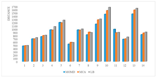
Figure 11.
Comparison of route lengths of different loading algorithms.
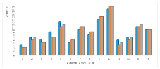
Figure 12.
Comparison of the number of vehicles with different loading algorithms.
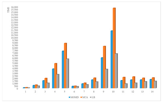
Figure 13.
Comparison of the running time of different loading algorithms.
As shown in Figure 11, MOMD achieves the best degree of routing optimization among the three algorithms in most cases. As shown in Figure 12, MOMD achieves a lower number of vehicles in some cases. As shown in Figure 13, in most cases, LB has the highest solution efficiency, mainly because LB does not perform multiple combinations, so it takes less time, while both MOMD and MCA algorithms consume more time in finding the optimal combination of loading space and goods, and the solution efficiency of MOMD is better in the comparison of these two algorithms, and the advantage is more prominent in large-scale cases.
6. Conclusions
For the demand of cost reduction and efficiency improvement faced by actual logistics and distribution, as well as the need to improve the safety of goods transportation, this paper proposes 3BL-VRPSPD, which optimizes the combination of goods-loading layout and pickup and delivery vehicle routing by considering 3D balanced loading. It is a realistic guide for improving the stability of the goods transportation process while enhancing the timeliness of logistics distribution and controlling the logistics cost in the specific pickup and delivery vehicle routing planning.
In this paper, we analyze the constraints at both vehicle routing and goods loading levels. Constraints, such as node access order, avoidance of sub-circuit, travel mileage limit, goods first-in last-out, support surface and balanced loading, are introduced. With the shortest total route length as the optimization objective, a 3BL-VRPSPD optimization model is constructed to portray the logistics distribution problem in a practical application scenario.
A hybrid heuristic algorithm with an improved TS as the optimization framework is proposed, an insertion heuristic algorithm is designed to construct the initial solution, and a loading algorithm MOMD is designed. The routing optimization is carried out by TS, and four independent parallel neighborhood operators are designed for neighborhood iterative transformations to find the optimization, while the loading layout is incorporated into the test link, and the feasibility judgment of the 3D balanced loading is integrated into the routing optimization process. Thus, we propose the optimization algorithm TS-MOMD.
This paper utilizes JAVA to implement the algorithm and selects standard cases as the dataset for analysis. The solution stability and efficiency of this algorithm are shown, and the results are compared with the existing algorithm, and the results show that the method still has a strong routing finding ability by adding the 3D balanced loading constraint.
The 3BL-VRPSPD is studied, and certain results are achieved, however, the problem is complex because it combines two NP-hard problems. The study still has some shortcomings and needs continuous improvement:
(i) In order to facilitate the study of the equilibrium loading constraint, only a single vehicle field and no time window are considered in the path. Subsequent studies can gradually consider adding constraints such as multi-vehicle yards and time windows to bring the problem closer to the actual situation.
(ii) The TS is used to find routing and a nested balanced loading algorithm, which requires a large number of traversals during routing optimization, making the number of iterations increase and the running time increase. In some cases, the solution time is high, which indicates that the algorithm can be greatly improved. Later on, we can develop a bootstrap algorithm to speed up the algorithm iteration process and a better loading algorithm to obtain a better loading solution.
Author Contributions
Conceptualization, Y.Z. and L.S.; methodology, Y.Z. and L.S.; software, L.S.; validation, Y.Z. and L.S.; formal analysis, Y.Z. and L.S.; resources, Y.Z. and L.S.; writing original draft preparation, L.S.; writing—review and editing, Y.Z. and L.S.; visualization, Y.Z. and L.S.; supervision, Y.Z.; project administration, Y.Z.; funding acquisition, Y.Z. All authors have read and agreed to the published version of the manuscript.
Funding
This work was supported by National Natural Science Foundation of China under Grant 71971220; Natural Science Foundation of Hunan Province 2023JJ30710 and 2022JJ31020.
Institutional Review Board Statement
Not applicable.
Informed Consent Statement
Not applicable.
Data Availability Statement
Not applicable.
Acknowledgments
This research is supported by the Central South University.
Conflicts of Interest
The authors declare no conflict of interest.
References
- Kovács, G. Methods for Efficiency Improvement of Produce and Logistic Processes. Res. Pap. Fac. Mater. Sci. Technol. Slovak Univ. Technol. 2018, 26, 55–61. [Google Scholar]
- Yongbo, W. Strategy and Path Analysis of Logistics Cost Reduction and Efficiency Improvement. Int. Workshop Adv. Soc. Sci. 2019, 62, 423–425. [Google Scholar]
- Chekoubi, Z.; Trabelsi, W.; Sauer, N.; Majdouline, I. The Integrated Production-Inventory-Routing Problem with Reverse Logistics and Remanufacturing: A Two-Phase Decomposition Heuristic. Sustainability 2022, 14, 13563. [Google Scholar] [CrossRef]
- Peng, D.; Zhao, Z.; Wu, G.; Boriboonsomsin, K. Bi-Level Fleet Dispatching Strategy for Battery-Electric Trucks: A Real-World Case Study. Sustainability 2023, 15, 925. [Google Scholar] [CrossRef]
- Dantzig, G.B.; Ramser, J.H. The Truck Dispatching Problem. Manag. Sci. 1959, 6, 80–91. [Google Scholar] [CrossRef]
- Krebs, C.; Ehmke, J.F.; Koch, H. Advanced loading constraints for 3D vehicle routing problems. OR Spectr. 2021, 43, 835–875. [Google Scholar] [CrossRef]
- Liu, Y.; Yue, Z.; Wang, Y.; Wang, H. Logistics Distribution Vehicle Routing Problem with Time Window under Pallet 3D Loading Constraint. Sustainability 2023, 15, 3594. [Google Scholar] [CrossRef]
- Guo, Q.E.; Wang, N.M. The Vehicle Routing Problem with Simultaneous Pickup and Delivery Considering the Total Number of Collected Goods. Mathematics 2023, 11, 311. [Google Scholar] [CrossRef]
- Koloch, G.; Kaminski, B.; Ao, S.I.; Katagir, H.; Xu, L.; Chan, H.S. Vehicle routing with three-dimensional container loading constraints—Comparison of nested and joint algorithms. In Proceedings of the International MultiConference of Engineers and Computer Scientists 2009, Hong Kong, China, 17–19 March 2010; pp. 145–157. [Google Scholar]
- Hu, H.; Li, X.; Zhang, Y.Y.; Shang, C.J.; Zhang, S.C. Multi-objective location-routing model for hazardous material logistics with traffic restriction constraint in inter-city roads. Comput. Ind. Eng. 2019, 128, 861–876. [Google Scholar] [CrossRef]
- Escobar-Falcón, L.; Alvarez-Martinez, D.; Wilmer-Escobar, J.; Granada-Echeverri, M. A specialized genetic algorithm for the fuel consumption heterogeneous fleet vehicle routing problem with bidimensional packing constraints. Int. J. Ind. Eng. Comput. 2021, 12, 191–204. [Google Scholar] [CrossRef]
- Gao, J.; Zheng, X.J.; Gao, F.; Tong, X.Y.; Han, Q.M. Heterogeneous Multitype Fleet Green Vehicle Path Planning of Automated Guided Vehicle with Time Windows in Flexible Manufacturing System. Machines 2022, 10, 197. [Google Scholar] [CrossRef]
- Yan, T.; Lu, F.; Wang, S. A hybrid metaheuristic algorithm for the multi-objective location-routing problem in the early post-disaster stage. J. Ind. Manag. Optim. 2023, 19, 4663–4691. [Google Scholar] [CrossRef]
- Wang, Z.; Wang, Y.; Jiao, Y. Uncertain Multi-Objective Hazardous Materials Transport Route Planning Considering Resilience and Low-Carbon. IEEE Access 2023, 11, 26921–26931. [Google Scholar] [CrossRef]
- Lu, F.Q.; Feng, W.J.; Gao, M.Y.; Bi, H.L.; Wang, S.X. The Fourth-Party Logistics Routing Problem Using Ant Colony System-Improved Grey Wolf Optimization. J. Adv. Transp. 2020, 2020, 8831746. [Google Scholar] [CrossRef]
- Abbaspour, S.; Aghsami, A.; Jolai, F.; Yazdani, M. An integrated queueing-inventory-routing problem in a green dual-channel supply chain considering pricing and delivery period: A case study of construction material supplier. J. Comput. Des. Eng. 2022, 9, 1917–1951. [Google Scholar] [CrossRef]
- Min, H. The multiple vehicle routing problem with simultaneous delivery and pick-up points. Transp. Res. Part A Gen. 1989, 23, 377–386. [Google Scholar] [CrossRef]
- Angelelli, E.; Mansini, R. The Vehicle Routing Problem with Time Windows and Simultaneous Pick-up and Delivery. Numer. Algorithms 2002, 519, 249–267. [Google Scholar]
- Liu, S.C.; Tang, K.; Yao, X. Memetic search for vehicle routing with simultaneous pickup-delivery and time windows. Swarm Evol. Comput. 2021, 66, 100927. [Google Scholar] [CrossRef]
- Jin, H.; Li, J.Q. A hybrid complementary metaheuristic for VRPTW with product classification and pickup-delivery constraints. J. Intell. Fuzzy Syst. 2023, 44, 1305–1322. [Google Scholar] [CrossRef]
- Avci, M.; Topaloglu, S. A hybrid metaheuristic algorithm for heterogeneous vehicle routing problem with simultaneous pickup and delivery. Expert Syst. Appl. 2016, 53, 160–171. [Google Scholar] [CrossRef]
- Nepomuceno, N.; Saboia, R.B.; Pinheiro, P.R. A Fast Randomized Algorithm for the Heterogeneous Vehicle Routing Problem with Simultaneous Pickup and Delivery. Algorithms 2019, 12, 158. [Google Scholar] [CrossRef]
- Li, J.; Guo, H.; Zhou, Q.; Yang, B. Vehicle Routing and Scheduling Optimization of Ship Steel Distribution Center under Green Shipbuilding Mode. Sustainability 2019, 11, 4248. [Google Scholar] [CrossRef]
- Qiu, F.; Zhang, G.; Chen, P.K.; Wang, C.; Pan, Y.; Sheng, X.; Kong, D. A Novel Multi-Objective Model for the Cold Chain Logistics Considering Multiple Effects. Sustainability 2020, 12, 8068. [Google Scholar] [CrossRef]
- Hou, L.; Hong, Z.; Zhao, J. A Novel Discrete Differential Evolution Algorithm for Stochastic VRPSPD. J. Comput. Inf. Syst. 2010, 6, 2227–2230. [Google Scholar]
- Tao, Z.; Chaovalitwongse, W.A.; Zhang, Y. Scatter search for the stochastic travel-time vehicle routing problem with simultaneous pick-ups and deliveries. Comput. Oper. Res. 2012, 39, 2277–2290. [Google Scholar]
- Subramanian, A.; Uchoa, E.; Pessoa, A.A.; Ochi, L.S. Branch-and-cut with lazy separation for the vehicle routing problem with simultaneous pickup and delivery. Oper. Res. Lett. 2011, 39, 338–341. [Google Scholar] [CrossRef]
- Subramanian, A.; Uchoa, E.; Pessoa, A. Branch-cut-and-price for the vehicle routing problem with simultaneous pickup and delivery. Optim. Lett. 2013, 7, 1569–1581. [Google Scholar] [CrossRef]
- Dethloff, J. Vehicle routing and reverse logistics: The vehicle routing problem with simultaneous delivery and pick-up. OR-Spektrum 2001, 23, 79–96. [Google Scholar] [CrossRef]
- Kalayci, C.B.; Kaya, C. An ant colony system empowered variable neighborhood search algorithm for the vehicle routing problem with simultaneous pickup and delivery. Expert Syst. Appl. 2016, 66, 163–175. [Google Scholar] [CrossRef]
- Zhang, W.Y.; Chen, Z.X.; Zhang, S.; Cai, Y.S. Dynamic multi-stage failure-specific cooperative recourse strategy for logistics with simultaneous pickup and delivery. Soft Comput. 2021, 25, 3795–3812. [Google Scholar] [CrossRef]
- Oztas, T.; Tus, A. A hybrid metaheuristic algorithm based on iterated local search for vehicle routing problem with simultaneous pickup and delivery. Expert Syst. Appl. 2022, 202, 117401. [Google Scholar] [CrossRef]
- Yu, V.F.; Aloina, G.; Jodiawan, P.; Gunawan, A.; Huang, T.C. The vehicle routing problem with simultaneous pickup and delivery and occasional drivers. Expert Syst. Appl. 2023, 214, 119118. [Google Scholar] [CrossRef]
- Salhi, S.; Nagy, G. Cluster insertion heuristic for single and multiple depot vehicle routing problems with backhauling. J. Oper. Res. Soc. 1999, 50, 1034–1042. [Google Scholar] [CrossRef]
- Peng, Z.S. Simultaneous delivery and pickup vehicle routing problem with three-dimension loading constraints. Comput. Eng. Appl. 2016, 052, 242–247. [Google Scholar]
Disclaimer/Publisher’s Note: The statements, opinions and data contained in all publications are solely those of the individual author(s) and contributor(s) and not of MDPI and/or the editor(s). MDPI and/or the editor(s) disclaim responsibility for any injury to people or property resulting from any ideas, methods, instructions or products referred to in the content. |
© 2023 by the authors. Licensee MDPI, Basel, Switzerland. This article is an open access article distributed under the terms and conditions of the Creative Commons Attribution (CC BY) license (https://creativecommons.org/licenses/by/4.0/).