Self-Paced Ensemble-SHAP Approach for the Classification and Interpretation of Crash Severity in Work Zone Areas

Abstract

The identification of causative factors and implementation of measures to mitigate work zone crashes can significantly improve overall road safety. This study introduces a Self-Paced Ensemble (SPE) framework, which is utilized in conjunction with the Shapley additive explanations (SHAP) interpretation system, to predict and interpret the severity of work-zone-related crashes. The proposed methodology is an ensemble learning approach that aims to mitigate the issue of imbalanced classification in datasets of significant magnitude. The proposed solution provides an intuitive way to tackle issues related to imbalanced classes, demonstrating remarkable computational efficacy, praiseworthy accuracy, and extensive adaptability to various machine learning models. The study employed work zone crash data from the state of New Jersey spanning a period of two years (2017 and 2018) to train and evaluate the model. The study compared the prediction outcomes of the SPE model with various tree-based machine learning models, such as Light Gradient Boosting Machine, adaptive boosting, and classification and regression tree, along with binary logistic regression. The performance of the SPE model was superior to that of tree-based machine learning models and binary logistic regression. According to the SHAP interpretation, the variables that exhibited the highest degree of influence were crash type, road system, and road median type. According to the model, on highways with barrier-type medians, it is expected that crashes that happen in the same direction and those that happen at a right angle will be the most severe crashes. Additionally, this study found that severe injuries were more likely to result from work zone crashes that happened at night on state highways with localized street lighting.

1. Introduction

Construction, preventative maintenance, and rehabilitation activities in work zones are essential for global highway maintenance and improvement. However, these actions change how traffic moves and raise the possibility of accidents. Due to changing traffic, reduced right-of-way, and road construction, work zones can lead to accidents [1]. In 2015, a construction zone accident occurred every 5.4 min in the United States [2]. Thus, drivers, traffic authorities, and experts are concerned about the crash risk in work zones [3]. Through enhanced work zone design based on association studies, highway authorities seek to reduce work zone crash risks [4,5].

Road safety analysis has focused on developing safety rules and preventative measures, sharing data about crash processes, and evaluating the relationship between crash or injury severity and contributing risk factors. The researchers have intended to ascertain the association between injury severity and crash risk variables including road alignment (geometry), driver qualities, vehicle features, seasonal influence, kind of crash, traffic rules, environmental conditions, and temporal factors. Road crash injuries have been evaluated using a variety of statistical techniques. The earlier studies used a variety of statistical models to predict and analyze the severity of road traffic injury, including generalized linear and non-linear models [6]; the weighted Poisson regression model (WPRM) [7]; mixed logit model (MLM) [8]; the ordered probit model (OPM) [9]; and the Bayesian approach to ordered probit [10].

Numerous studies have examined work-zone-related crash risk variables using historical crash data. Roadway alignment, the number of lanes, lighting, weather, weekday, and speed limit were found to impact the injury risk in work-zone-related crashes [11]. Vehicle and human-specific variables affect severe injury risk in work zones as well. According to Weng et al., [12], demographics of drivers and passengers, the use of airbags, their seat position, and the age of the vehicle can affect severe injuries in crashes related to work zones. The driver’s risk of injury depends on the work zone’s characteristics, such as construction activity, layout of the site, roadwork type (maintenance, construction, utility repair, etc.), and work zone length. The driver’s behavior in the work zone also affects crash risk: the driver’s choice of speed, stopping behavior, and trajectory may influence crash risk in different configurations/layouts of work zones. A driving simulator study linked a shorter taper length and a leading vehicle to higher accident risk in work zones. The vehicle type, speed, and inter-vehicle gaps all play a role. Reducing approach distance from a work zone increases rear-end collision risk. Therefore, lane merging should occur further upstream, prior to the location of the work zone [13].

Concerns have also been raised about the impact of speed limit violations and fast-moving vehicles on work zone safety [14]. According to these studies, there is a direct relationship between platoon characteristics, timing, traffic volume, and other vehicle compliance and drivers’ speeding behavior in construction zones. According to speed data gathered over time, the leading vehicle of a platoon with a greater distance was more likely to accelerate. Regardless of the posted temporary speed limits, some drivers would drive through a work zone at speeds corresponding to their perceptions of the traffic conditions and speed environment. As a result, there would be a major difference in speeds between the speed-limit-compliant and non-compliant drivers [15].

The impact of truck traffic on work zone crashes has also been studied. The studies indicate an association between increased severity of work zone crashes and the involvement of trucks in the crashes [16]. The truck indicator served as a binary explanatory variable in the injury severity model of Li and Bai [17]. The association between injury severity and various risk variables in large truck crashes in Minnesota between 2003 and 2012 was examined by Osman et al. [18] using several statistical models. In truck-related collisions, the authors noticed significant variations in the severity of injuries between rural and urban functional road classes. Statistical models may have clearly defined functional forms, but they frequently call for rigor in the model assumptions about how different variables interact. As a result, the estimation outputs of the models may be biased or inaccurate if their implicit assumptions are compromised. In addition, contemporary data sources often generate intricate, multidimensional data sets that are challenging to model using conventional statistical models. On the contrary, machine learning (ML) models are extremely adaptable and require few or no assumptions [19]. Thus, it is no surprise ML modelling has become one of the most popular and feasible approaches for the estimation of injury severity in road crashes [20,21]. In healthcare research [22] and financial research [23], ML models have also been extensively employed.

While superior diagnostic skills are necessary for ML models, it is more essential to comprehend how crashes occur in work zones. This is particularly important in identifying and formulating mitigation strategies for crash prevention in work zones. However, the “black box” nature of most ML models is a critical limitation. Sensitivity analysis techniques have been combined with ML models in road safety studies to interpret the effects of various risk factors on the severity of injuries. Interpretability can be divided into two distinct categories: global interpretability, which explains the model’s behavior across the dataset, and local interpretability, which explains a particular prediction. Partial dependency plots (PDP), accumulated local effects (ALE), and local interpretable model-agnostic explanation (LIME) are the methods for ML model interpretation. However, the assumption of independence and instability of the explanations by these methods may result in inaccurate estimations of safety effects in traffic safety studies. Recently, numerous researchers have employed the Shapley additive explanations (SHAP) technique to address this issue [24]. Using the Shapley value, this technique, based on the game theory approach and local explanations, can explain the relationship between the input variables and the decision factor. SHAP analysis has been widely integrated with ML models in traffic safety research [25,26].

Furthermore, addressing class imbalance is crucial to predicting the injury severity of crashes in work zones. The injury class, which includes fatal, major, and minor injuries, is typically much smaller than the property damage only (PDO) class. This imbalance has a negative impact on classification algorithms, as they frequently misclassify minority instances (injuries in our case) more often than majority instances (PDO). In extreme circumstances, ML models may incorrectly classify all instances as instances of the majority class, resulting in high precision for the majority class and unacceptably low precision for the minority class of interest. Typically, three strategies are used to address the class-imbalance issue: a data-level approach, an algorithm-level approach, and an ensemble strategy. The data-level strategy focuses on enriching the dataset to make it appropriate for training a prediction algorithm. This can be accomplished by balancing the dataset distribution, which can be categorized as either oversampling or under-sampling. In the oversampling technique, new instances from the minority class are synthesized using SMOTE, SMOTE-NC, ADAYSN, or ADAYSN-NC. In the under-sampling strategy, the number of majority class instances is decreased to match the instances in the minority class, such as the Near-Miss (NM) strategy. The algorithm-level strategies, such as cost-sensitive learning algorithms, augment existing models to reduce their majority-class bias.

Similarly, these strategies require a deeper understanding of the modified learning algorithm and a more thorough identification of the causes of the algorithm’s inability to learn representations for skewed distributions. The ensemble strategy combines an algorithm-level or a data-level method with an ensemble learning technique to produce a dependable and precise classification model. Due to their superior performance on imbalanced data, the ensemble strategies are acquiring popularity in many real-world applications such as SMOTEBoost [27], which combines SMOTE and an adaptive boosting model. Other ensemble strategies use a different classifier as their base learner; for example, EasyEnsemble [17] uses several AdaBoost models to develop a robust ensemble. However, due to the presence of algorithm-level and data-level imbalance learning strategies in their pipeline, when applied to realistically imbalanced data, these ensemble approaches may suffer from poor applicability or low efficiency.

In order to solve this issue, Liu et al., [28] proposed a novel SPE model for imbalance classification that uses under-sampling and self-paced data harmonization to create a robust ensemble. This approach has produced robust performance in the presence of severely skewed distributions in addition to being computationally efficient. Therefore, in this study, the SPE model for the prediction and imbalance classification problem is proposed to improve the prediction performance of work zone crash injury severity. The suggested SPE is an ensemble learning strategy created to tackle the problem of severely imbalanced classification in huge datasets. The presented solution has remarkable computing efficiency, outstanding performance, and extensive compatibility with various learning models, and it provides an easy approach to class-imbalanced issues. The performance of the SPE model is then compared to the advanced tree-based ML models, with and without augmented data, including adaptive boosting (AdaBoost) + untreated data, AdaBoost + SMOTE-ENN treatment, Light Gradient Boosting Machine (LGBM) + untreated data, LGBM + SMOTE-ENN treatment, classification and regression tree (CART) + untreated data, and CART + SMOTE-ENN treatment as well as binary logistic regression (BLR) + untreated data and BLR + treated data. Furthermore, the SHAP technique has also been employed to ascertain the significance and contribution of numerous risk variables that affect work-zone-related crashes. Providing a novel approach for prediction (i.e., SPE) and assessing the importance of factors on work zone crash injury severity with the SHAP technique introduce a promising approach for safety in transportation.

The remainder of this paper has the following structure. The research methodology is presented in Section 2 along with a description of the data, a detailed description of the proposed SPE model, a description of the SMOTE-ENN technique, a description of tree-based ML models and BLR models, and a description of the SHAP interpretation system. Section 3 discusses the results of the SPE model and contrasts them with those of ML models and BLR models. The SPE results are used for SHAP analysis to interpret and explain the model. Lastly, Section 4 encapsulates the conclusions and outlines additional research recommendations.

2. Materials and Methods

Previously, tree-based ML models and Bayesian models were widely used to predict crash injury severity [20,21]. The crash dataset pertaining to work zones was subjected to preprocessing procedures to partition the data into distinct testing and training sets. An SPE model, tree-based ML models, and a BLR model were constructed using the training data set. The testing dataset measured the performance of the model. One advantage of the SPE model over the tree-based ML model could be justified in that during the pre-processing phase, the SPE paradigm does not necessitate data balance, which saves computational time and effort. However, before the commencement of training, it is necessary to ensure data balance for the tree-based machine learning models and the Bayesian linear regression model. The case study training dataset involved the application of SMOTE-ENN to work zone crash records sourced from the New Jersey Department of Transportation (NJDOT) crash records database for the period spanning 2017 to 2018. A subset of the training dataset was utilized to optimize the hyperparameters. Using a Bayesian optimization technique, the SPE model and tree-based ML models were optimized. The SPE model’s performance was evaluated and compared to the ML models and the BLR model. The SHAP interpretation system analyzed risk variables and their interplay in work zone accidents. Figure 1 depicts the operational paradigm of the study.

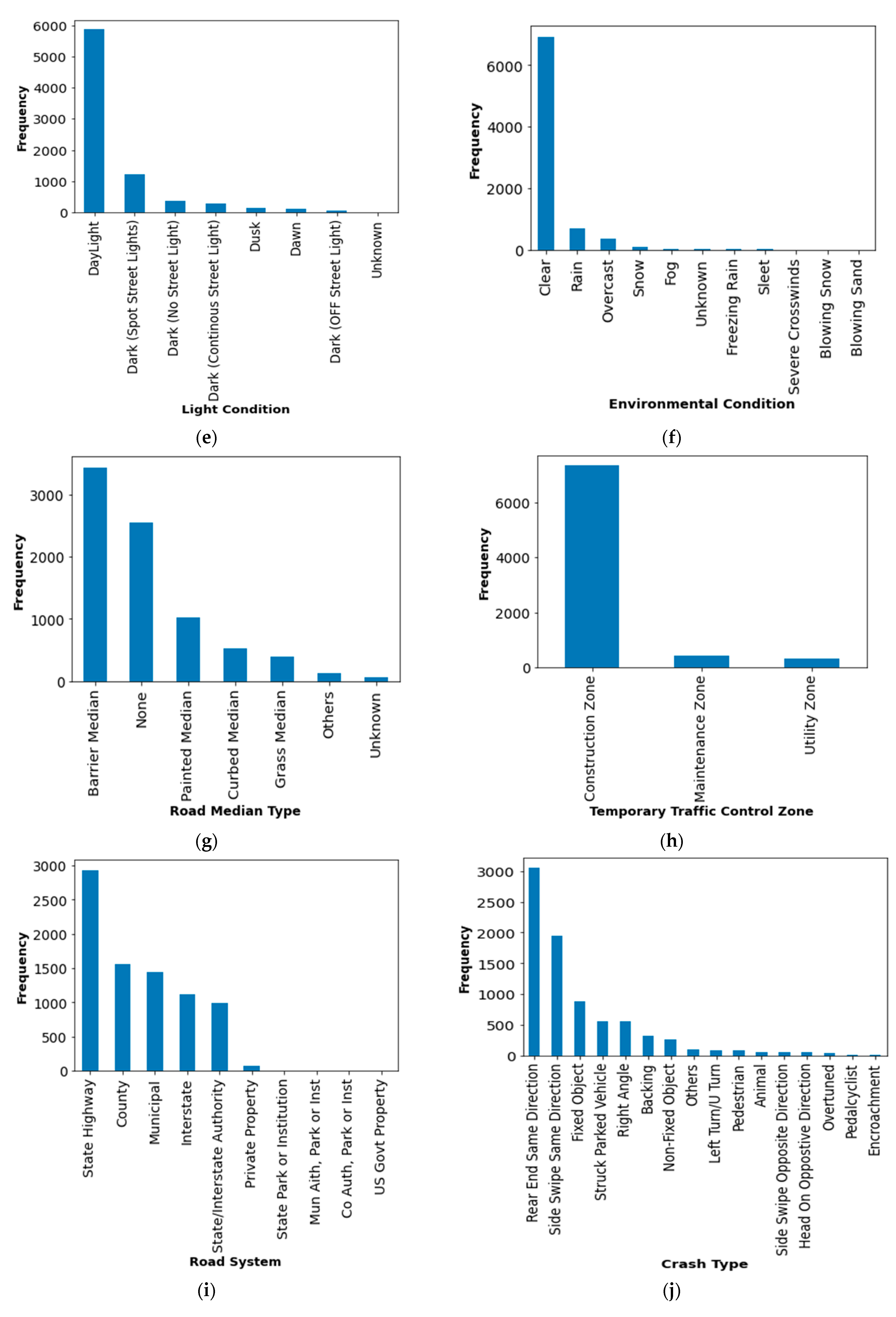
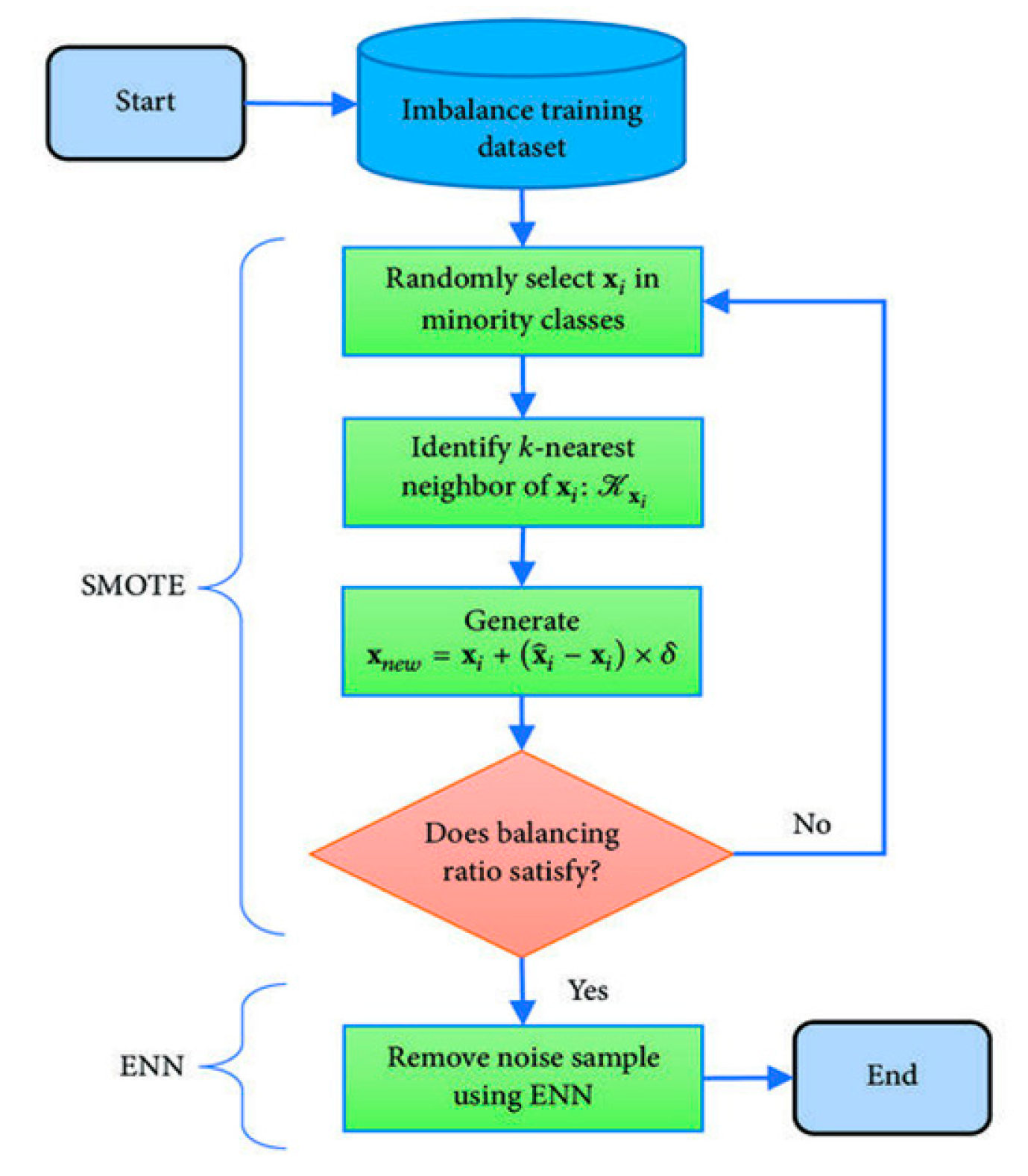
2.1. Data Description and Augmentation

The crash data in this study were obtained from the NJDOT crash records database, which is publicly accessible via the NJDOT website. The dataset contained records of 8102 crashes that happened in work zones in the state of New Jersey between 2017 and 2018. The crashes were divided into two categories based on the severity of crashes: PDO and injury. Injury included fatal, major (or incapacitating), and minor injuries. The crash risk variables used in this research were derived from the crash records and are listed in

Table 1. Coding of risk variables for the analysis.

Risk Variable	Codes and Description
Road Character–Road Horizontal Alignment	0: ‘Unknown’, 1: ‘Straight’, 2: ‘Curved Left’, 3: ‘Curved Right’,
Road Character–Road Grade	0: ‘Unknown’, 4: ‘Level’, 5: ‘Down Hill’, 6: ‘Up Hill’, 7: ‘Hill Crest’, 8: ‘Sag’
Road Surface Type	0: ‘Unknown’, 1: ‘Concrete’, 2: ‘Black Top’,3: ‘Gravel’, 4: ‘Steel Grid’, 5: ‘Dirt’, 6: ‘Others’
Road Surface Condition	0: ‘Unknown’, 1: ‘Dry’, 2: ‘Wet’, 3: ‘Snowy’, 4: ‘Icy’, 5: ‘Slush’, 6: ‘Standing Water’, 7: ‘Sand’, 8: ‘Oil’, 9: ‘Mud’, 10: “Others”
Light Condition	0: ‘Unknown’, 1: ‘Daylight’, 2: ‘Dawn’, 3: ‘Dusk’, 4: ‘Dark (Off Street Light)’, 5: ‘Dark (No Street Light)’, 6: ‘Dark (Spot Street Lights)’, 7: ‘Dark (Continuous Street Light)’
Environmental Condition	0: ‘Unknown’, 1: ‘Clear’, 2: ‘Rain’, 3: ‘Snow’, 4: ‘Fog’, 5: ‘Overcast’, 6: ‘Sleet’, 7: ‘Freezing Rain’,8: ‘Blowing Snow’, 9: ‘Blowing Sand’, 10: ‘Severe Crosswinds’
Road Median Type	0: ‘Unknown’, 1: ‘Barrier Median’, 2: ‘Curbed Median’, 3: ‘Grass Median’, 4: ‘Painted Median’, 5: ‘None’, 6: ‘Others’
Temporary Traffic Control Zone	2: ‘Construction Zone’, 3: ‘Maintenance Zone’, 4: ‘Utility Zone’
Crash Type	1: ‘Rear End Same Direction’, 2: ‘Side Swipe Same Direction’, 3: ‘Right Angle’, 4: ‘Head On Opposite Direction’, 5: ‘Side Swipe Opposite Direction’, 6: ‘Struck Parked Vehicle’, 7: ‘Left Turn/U Turn’, 8: ‘Backing’, 9: ‘Encroachment’, 10: ‘Overtuned’, 11: ‘Fixed Object’, 12: ‘Animal’, 13: ‘Pedestrian’, 14: ‘Pedalcyclist’, 15: ‘Non-Fixed Object’, 16: ‘Others’
Road System	1: ‘Interstate’, 2: ‘State Highway’, 3: ‘State/Interstate Authority’, 4: ‘State Park or Institution’, 5: ‘County’, 6: ‘Co Auth, Park or Inst’, 7: ‘Municipal’, 8: ‘Mun Aith, Park or Inst’, 9: ‘Private Property’, 10: ‘US Govt Property’
Type of Day	1: ‘Weekday’, 0: ‘Weekend’
Number of Vehicles Involved	1: ‘Multiple Vehicles’, 0: ‘Single Vehicle’

along with their respective codes and value descriptions. Figure 2 depicts the relative frequency distributions of the variables.

Notably, the dataset of work-zone-related crash records analyzed for this study was imbalanced regarding crash severity. From 1 January 2017 to 31 December 2018, there were 8102 crashes in work zones, including 10 fatalities (about 0.1 percent of the total), 1609 non-fatal injury crashes (about 20%), and 6473 PDO crashes. Due to the small number of fatal injuries within the sample, the fatal injuries and non-fatal injuries were analyzed as a single class. The category labeled “injury” comprised 1629 crash records or 20.10% of the total (see Figure 3).

Even with this data augmentation, there was a significant imbalance between the majority class (PDO crashes) and the minority class (injury crashes). Consequently, additional data augmentation was required in the preprocessing stage, before training the tree-based ML and BLR models. The data imbalance can be addressed by adjusting the distribution of instances among the classes, typically through a resampling procedure that generates more records in the minority classes. In this study, a hybrid SMOTE-ENN resampling method was applied. This method combines SMOTE and ENN in order to provide a more balanced dataset. First, the minority class in the original training dataset was over-sampled by creating synthetic examples in the variable space using each instance and its k-nearest neighbors. This was proceeded by the elimination of some data collected from the majority and minority classes that had a different class than the majority class of their k-nearest neighbor. Thus, the two-step SMOTE-ENN procedure is described as Figure 4.

2.2. Self-Paced Ensemble (SPE) Model for Imbalanced Crash Data

This study used a recently developed ensemble-based imbalance learning SPE approach [28] to develop a classification and prediction framework for the work-zone-related crash severity. This ensemble learning strategy aims to tackle the issue of imbalanced classification in datasets of considerable size. The proposed solution provides a user-friendly approach to tackle class imbalance issues, demonstrating remarkable computational efficacy, praiseworthy efficacy, and extensive adaptability to various learning models. We first introduce the concepts of hardness harmonization and self-paced factor before going into detail about the SPE approach.

2.2.1. Hardness Harmonize

The effort of correctly classifying an instance with a particular classifier is referred to as its hardness. In context of this, the classification hardness distribution provides an indication of the task’s difficulty. For example, noisy data are likely to have high levels of hardness. The data samples can be classified as trivial, noisy, or borderline based on their difficulty level. We employ the symbol $\left(\hslash \right)$ to indicate the classification hardness function, which can represent any decomposable error function. This means that the overall error is obtained by adding the errors from each sample, such as cross entropy, absolute error, and squared error.

Assuming $F_v$ is a classification model to be trained, we use $F_v\left(x\right)$ to represent the likelihood that $\mathit{x}$ is a positive instance in the output of the classifier. Then, the classification hardness of an instance $\left(x,y\right)$ wrt $F_v$ is denoted by the function $\hslash \left({x,y,F}_v\right)$. In this concept, all cases of the majority class label are partitioned into $k$ bins, where $k$ is a hyperparameter that is defined based on its hardness value. Each $k^{\mathit{th}}$ bin denotes a specific hardness level. The majority class label examples are then under-sampled in order to preserve the same overall hardness contribution in each bin and provide a balanced dataset. The term “harmonize” is used to describe this strategy in the literature on gradient-based optimization. This study used a similar approach to balance the hardness, but only in the first round. The main cause is that when the ensemble classification model gradually adapts to the training dataset, the quantity of trivial examples grows during training. Thus, simply adjusting the hardness impact results in many pointless samples. These less instructive examples greatly slow down later repetitions of the learning process. To overcome this issue, we do not only apply hardness harmonization in all rounds. Instead of this, “self-paced factors” were created to undertake self-paced harmonized under-sampling.

2.2.2. Self-Paced Factor

If selection is based on maintaining the same hardness, a large number of samples that fit the criteria will be retained, resulting in a classifier that lacks diversity. Consequently, a balancing factor is added to decrease the probability of certain samples during the iteration. After harmonizing the hardness contribution of each bin, the likelihood of an instance occurring in bins with a large initial population decreases progressively. A self-paced factor determines the rate of decline $\left(\mathbf{\sigma }\right)$. When $\mathbf{\sigma }$ is high, the tougher instances receive more attention than the simple hardness contribution harmonize. Outliers and noise have little effect on the model’s capacity to generalize in the initial few iterations since the model focuses on instructive borderline situations. When $\mathbf{\sigma }$ is quite large after several iterations, the model keeps a sufficient number of trivial instances as the “skeleton”, preventing over-fitting. Algorithm 1 below displays the SPE model’s pseudo code. It is important to note that the hardness value is modified after each iteration (lines 5–6) in order to choose the data instances that were the most useful for the current ensemble. The self-paced factor growth has been controlled by the tangent function (line 8). The self-paced factor equals 0 in the first iteration and 0 in the last iteration.

Algorithm 1: SPE model
Input: Hardness function $\left(\hslash \right)$, training data $M_e={\left\{\left(x_k{,y}_k\right)\right\}}_1^n$, base estimators $\left(\mathsf{\zeta }\right)$, number of base estimators $\left(\zeta \right)$, number or amount of bins $\left(k\right)$
	Initialize: $\mathsf{𝒫}$ is the minority class instances in $M_e$, $𝒩$ is the minority class instances $M_e$,
	The estimator ${\mathsf{\zeta }}_0$ is trained by employing randomly under-sampled majority subsets, ${𝒩}_o^{\prime }$ and $\mathsf{𝒫}$, where $\left|{𝒩}_o^{\prime }\right|=\left|\mathsf{𝒫}\right|$
	for $v=1 \mathrm{to} n$do
		Create ensemble of base estimators $F_v\left(x\right)=\frac{1}{v}{\displaystyle \sum _{j=0}^{v-1}{\mathsf{\zeta }}_j}\left(x\right)$
		Split the majority subset into $k$ bins w.r.t $\hslash \left({x,y,F}_v\right)$: $\left(b_1{,b}_2,\dots {,b}_{\xi }\right)$
		The mean hardness contribution in the $l^{\mathit{th}}$ bin is given as: $h_l={\displaystyle {\sum }_{s\in b_l}h}\left(x_s{,y}_s{,F}_v\right)/\left|b_l\right|, \forall l=1,2,\dots ,k$
		The self-paced factors is updated as $\mathbf{\sigma }=\mathit{tan}\left(\frac{i\mathsf{\Pi }}{2\zeta }\right)$
		Un-normalized sampling weight of the $l^{th}$ bin is: $p_l=\frac{1}{h_l+\mathsf{\sigma }},\forall l=1,2,\dots ,k$
		Under-sampling is performed from the $l^{th}$ bin with $\frac{p_l}{{\displaystyle {\sum }_m{p}_l}}\left|{\rm P}\right|$ instances
		Train the estimator ${\mathsf{\zeta }}_i$ by employing newly generated under-sampled set
	End
	Output Robust ensemble model $F\left(x\right)=\frac{1}{\xi }{\displaystyle \sum _{m=1}^{\xi }{\mathsf{\zeta }}_m}\left(x\right)$

2.3. Tree-Based ML Models

In addition to the SPE model, advanced tree-based ML models were applied in the study, including CART, LGBM, and AdaBoost. These models are briefly described herein.

2.3.1. Classification and Regression Tree (CART)

CART is a decision-tree learning method that uses the Gini index to categorize data (Steinberg and Colla, 2009). According to a decision rule, parent nodes in the tree are repeatedly divided in a binary manner, as shown in Figure 5, until all child nodes are homogeneous.

In order to tidy up the terminal nodes during the tree-growing process, the target variable must be partitioned repeatedly. The Gini Index is a gauge of a given node’s impurity in a tree, as illustrated in Equation (1). The dataset is more pure and the classification is more accurate when the Gini score is lower.

$$\mathrm{Gini}\left(\mathrm{X}\right)=1-{\displaystyle \sum {\mathit{\rho }}_{\mathrm{a}}^2}$$

(1)

In our study, $\mathrm{X}$ denotes the training dataset, ${\mathit{\rho }}_{\mathrm{a}}$ denotes the probability of appearing category $\mathit{a}$ in $\mathrm{X}$.

The CART keeps growing the tree until homogenous outcomes are attained. Pruning trees is therefore required to keep them from growing to be complex maximal trees. The classifier eliminates the branches that are not important to it. By cutting branches from the tallest trees, the process for pruning trees produces smaller, more straightforward trees. Equation (2) states that smaller trees have a larger misclassification error rate.

$$\mathrm{ER}={\displaystyle \sum {\mathit{\rho }}_{\mathrm{a}}\mathrm{Gini}\left(\mathrm{X}\right)}$$

(2)

2.3.2. Adaptive Boosting (AdaBoost)

Adaptive boosting is an iterative ensemble learning strategy. By combining numerous different classifiers, it develops a strong classifier. The core idea behind the AdaBoost method is to build weak classifier weights before training the model in each iteration to get (more) accurate estimations of the observations. As a base-classifier, you can use any ML technique that accepts weights from the training dataset. The following is a description of how AdaBoost operates in Algorithm 2 below:

Algorithm 2: Adaptive Boosting (AdaBoost)
	Input: Training dataset: $M_e={\left\{\left(x_k{,y}_k\right)\right\}}_1^n$, weak learner $h_t$
	Initialize the distribution of weight as ${\omega }_1(k)=\frac{1}{m}$
	for   $t=1 \mathrm{to} \mathrm{T}$ do
		By the utilization of weight distribution ${\omega }_t$, the weak learner is trained $h_t: \mathrm{{\rm X}}\to R$
		For $h_t$, determine the weight $\psi$
		Over the training data set, the weight distribution is updated. ${\omega }_{t+1}\left(k\right)=\frac{{\omega }_t\left(k\right){\exp }^{{-\psi }_t{Y}_k{h}_t\left({\mathrm{{\rm X}}}_k\right)}}{{\mathrm{\Omega }}_t}$ Here, ${\mathrm{\Omega }}_{\mathrm{t}}$ is a factor that is known as a normalization factor. It is chosen such that ${\omega }_{t+1}$ will be a distribution.
	End for
	Return $\mathbb{F}\left(\mathit{X}\right)={\displaystyle {\sum }_{t=1}^{\mathrm{𝒯}}{\psi }_t{h}_t\left(X\right) }$ as well as $\mathrm{H}\left(\mathit{X}\right)=\mathrm{sign}\left(\mathbb{F}\left(\mathrm{{\rm X}}\right)\right)$

2.3.3. Light Gradient Boosting Machine (LGBM)

Researchers from Peking University in China and Microsoft came up with the LGBM variant of the gradient boosting decision tree (GBDT) to address the performance and scalability issues present with the GBDT in situations involving high-dimensional input parameters and enormous volumes of data. In contrast to other methods, which divide the tree from level to level, this one uses methods based on decision trees to instead divide the tree from leaf to leaf. When developing on the same leaf, splitting in a leaf-wise direction rather than a level-wise direction minimizes loss more than splitting in a level-wise direction does. This results in much higher classification accuracy than most commonly used boosting strategies. The level-wise and leaf-wise expansion of the tree are depicted in Figure 6 for the purposes of LGBM and gradient boosting. The gradient-based one-sided sampling and the exclusive factor bundling (EFB) methods are the two separate strategies that LGBM uses.

2.3.4. Binary Logistic Regression (BLR)

In contrast to the ML models, the BLR is a statistical modelling technique in which relationships between a dichotomous or binary decision factor and one or more risk factors are modelled. The BLR uses explanatory risk factors to predict the probability of the binary decision factors taking one of the two binary values. In injury severity modelling, the logit is natural log of the odds that the dichotomous response value $y$ is injury $\left(y=1\right)$ versus PDO $\left(y=0\right)$, as illustrated by Equations (3) and (4).

$$\mathit{logit}\left(\rho \right)=\mathit{ln}\left(\frac{\rho }{1-\rho }\right)={\beta }_0{+\beta }_1{k}_1,\dots {,+\beta }_i{k}_i{+\epsilon }_i$$

(3)

$$\rho =\mathit{prob}\left({\mathit{y}}_i=1/X\right)$$

(4)

where,

$\rho$: likelihood of occurrence of injuries

$1-\rho$: likelihood of occurrence of PDO

$k_i$: $i^{\mathrm{th}}$ risk factor

${\beta }_i$: $i^{\mathrm{th}}$ coefficient of the BLR model

$X$: vector of risk factors

${\epsilon }_i$: random error term

The odds ratio (OR) of injury is the probability or likelihood of injury cases divided by the likelihood or probability of PDO cases. When any risk factor enhances the probability of an outcome by one unit, while the remaining risk factor values are kept unchanged, the odds rise by an amount $\mathit{exp}\left({\beta }_i\right)$.

2.4. Hyperparameter Tuning

Hyperparameter tuning is necessary prior to training the ML models. This lessens complexity, prevents over-fitting, and enhances the learning method. The performance metric used in this study for hyperparameter adjustment was G-Mean. Grid search cross-validation (GS-CV), random search cross-validation (RS-CV), and Bayesian optimization technique (BOT) are a few of the methods for hyperparameter tuning that have been discussed in the literature [29,30,31]. For example, grid search cross-validation and random search cross-validation iteratively scan the whole space of potential hyperparameter values without taking into account prior results.

Nonetheless, based on earlier evaluations, the Bayesian optimization approach chooses the following set of hyperparameters. It can concentrate on the parameters that result in higher validation results by cleverly mixing the parameters. Finding the ideal hyperparameter values with this method takes fewer iterations.

2.5. Model Evaluation

The performance of the SPE and tree-based ML models and the BLR model can be evaluated by a number of metrics generally derived from the model’s contingency or confusion matrix, depicted in Figure 7.

Results are considered to be true positives $\left({\Delta }^{\mathit{\rho }}\right)$ when the classifier accurately predicts the positive class for those results. In the same vein, true negatives $\left({\Delta }^{\mathit{\eta }}\right)$ are the results for which the classifier makes a correct prediction regarding the absence of a given class. When a model mistakenly predicts the presence of a positive class, this is known as a false positive $\left({\nabla }^{\mathit{\rho }}\right)$. In a similar vein, false negatives $\left({\nabla }^{\mathit{\eta }}\right)$ are the outcomes that occur when the classifier makes an inaccurate prediction regarding the negative class.

The overall classification accuracy is a common model performance indicator that can be calculated as the ratio of the total number of correct predictions to the total number of predictions. This metric has the potential to yield erroneous conclusions in the case of unbalanced data sets since it gives more weight to the more numerous class. Under these conditions, the precision of classification cannot be utilized as a performance metric. To solve this problem, in addition to accuracy, a number of other performance indicators, including precision, recall, geometric mean (G-Mean), and Matthews’ correlation coefficient, are utilized (MCC). The expressions for each performance statistic may be found in (5) through (9) below. G-Mean is a performance statistic that illustrates the equilibrium between the classification performances of minority (e.g., injury) and majority (e.g., PDO) cases. It does this by comparing the percentage of examples that fall into each category. A classification algorithm that was trained on unbalanced data can benefit from using the MCC, which is an additional helpful statistic for evaluating the algorithm’s effectiveness. The values of MCC should fall somewhere in the range of −1 to 1. A higher level of performance is represented by values that are closer to +1, and vice versa.

$$\mathit{Classification} \mathit{Accuracy}=\frac{{\Delta }^{\mathit{\rho }}+{\Delta }^{\mathit{\eta }}}{{\Delta }^{\mathit{\rho }}+{\Delta }^{\mathit{\eta }}+{\nabla }^{\mathit{\eta }}+{\nabla }^{\mathit{\rho }}}$$

(5)

$$\mathit{Precision}=\frac{{\Delta }^{\mathit{\rho }}}{{\Delta }^{\mathit{\rho }}+{\nabla }^{\mathit{\rho }}}$$

(6)

$$\mathit{Recall} \mathit{or} \mathit{TPR}=\frac{{\Delta }^{\mathit{\rho }}}{{\Delta }^{\mathit{\rho }}+{\nabla }^{\mathit{\eta }}}$$

(7)

$$G-\mathit{Mean}=\sqrt{\left(\frac{{\Delta }^{\mathit{\rho }}}{{\Delta }^{\mathit{\rho }}+{\nabla }^{\mathit{\eta }}}\right)\left(\frac{{\Delta }^{\mathit{\eta }}}{{\nabla }^{\mathit{\rho }}+{\Delta }^{\mathit{\eta }}}\right)}$$

(8)

$$\mathit{MCC}=\frac{{\Delta }^{\mathit{\rho }}\times {\Delta }^{\mathit{\eta }}-{\nabla }^{\mathit{\rho }}\times {\nabla }^{\mathit{\eta }}}{\sqrt{\left({\Delta }^{\mathit{\rho }}+{\nabla }^{\mathit{\rho }}\right)\left({\Delta }^{\mathit{\rho }}+{\nabla }^{{}^{\mathit{\eta }}}\right)\left({\Delta }^{{}^{\mathit{\eta }}}+{\nabla }^{\mathit{\rho }}\right)\left({\Delta }^{{}^{\mathit{\eta }}}+{\nabla }^{{}^{\mathit{\eta }}}\right)}}$$

(9)

2.6. SHAP Interpretation

Lundberg and Lee [24] devised a tool for conducting SHAP (Shapley additive explanations) analysis, which utilizes game theory principles to enhance users’ comprehension of machine learning (ML) models. The purpose was to enhance the transparency and interpretability of machine learning models. The SHAP analysis offers two notable benefits. The first is global interpretability, whereby the SHAP values can effectively demonstrate the extent to which each predictor positively or negatively contributes to the target variable. Second, local interpretability is achieved through the provision of a unique set of SHAP values for each observation. While ML models are being trained or tested, a prediction value is generated for each instance, and the SHAP value corresponds to the value that is assigned to each instance’s components. This applies whether the model is being trained or tested. Using the equation, one may determine the contribution made by each factor, which is denoted by the Shapley value (10).

$${\phi }_i={\displaystyle \sum _{\Upsilon \subseteq \Pi \left\{i\right\}}\frac{\Upsilon !\left(n - \left|\Upsilon \right| - 1\right)!}{n!}}\left[f\left(\Upsilon \cup \left\{i\right\}\right) - f\left(\Upsilon \right)\right]$$

(10)

where ${\phi }_i$ represents the role of the $i^{\mathrm{th}}$ factor, $\Pi$ represents the set of all factors, $\Upsilon$ represents the subset of the given predicted factor, and $f\left({\Upsilon }_i\right)$ and $f\left(\Upsilon \right)$ represent the model results with and without $i^{\mathrm{th}}$ factors, respectively. The SHAP analysis tool uses an additive factors imputation technique to create an interpretable machine learning model, where the output model is defined as the linear sum of the input factors (Equation (11)).

$$g\left(z\prime \right){=\phi }_0+{\displaystyle \sum _{i=1}^{\Lambda }{\phi }_i}z\prime$$

(11)

Here, $z\prime \in {\left\{0,1\right\}}^{\Lambda }$ when a factor is observed = 1; otherwise = 0. $\Lambda$ denotes the number of input factors, ${\phi }_0$ is the base values, i.e., the predicted outcome without factors, and ${\phi }_i$ represents the Shapley value of $i^{\mathrm{th}}$ risk factor. The SPE model and the major factors that are likely to cause injuries in work-zone-related crashes were analyzed using the SHAP model in this study. The study was conducted in the United Kingdom. In addition, factor interaction analysis was performed with the SHAP tool.

3. Results

This study utilized an effective new SPE model, tree-based ML models, and a BLR model to forecast the severity of crashes associated with work zones. This study employed Python 3.6, an open-source and free programming language, for model development and testing. The models were developed and assessed using sklearn.metrics, imbeans, sklearn.ensemble, scikit-learn, sklearn.metrics, and shap Python libraries. For the purposes of developing the SPE model, the ML models, and the BLR model, the dataset, including 8102 crash records, was partitioned into three subsets as follows: 70% of the data, which totaled 5672 crash reports, was partitioned into training and validation sets, while only 30% of the data, which totaled 2433 crash records, was used for testing. When the models were built with the help of the training set, the validation data set was used to adjust the hyperparameters of the models and make them as accurate as possible. In order to establish the ideal hyperparameters for the tree-based ML models as well as the SPE model, Bayesian optimization was utilized. The results of this endeavor are provided in

Table 2. Hyperparameter tuning of model parameters.

Treatment	Model	Hyperparameters	Range	Optimal Values
No treatment	SPE	Number of trees	[100–3000]	949
		Max depth	[0–10]	6
		Learning rate	[0.01–0.1]	0.056
	LGBM	Number of trees	[100–3000]	2466
		Learning rate	[0.01–0.5]	0.081
		Max depth	[0–10]	7
		Lambda l1	[0.01–10]	0.49
		Lambda l2	[0.01–10]	0.15
	AdaBoost	Number of trees	[100–3000]	1200
		Learning rate	[0.01–0.5]	0.095
	CART	Min samples leaf	[0.05–0.1]	0.07
		Max depth	[0–10]	2
SMOTE-ENN	LGBM	Number of trees	[100–3000)	1968
		Learning rate	[0.01–0.50]	0.066
		Max depth	[0–10]	6
		Lambda l1	[0.01–5]	0.41
		Lambda l2	[0.01–5]	0.27
	AdaBoost	Number of trees	[100–3000]	1107
		Learning rate	[0.01–0.50]	0.088
	CART	Min samples leaf	[0.05–0.1]	0.04
		Max depth	[0–10]	3

.

3.1. Data Treatment for ML Models and BLR Model

The SMOTE-ENN technique is used for data balancing. Prior to treatment by SMOTE-ENN, the original work zone crash training data set included 4531 samples of PDO and 1140 samples of injuries for a ratio of 0.25. As shown in Figure 8, following the application of the SMOTE-ENN treatment, the resampled training dataset contained 1077 injury records and 2503 PDO records, with a balancing ratio of 0.488.

3.2. Hyperparameter Tuning using Bayesian Optimization

We used the Bayesian Optimization technique to tune the hyperparameters of the SPE model and tree-based ML models, maximizing the G-Mean metric to archive the best hyperparameters. Table 2 shows the hyperparameters along with their ranges and optimal values.

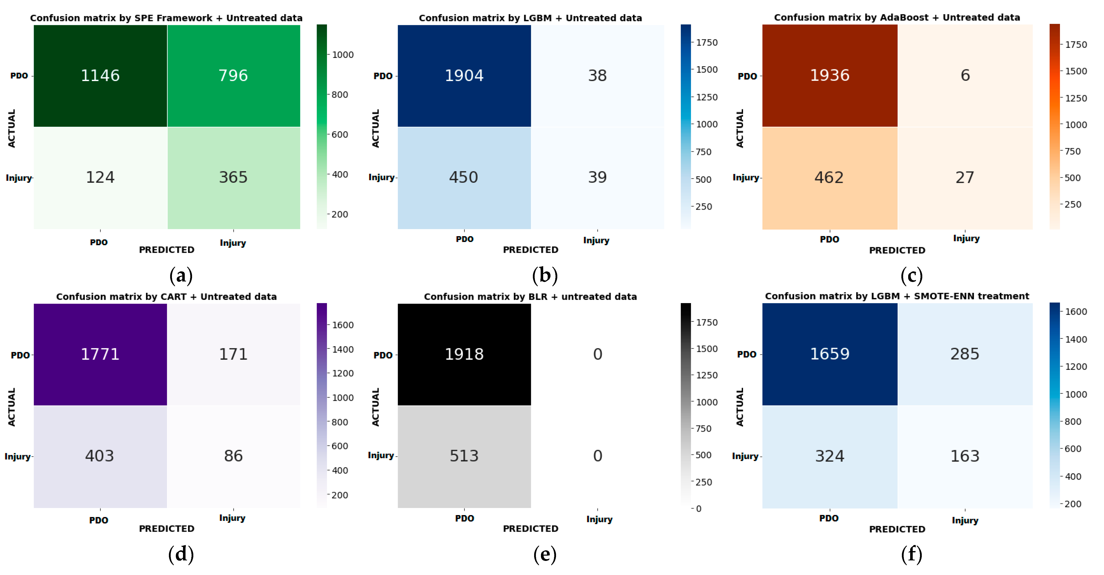
3.3. Model Performance Assessment and Comparison

In this study, the injury and PDO crashes were considered positive and negative classes, respectively, in model development and evaluation. The confusion matrix for the applied models was generated (Figure 9), and the performance measures were quantified as well, including recall value, precision value, G-Mean, and MCC, as shown in

Table 3. Comparison of performance measure of models including SPE, LGBM, AdaBoost, CART, BLR, with no treatment, and SMOTE-ENN treatment.

Models	Treatments	Class	Precision	Recall	G-Mean	MCC
SPE	No Treatment	PDO	0.90	0.56	0.68	0.26
		Injury	0.30	0.78
		Average	0.60	0.67
LGBM		PDO	0.82	0.97	0.55	0.19
		Injury	0.54	0.14
		Average	0.68	0.55
ADABOOST		PDO	0.81	0.91	0.48	0.15
		Injury	0.64	0.06
		Average	0.72	0.48
CART		PDO	0.82	0.89	0.54	0.11
		Injury	0.32	0.20
		Average	0.57	0.55
BLR		PDO	0.79	1.00	0.50	0.01
		Injury	0.00	0.00
		Average	0.39	0.50
LGBM	SMOTE-ENN Treatment	PDO	0.84	0.85	0.59	0.19
		Injury	0.36	0.33
		Average	0.60	0.59
ADABOOST		PDO	0.83	0.84	0.58	0.16
		Injury	0.34	0.31
		Average	0.59	0.58
CART		PDO	0.83	0.85	0.57	0.15
		Injury	0.33	0.29
		Average	0.58	0.57
BLR		PDO	0.80	0.90	0.52	0.08
		Injury	0.28	0.15
		Average	0.54	0.52

.

The recall value showed the models’ ability to correctly classify injury cases, while the precision value revealed the models’ ability to classify PDO cases correctly. It was observed that all models (with and without SMOTE-ENN treatments) were capable of classifying PDO with an accuracy greater than 80%. This was anticipated due to the occurrence of the large number of PDO cases in the work-zone-related crash data set. Regarding recall values, which measure the correct classification of injury crashes, the SPE model using testing data had a 78.16% recall compared to all others, with a recall value between 6.1% and 33.81%. Out of 489 injury crashes, the SPE model classified 365 correctly. It was followed by LGBM with SMOTE-ENN-treated data, which correctly classified 163 out of 489 injuries. The BLR model demonstrated the worst result with no data treatment. None of the injuries were correctly classified out of 489 injuries.

In addition, when compared to all of the other models that included treated and untreated data, the G-Mean for the SPE model was significantly higher. The G-Mean was 0.682 for the SPE model, 0.594 for the LGBM model with SMOTE-ENN-treated data, and 0.581 for the AdaBoost model with SMOTE-ENN treatment. All of these models used the data that were treated with SMOTE-ENN. The G-Mean calculated by the SPE model came out to be around 15.15 percent higher than the G-Mean calculated by the LGBM using SMOTE-ENN-treated data. The SPE model also displayed greater performance in predicting the severity of work zone crash injuries by using the G-Mean as a balanced performance measure between recall and precision values. This was accomplished by using the G-Mean as a performance metric. In our scenario, the MCC value of the SPE model was higher than that of the LGBM, AdaBoost, and CART models, both with and without treatments. This was the case regardless of whether or not the treatments were used. The SPE model showed a higher MCC value compared to other models, with and without data treatment. Based on the performance metrics for all models, the SPE model outperformed the LGBM, AdaBoost, and CART models, indicating the best performance. The SHAP Interpretation system can interpret the results predicted by the SPE model in different ways, such as the relative importance of variables, contributions of variables, and interactions of variables.

3.4. Discussion of Model Result by SHAP

Two methods of interpretation of the SPE model using SHAP are illustrated here, including Global Variable Interpretation and Local Variable Interpretation.

3.4.1. Global Variable Interpretation

There are various ways to determine the relative importance of risk factors. Therefore, risk factor importance and risk factor contribution are not the same. Which factor has the biggest impact on a model’s performance is shown by its contribution. Risk factor contributions identify pertinent elements and offer a logical justification for the observed result (PDO and injuries). This study uses the optimal SPE model to evaluate each risk factor’s significance and contribution to the optimal model’s (SPE) estimation. Figure 10a illustrates the significance of the risk factors, demonstrating the total influence of the risk variables on the forecasts. It is determined by averaging the absolute Shapley values across the entire training dataset. The “Crash Type” variable appears to have the biggest influence on the likelihood of injuries among all the features, as indicated by the mean absolute SHAP value of 0.24. The “Road System” and “Road Median Type” variables are the second and third most significant factors, with average absolute SHAP values of 0.14 and 0.08, respectively. It is least important to consider the “Road Character-Horizontal Alignment” and “Road Surface Type” factors. The remaining factors had only a small impact on the results. A SHAP contribution map of the variables is shown in Figure 10b, which also shows the distribution of SHAP values for each variable and their associated impact patterns. The SHAP value is shown on the horizontal axis of this plot, and the dataset for work zone crashes’ list of variables is shown on the vertical axis. Each point on the plot represents a single SHAP value for a specific prediction and set of variables. Blue color denotes a lower value for a variable, while red color denotes a higher value. One may get an idea of the directionality of the impact of the factors based on the distribution of the red and blue dots. Considering the coding scheme of Table 1 and Figure 10b, the following insights can be drawn from the plot for the top four variables:

• The “Crash Type” variable coded by lower numbers (blue dots), such as 1: Same Direction Rear-End Collision, 2: Side Swipe Same Direction, and 3: Right Angle Collision, has a high positive SHAP value, which increases the likelihood of injuries. Similarly, most of the higher values (red dots), such as collisions with 13: Pedestrian, 14: Pedal Cyclist, and 15: Non-Fixed Object, result in the likelihood of PDO;
• The “Road System” variable coded by lower numbers as well as middle numbers, such as 1: Interstate, 2: State Highway, 3: State/Interstate Authority, 4: State Park or Institution, and 5: County, increases the likelihood of injuries in work zone crashes, whereas most of the higher values, such as 9: Private Property and 10: US Government Property, and few lower numbers increase the likelihood of occurrence of PDO;
• The “Road Medium Type” variable with lower numbers, such as 1: Barrier Median and 2: Curbed Median, increases the likelihood of injuries and vice versa.

3.4.2. Local Variable Interpretation

Figure 11 is a representation of the findings of the model for two cases that were chosen at random as well as the SHAP explanatory force map. If none of the features from the training dataset are used in the current instance, the mean SPE model estimation for the dataset will be 0.5716, which will be the base value. When the output value of the SPE model is lower than the base value, the PDO outcome is the one that is anticipated to occur. When the output value of the SPE Model is greater than the base value, it is anticipated that an injury will occur as a result. The blue arrows represent the degree to which the input variables, also known as risk factors, affect the probability of a particular result. The red arrows in the graph represent the link between the input variables (risk factors) and the probability of an injury becoming the outcome. The amount of influence that each factor has on the final result of the accident is represented by the length (size) of the area that the arrows take up along the horizontal scale. Consider the two scenarios shown in Figure 11 that the SPE model correctly identified as a personal injury and a personal driving offense, respectively.

Figure 11 depicts two instances of correctly classified injuries, and their estimated SPE values are 0.83 and 0.49, respectively. The SPE value for the injury instance is greater than the base value of 0.5716, and the value for the PDO instance is less than the base value. Figure 11a illustrates that the combination of “Crash Type = Rear End Same Direction Collision” and “Light Condition = Dark (Spot Street Lights)”, represented by red arrows pointing to the right, is more likely to result in an injury outcome for the first randomly selected instance. The size of the “Crash Type” arrow is larger than the “Light Condition” arrow, which illustrates that the impact (i.e., explanatory force) of the “Crash Type” variable is greater than that of the “Light Condition” variable in predicting injury for this specific instance. In contrast, for the same case, “Type of Day = Weekend,” illustrated by the blue arrow pointing to the left, illustrates the significance of the risk factor contributing to a PDO outcome in this instance.

Similarly, in Figure 11b, for a case accurately classified as a PDO outcome, the blue arrows “Crash Type = Side Swipe Same Direction Collision”, “Road System = Interstate”, and “Light Condition = Day Light” all point to the left and significantly contribute to a PDO conclusion. However, in the same instance, “Road System = Barrier Median” forces an injury outcome to occur.

3.4.3. Variable Interaction Analysis

The SHAP interaction plots were analyzed in order to comprehend how the input variables used to evaluate the SPE model interact with their contribution to the outcome (see Figure 12). The graph illustrates an interaction study of the four most significant variables: Collision Type, Road System, Road Median Type, and Light Condition. Figure 12a’s scatter plots of red and blue points indicate the variation in Crash Type and Crash Type SHAP values. The SHAP value for Crash Type was larger when Crash Type equals Rear-End Same Direction and Right Angle Collision. Injury was more likely to occur when these types of crashes occur on roads, medians with barriers, and, in rare situations, medians with curbs. The predominance of rear-end same-direction collisions in the injury class shows that relatively high speed mixed with excessively close following was a factor in the injury crashes. These results are in line with the injury severity analysis of Li and Bai from 2006. There might be a possibility that the drivers had limited space in the lane due to lane closure but tried to proceed through the work zone recklessly, attempting an overtaking in congestion. Such conditions increase the likelihood of hitting other vehicles. The occurrence of a higher percentage of injury crashes in the work zone on roads with barrier-type medians was also reported by Koilada et al. [32].

Figure 12b illustrates that the rear-end same-direction and right-angle type crashes are more likely to occur in work zones on New Jersey “state highways”. However, crashes involving animals are more likely to occur on interstate highways. The graph of Light Condition and the SHAP value for Light Condition is depicted in Figure 12c. It shows that the “rear-end same-direction” and “right angle” types of crashes result in injury outcomes during the nighttime with only spot street lights. A likely reason for the higher risk of an injury outcome at night could be associated with the high speeds of vehicles approaching the work zone and poor visibility. Earlier studies on traffic safety reached the same conclusion that rear-end same-direction crashes between vehicles at night increase the risk of injuries [33,34]. Figure 12d shows that the SHAP value for Road System = State Highway is relatively high for the barrier-type median, which means that a large number of injuries occur in this situation. Some of the injuries occur when there is no median. Similarly, almost all of the injury crashes that occur on interstate highways were associated with barrier-type medians. Injury outcomes occur when there is no median or a curbed median.

4. Conclusions and Recommendations

This study utilized a dataset of work zone crashes that transpired on highways within the state of New Jersey during the years 2017 and 2018. The research introduced and contrasted a novel SPE model with tree-based ML and BLR models. The objective was to forecast and classify the severity of work-zone-related crashes while also addressing the issue of imbalance. The utilization of the SHAP interpretative paradigm was employed in tandem with the SPE model to discern primary risk variables and evaluate the magnitude of their influence on the severity of crash outcomes. In this study, the LGBM, AdaBoost, and CART machine learning models were trained using both untreated and treated data to address the issue of data imbalance identified in the preceding section. Nevertheless, the SPE model underwent training and testing using unprocessed data. The SMOTE-ENN technique was employed to enhance the quality of accident data that exhibited significant class imbalance. The results of the experimentation revealed that the SPE model, which relied on raw data of work-zone-related crashes, exhibited superior performance compared to all other tree-based models in the precision, recall, G-Mean, and MCC. The SPE model, which was recently developed, offers a feasible option for assessing the severity of crashes by utilizing crash data that are highly unbalanced. This can be done without the requirement of any pre-processing or treatment of the data.

A frequently expressed concern about machine learning modIls is their deficiIncy in terms of transparency and interpretability. The limited acceptance of models in the engineering domain is impeded due to their greater flexibility and often superior accuracy in comparison to analytical techniques. The interpretability of the SPE model poses a challenge, prompting the utilization of the SHAP approach to elucidate the model outputs. This approach aims to identify the most pertinent risk factors and scrutinize their impact on the severity of work-zone-related crashes. Furthermore, it provides the chance to examine the impacts of risk factors individually and in combination with each other. For instance, it allows for the exploration of whether specific effects may arise in reaction to alterations in the risk variable’s value.

As per the findings, the four primary factors that are highly probable to cause injuries in work zone crashes are “Crash Type”, “Road System”, “Road Median Type”, and “Light Condition”. The impact of “Road Character-Horizontal Alignment” and “Road Surface Type” on the severity of crashes in work zones is minimal. The most injurious collisions are anticipated to be those that occur in the same direction and those that occur at right angles on highways that have barrier-type medians. The study revealed that work zone crashes occurring during nighttime on state highways with localized street lighting were associated with higher injury outcomes.

This study provides an approach that can be utilized to analyze the severity of highway crashes on a broad scale and will be helpful to scholars studying traffic safety and those developing transportation policies. This research examined the SPE model and the SHAP interpretation framework in a case study employing highly unbalanced data of crashes involving work zones. The study is limited to the application of SMOTE-ENN for data balancing. Several other techniques, such as ICOTE (Immune Centroids Oversampling), MTDF (Mega-Trend Diffusion Function), MWMOTE (Majority-Weighted Minority Oversampling Technique), etc. can be taken into account for future research. Similarly, other post hoc interpretation techniques, such as LIME, can also be considered in future studies. Additional research could be conducted by integrating various machine learning methodologies with a range of supplementary risk factors, such as data about the vehicle, time, and driver.

References

1. Federal Highway Administration (FHWA) 2019. Work Zone Facts and Statistics. Available online: https://ops.fhwa.dot.gov/wz/resources/facts_stats.htm#ftn2 (accessed on 17 June 2022).
2. Federal Highway Administration (FHWA) 2017. Facts and Statistics—Work Zone Safety. Available online: http://www.ops.fhwa.dot.gov/wz/resources/factsstats/injuriesfatalities.htm (accessed on 10 July 2017).
3. Theofilatos, A.; Ziakopoulos, A.; Papadimitriou, E.; Yannis, G.; Diamandouros, K. Meta-analysis of the effect of road work zones on crash occurrence. Accid. Anal. Prev. 2017, 108, 1–8. [Google Scholar] [CrossRef] [PubMed]
4. Chen, E.; Tarko, A.P. Modeling safety of highway work zones with random parameters and random effects models. Anal. Methods Accid. Res. 2014, 1, 86–95. [Google Scholar] [CrossRef]
5. Ozturk, O.; Ozbay, K.; Yang, H. Estimating the impact of work zones on highway safety. In Proceedings of the Transportation Research Board 93rd Annual Meeting, Washington, DC, USA, 12–16 January 2014. [Google Scholar]
6. Zha, L.; Lord, D.; Zou, Y. The Poisson inverse Gaussian (PIG) generalized linear regression model for analyzing motor vehicle crash data. J. Transp. Saf. Secur. 2016, 8, 18–35. [Google Scholar] [CrossRef] [Green Version]
7. Li, Z.; Wang, W.; Liu, P.; Bigham, J.M.; Ragland, D.R. Using geographically weighted Poisson regression for county-level crash modeling in California. Saf. Sci. 2013, 58, 89–97. [Google Scholar] [CrossRef]
8. Chen, F.; Chen, S. Injury severities of truck drivers in single-and multi-vehicle accidents on rural highways. Accid. Anal. Prev. 2011, 43, 1677–1688. [Google Scholar] [CrossRef]
9. Ye, F.; Lord, D. Investigation of effects of under reporting crash data on three commonly used traffic crash severity models: Multinomial logit, ordered probit, and mixed logit. Transp. Res. Rec. 2011, 2241, 51–58. [Google Scholar] [CrossRef]
10. Marzoug, R.; Lakouari, N.; Ez-Zahraouy, H.; Téllez, B.C.; Téllez, M.C.; Villalobos, L.C. Modeling and simulation of car accidents at a signalized intersection using cellular automata. Phys. A Stat. Mech. Its Appl. 2022, 589, 126599. [Google Scholar] [CrossRef]
11. Weng, J.; Meng, Q.; Wang, D.Z. Tree-based logistic regression approach for work zone casualty risk assessment. Risk Anal. 2013, 33, 493–504. [Google Scholar] [CrossRef]
12. Morgan, J.F.; Duley, A.R.; Hancock, P.A. Driver responses to differing urban work zone configurations. Accid. Anal. Prev. 2010, 42, 978–985. [Google Scholar] [CrossRef]
13. Weng, J.; Xue, S.; Yang, Y.; Yan, X.; Qu, X. In-depth analysis of drivers’ merging behavior and rear-end crash risks in work zone merging areas. Accid. Anal. Prev. 2015, 77, 51–61. [Google Scholar] [CrossRef]
14. Bai, Y.; Yang, Y.; Li, Y. Determining the effective location of a portable changeable message sign on reducing the risk of truck-related crashes in work zones. Accid. Anal. Prev. 2015, 83, 197–202. [Google Scholar] [CrossRef] [PubMed]
15. McAvoy, D.S.; Duffy, S.; Whiting, H.S. Simulator study of primary and precipitating factors in work zone crashes. Transp. Res. Rec. 2011, 2258, 32–39. [Google Scholar] [CrossRef]
16. Weng, J.; Du, G.; Ma, L. Driver injury severity analysis for two work zone types. In Proceedings of the Institution of Civil Engineers-Transport; Thomas Telford Ltd.: London, UK, 2016; Volume 169, pp. 97–106. [Google Scholar]
17. Li, Y.; Bai, Y. Highway work zone risk factors and their impact on crash severity. J. Transp. Eng. 2009, 135, 694–701. [Google Scholar] [CrossRef]
18. Osman, M.; Paleti, R.; Mishra, S.; Golias, M.M. Analysis of injury severity of large truck crashes in work zones. Accid. Anal. Prev. 2016, 97, 261–273. [Google Scholar] [CrossRef]
19. Akhter, M.N.; Mekhilef, S.; Mokhlis, H.; Mohamed Shah, N. Review on forecasting of photovoltaic power generation based on machine learning and metaheuristic techniques. IET Renew. Power Gener. 2019, 13, 1009–1023. [Google Scholar] [CrossRef] [Green Version]
20. Zhang, J.; Li, Z.; Pu, Z.; Xu, C. Comparing prediction performance for crash injury severity among various machine learning and statistical methods. IEEE Access 2018, 6, 60079–60087. [Google Scholar] [CrossRef]
21. Sarkar, S.; Pramanik, A.; Maiti, J.; Reniers, G. Predicting and analyzing injury severity: A machine learning-based approach using class-imbalanced proactive and reactive data. Saf. Sci. 2020, 125, 104616. [Google Scholar] [CrossRef]
22. Beam, A.L.; Kohane, I.S. Big data and machine learning in health care. Jama 2018, 319, 1317–1318. [Google Scholar] [CrossRef]
23. Dixon, M.F.; Halperin, I.; Bilokon, P. Machine Learning in Finance; Springer International Publishing: Berlin/Heidelberg, Germany, 2020. [Google Scholar]
24. Lundberg, S.M.; Lee, S.I. A unified approach to interpreting model predictions. Adv. Neural Inf. Process. Syst. 2017, 30. [Google Scholar]
25. Dong, S.; Khattak, A.; Ullah, I.; Zhou, J.; Hussain, A. Predicting and analyzing road traffic injury severity using boosting-based ensemble learning models with SHAPley Additive exPlanations. Int. J. Environ. Res. Public Health 2022, 19, 2925. [Google Scholar] [CrossRef]
26. Yang, C.; Chen, M.; Yuan, Q. The application of XGBoost and SHAP to examining the factors in freight truck-related crashes: An exploratory analysis. Accid. Anal. Prev. 2021, 158, 106153. [Google Scholar] [CrossRef] [PubMed]
27. Chawla, N.V.; Lazarevic, A.; Hall, L.O.; Bowyer, K.W. SMOTEBoost: Improving prediction of the minority class in boosting. In Proceedings of the InKnowledge Discovery in Databases: PKDD 2003: 7th European Conference on Principles and Practice of Knowledge Discovery in Databases, Cavtat-Dubrovnik, Croatia, 22–26 September 2003; Springer: Berlin/Heidelberg, Germany, 2003; pp. 107–119. [Google Scholar]
28. Liu, Z.; Cao, W.; Gao, Z.; Bian, J.; Chen, H.; Chang, Y.; Liu, T.Y. Self-paced ensemble for highly imbalanced massive data classification. In Proceedings of the 2020 IEEE 36th International Conference on Data Engineering (ICDE), Dallas, TX, USA, 20 April 2020; IEEE: Piscataway, NJ, USA, 2020; pp. 841–852. [Google Scholar]
29. Wu, J.; Chen, X.Y.; Zhang, H.; Xiong, L.D.; Lei, H.; Deng, S.H. Hyperparameter optimization for machine learning models based on Bayesian optimization. J. Electron. Sci. Technol. 2019, 17, 26–40. [Google Scholar]
30. Dimitrijevic, B.; Khales, S.D.; Asadi, R.; Lee, J.; Kim, K. Segment-Level Crash Risk Analysis for New Jersey Highways Using Advanced Data Modeling; Center for Advanced Infrastructure and Transportation, Rutgers University: New Brunswick, NJ, USA, 2020. [Google Scholar]
31. Dimitrijevic, B.; Khales, S.D.; Asadi, R.; Lee, J. Short-term segment-level crash risk prediction using advanced data modeling with proactive and reactive crash data. Appl. Sci. 2022, 12, 856. [Google Scholar] [CrossRef]
32. Koilada, K.; Mane, A.S.; Pulugurtha, S.S. Odds of work zone crash occurrence and getting involved in advance warning, transition, and activity areas by injury severity. IATSS Res. 2020, 44, 75–83. [Google Scholar] [CrossRef]
33. Lee, C.; Li, X. Analysis of injury severity of drivers involved in single-and two-vehicle crashes on highways in Ontario. Accid. Anal. Prev. 2014, 71, 286–295. [Google Scholar] [CrossRef]
34. Dimitrijevic, B.; Asadi, R.; Spasovic, L. Application of hybrid support vector Machine models in analysis of work zone crash injury severity. Transp. Res. Interdiscip. Perspect. 2023, 19, 100801. [Google Scholar] [CrossRef]
Figure 1. Model for the prediction and analysis of work-zone related crash injury severity.
Sustainability 15 09076 g001
Figure 2. Risk variables in work-zone-related crashes with their relative frequencies, (a) Road character-Horizontal alignment, (b) Road character- Grade, (c) Road surface type, (d) Road surface condition, (e) Light condition, (f) Environmental condition, (g) Road median type, (h) Temporary traffic control zone, (i) Road system, (j) Crash type, (k) Type od Day, (l) Number of vehicle involved.
Sustainability 15 09076 g002aSustainability 15 09076 g002bSustainability 15 09076 g002c
Figure 3. Injury severity distribution in original work zone crash data.
Sustainability 15 09076 g003
Figure 4. Procedure of SMOTE-ENN algorithm.
Sustainability 15 09076 g004
Figure 5. Classification and regression tree (CART) as A: Decisiom node, B and C: Terminal Node.
Sustainability 15 09076 g005
Figure 6. Tree expansion in LGBM.
Sustainability 15 09076 g006
Figure 7. Confusion matrix plot.
Sustainability 15 09076 g007
Figure 8. Injury severity distribution in (a) Untreated training data, (b) SMOTE_ENN treatment.
Sustainability 15 09076 g008
Figure 9. Confusion matrices of the (a) SPE Framework with untreated data, (b) LGBM with untreated data, (c) AdaBoost with untreated data, (d) CART with untreated data, (e) BLR with untreated data, (f) LGBM with SMOTE-ENN treatment, (g) AdaBoost with SMOTE-ENN treatment, (h) CART with SMOTE-ENN treatment, (i) BLR with SMOTE-ENN treatment.
Sustainability 15 09076 g009aSustainability 15 09076 g009b
Figure 10. Global Variable Interpretation: (a) variable importance plot; (b) variable contribution plot.
Sustainability 15 09076 g010
Figure 11. SHAP force plot: (a) for an instance value equals 0.83; (b) for an instance value equals 0.49.
Sustainability 15 09076 g011
Figure 12. SHAP interaction plots: (a) interaction of Crash Type and Road Median Type; (b) interaction of Road System and Crash Type; (c) interaction of Light Condition and Crash Type; (d) interaction of Road System and Road Median Type.
Sustainability 15 09076 g012aSustainability 15 09076 g012b