An Approach for the Classification of Rock Types Using Machine Learning of Core and Log Data

Abstract

Classifying rocks based on core data is the most common method used by geologists. However, due to factors such as drilling costs, it is impossible to obtain core samples from all wells, which poses challenges for the accurate identification of rocks. In this study, the authors demonstrated the application of an explainable machine-learning workflow using core and log data to identify rock types. The rock type is determined utilizing the flow zone index (FZI) method using core data first, and then based on the collection, collation, and cleaning of well log data, four supervised learning techniques were used to correlate well log data with rock types, and learning and prediction models were constructed. The optimal machine learning algorithm for the classification of rocks is selected based on a 10-fold cross-test and a comparison of AUC (area under curve) values. The accuracy rate of the results indicates that the proposed method can greatly improve the accuracy of the classification of rocks. SHapley Additive exPlanations (SHAP) was used to rank the importance of the various well logs used as input variables for the prediction of rock types and provides both local and global sensitivities, enabling the interpretation of prediction models and solving the “black box” problem with associated machine learning algorithms. The results of this study demonstrated that the proposed method can reliably predict rock types based on well log data and can solve hard problems in geological research. Furthermore, the method can provide consistent well log interpretation arising from the lack of core data while providing a powerful tool for well trajectory optimization. Finally, the system can aid with the selection of intervals to be completed and/or perforated.

1. Introduction

The classification of rocks is a research topic of common interest among geologists. The accurate classification of rocks can help geologists and petrophysicists determine the sedimentary environments to improve the accuracy of well log interpretation. With the rapid development of electronics and information technology in recent years, researchers have started using machine learning techniques to investigate the relationship between well log data, rock types, and established methods for predicting rock types. Machine learning uses various algorithms to build a predictive model on the basis of available data. The advantage of this method is that it can evaluate the effect of multiple parameters on output simultaneously, which is difficult to study manually. Therefore, machine learning is especially effective for high-dimensional problems such as rock type classification. These techniques can be classified into supervised and unsupervised learning techniques. Supervised learning techniques use machine learning for model training and prediction based on rock types identified by geologists. Hall [1] established a lithology identification method based on support vector machines. Nishitsuji et al. [2] believed that deep learning has greater potential in lithology identification. Yang Xiao et al. [3] used a decision tree learning algorithm to classify volcanic rocks. Valentín et al. [4] identified rock types using a deep residual network based on acoustic image logs and micro-resistivity image logs. Unsupervised learning techniques use training samples of unknown categories (unlabeled training samples) to solve various problems in pattern recognition. Commonly used unsupervised learning algorithms include principal component analysis (PCA) and clustering algorithms. Ding Ning [5] carried out lithology identification by means of cluster analysis based on density attributes. Ju Wu et al. [6] identified coarse-grained sandstone, fine-grained sandstone, and mudstone using a Bayes stepwise discriminant analysis method with an accuracy of 82%. Duan Youxiang et al. [7] improved the accuracy of sandstone identification and classification to a level higher than that of methods based on single-machine learning. Ma Longfei et al. [8] built a model based on a gradient-boosted decision tree (GBDT) that can improve the accuracy of lithology identification. Most of these methods use mathematical models for lithology identification based on manually determined rock types and involve great uncertainties because experts may adopt different criteria for the classification of rocks. Moreover, these methods mainly focus on sandstone reservoirs; they only use a certain type of algorithm for lithology identification and do not consider the optimization of models adequately. Therefore, it is difficult to interpret the final models of these methods with geological knowledge. Tang et al. [9] used machine learning to find the optimum profile in shale formations. Zhao et al. [10] used machine learning methods to study the dynamic characteristics of fractures in different shale fabric facies, which showed that machine learning can solve more complex problems, such as shale rock fabric and fracture characteristics. In this paper, a method combining FZI and machine learning is proposed for the first time to realize the classification of rock types in the study area. The rock type is determined through the FZI method using core data, then by comparing the accuracy levels of four machine learning algorithms and selecting the optimal algorithm to identify rock types in uncored wells. This method can be used to identify rocks in various hydrocarbon reservoirs and improve the efficiency and accuracy of well log interpretation and other geological interpretations. It provides a new idea for lithology identification and is of great significance for intelligent reservoir evaluation.

2. Geological Settings

The study area is located in the northeastern part of the Amu Darya basin in Turkmenistan, near the juncture with Uzbekistan. The formation of interest is composed of the Callovian–Oxfordian carbonate deposits, with an estimated thickness of 350 m, consisting of the following units from top to bottom: XVac, XVp, XVm, XVhp, XVa1, Z, XVa2, and XVI [11] (Figure 1).

The area under study in the Callovian period is a carbonate gentle slope sedimentary system composed of an inner ramp, a mid-ramp, an outer ramp, and basin facies belts. In the early Oxfordian period, under regional transgression, the outer zone of the mid ramp and outer ramp in the Callovian period were gradually submerged, and the inner ramp—mid-ramp gradually developed into an edged shelf-type carbonate platform. The water body in the outer zone is highly energetic, and high-energy shoals or reef–shoal complexes were developed. The top of the reservoir starts at a depth of about 2300 m. The main production zones are XVac, XVp, and XVm. The main rock types are various limestones, where the average matrix porosity is 11.1% and the geometric mean of permeability is 53 mD. The reservoir space can be summarized into three types: pore, vug, and fracture. The reservoir quality varies significantly vertically and laterally due to different depositional settings and diagenesis.

3. Data and Methodology

The schematic of the workflow used in this work is shown in Figure 2.

3.1. Data

In this study, the 270 m coring data of 3 wells in the Callovian–Oxfordian formation were used, mainly including the routine core analysis data of 956 samples, core photos, thin sections, and scanning electron microscope data of 3 wells. In addition, petrophysical well-log data, including gamma-ray (GR), sonic (DT), resistivity (RT and RXO), and density (RHOB) logs, were available for rock-type classification, especially in the intervals with poor core data or without core data.

3.2. Methods

3.2.1. Rock Types

Rock typing has a wide variety of applications, such as the prediction of high mud-loss intervals, potential production zones, and locating perforations. There are many methods to classify rock types; in this study, we use Winland r₃₅ [12], Pittman equations [13], and the FZI [14] method. A detailed method of rock classification can be found in the related literature. It can be seen from Figure 3 that the Callovian–Oxfordian formation in the study area can be divided into 7 rock types (DRT 1–DRT 7). The corresponding rock types are wackstone with microporosity, mud-dominated packstone, grainstone with some separate-vug pore space, grainstone, grain-dominated packstone, wackstone with microfractures, and mudstone with microfractures, respectively. The microscopic photos of different rock types are shown in Figure 4. Statistics of the porosity and permeability of different rock types are shown in

Table 1. Porosity, permeability, and lithology by rock type.

Rock Types	Median Porosity (%)	Median Permeability (mD)	Lithology
DRT1	4.18	0.002	Wackstone with microporosity
DRT2	8.60	0.300	Mud-dominated packstone
DRT3	11.90	5.100	Grainstone with some separate-vug pore space
DRT4	12.00	30.300	Grainstone
DRT5	1.68	1.750	Grain-dominated packstone
DRT6	1.00	1.840	Wackstone with microfracture
DRT7	0.38	0.490	Mudstone with microfracture

.

3.2.2. Data Preprocessing

The data preprocessing consists of three main phases: data collection, data cleaning and feature selection, correlation, and normalization.

(1) Data collection

Having the right data is essential in research work to ensure its success. The authors collected different rock types (DRTS) and corresponding logging data from 3 wells. The log data included laterolog deep (RT), laterolog shallow (RXO), acoustic log (DT), which reflects sedimentation and diagenesis, and gamma log (GR), which reflects sedimentation. The statistical characteristics of the collected data are shown in

Table 2. Statistical distribution of the log data set.

	DT	GR	RHOB	RT	RXO
	(us/ft)	(gAPI)	(g/cm3)	(ohm·m)	(ohm·m)
Number of values	1093.00	1093.00	1093.00	1093.00	1093.00
Number of missing	2.00	2.00	2.00	2.00	2.00
Min value	48.86	5.29	1.57	4.51	3.53
Max value	81.70	42.94	2.67	72,207.00	618.60
Mode	55.08	8.76	2.41	26.86	10.24
Arithmetic mean	61.83	16.25	2.38	372.28	56.98
Geometric mean	61.41	14.74	2.38	52.46	22.87
Median	60.87	15.01	2.39	33.46	15.92
Average deviation	6.17	5.87	0.07	566.01	65.06
Standard deviation	7.35	7.04	0.10	3307.82	103.48
Variance	54.05	49.58	0.01	10,941,600.00	10,707.70
Skewness	0.39	0.59	−1.82	17.44	2.91
Kurtosis	−0.73	−0.30	8.88	325.68	8.34
Q1 [10%]	52.79	7.64	2.27	15.81	7.31
Q2 [25%]	55.55	10.58	2.33	22.55	9.68
Q3 [50%]	60.87	15.01	2.39	33.46	15.92
Q4 [75%]	67.03	21.50	2.44	79.79	37.78
Q5 [90%]	72.31	26.29	2.48	488.06	176.45

, with the structured document containing 1093 rows and 6 columns representing rock types and features, respectively.

It can be seen from

Table 3. Average values of logging parameters for different rock types.

Rock Types	GR	RHOB	DT	RT	RXO
	(gAPI)	(g/cm3)	(us/ft)	(ohm·m)	(ohm·m)
DRT1	16.70	2.41	54.50	50.70	41.00
DRT2	17.00	2.41	59.50	30.30	17.90
DRT3	11.30	2.39	62.70	38.60	17.10
DRT4	13.00	2.34	63.80	90.90	30.10
DRT5	16.30	2.32	59.30	262.10	91.10
DRT6	16.80	2.29	54.50	650.00	208.90
DRT7	17.20	2.31	57.60	786.00	311.50

that the GR value of different types of rocks is low and changes little, and the RHOB value also does not change much. The DT value of DRT 3 and DRT 4 is larger (greater than 60 gAPI) than that of other rock types, reflecting the characteristics of high porosity, while DRT 6 and DRT 7 have high resistivity (RT and RXO) values, which reflect the compact characteristics of these two rocks.

It can be seen from the star-plot of average logging values of different rock types (Figure 5) that it is difficult to use one or several logging values to classify rock types, which further illustrates the necessity of building other models (such as machine learning) to predict rock types.

(2) Data cleaning and feature selection

Data cleaning is the process of detecting and removing noisy data (erroneous, inconsistent, and duplicate data) from datasets. Erroneous data mainly results from errors in well log data (especially density data) and is typically caused by borehole enlargement during the drilling process. In this study, erroneous data is mainly identified through statistical analysis methods (e.g., box-plot method). Duplicate data mainly originates from different rock types or porosity and permeability values at the same depth. In addition, some columns in the initial dataset are empty, and the authors analyzed the “missingness” in the data set, which represents the percentage of the total number of entries for any variable that is missing. The missing values can either be predicted using the other variables or removed. The missingness of well-logging variables used in this study is shown in Figure 6, in which the X-axis represents the well-logging variable and the Y-axis represents the missingness expressed as a percentage. Since, the degree of missingness is very low (<0.4%) in this data set, the rows with missing values were removed.

Outliers were removed mainly through the histogram method, the box-plot method, and Rosner’s test [15]. Histograms are useful to provide information on the distribution of values for each feature; they can be used to determine the distribution, center, and skewness of a dataset and detect outliers therein. From the frequency histograms of various parameters (Figure 7), it can be seen that RT and RXO data follow a skewed distribution, and ROHB data basically follow a normal distribution. A few outliers are shown as black circles in the figure.

Box plots are widely used to describe the distribution of values along an axis based on the five-number summary: minimum, first quartile, median, third quartile, and maximum (Figure 8). This visual method allows the reviewer to better understand the distribution and locate the outliers. The median marks the midpoint of the data and is shown by the line that divides the narrow box into two. The median of the data is usually skewed towards the top or bottom of the narrow box, which means that the data are usually denser on the narrow side. Two of the more extreme examples are RT and RXO. In the samples that the authors took, half of the samples had values between 30 and 50 ohm·m, which is a relatively dense range. The box plot represents a left-skewed distribution. The values that are greater than the upper limit or lesser than the lower limit will be the outliers that should be further looked into as they might carry extra information. Most features do not have outliers, and only the RHOB values of some sample points are less than 2.0 g/m³. These values are outliers resulting from the distortion of density data caused by borehole collapse during the drilling process.

Considering the fact that this study involves a large number of samples, the authors used the Rosner test function to detect the outliers [16]. The function performs the Rosner generalized extreme studentized deviate test to identify potential outliers in a data set, assuming the data without any outliers comes from a normal (Gaussian) distribution.

(3) Correlation

By understanding the correlation between different parameters, appropriate features can be selected to build models. Ideally, features that provide a clear relationship to the output while avoiding too many similar features that would present duplicate information should be selected. In order to determine if parameters are linearly correlated with each other, the Pearson correlation coefficient was used to calculate the correlation between various parameters; the calculation formula is as follows [17]:

$$r=\frac{1}{n-1}(\frac{{\sum }_x{\sum }_y(x-\overline{x})(y-\overline{y})}{S_x{S}_y})$$

(1)

where $n$ is the number of paired data; $\stackrel{-}{x}$ and $\stackrel{-}{y}$ are the sample means; and $S_x$ and $S_y$ are the sample standard deviations of all the $x$ values and all the $y$ values, respectively. The coefficient value can range between −1.00 and 1.00. A negative value indicates the relationship between the variables is negatively correlated, which means as one value increases, the other decreases. Vice versa, a positive value tells us that the relationship between the variables is positively correlated, which means that as one value increases, the other also increases. As shown in Figure 9, the parameters are poorly correlated, and only the RXO and DT parameters have a strong negative correlation (r is −0.45).

(4) Normalization

To meet the needs of some machine learning algorithms (such as KNN), the data needs to be normalized to eliminate bias. There are several techniques to scale or normalize the data. The standard scaler expressed by Equation (2) was used for this study. For any given set of data, $x_i$

$$x_{scaled\_i}=\frac{x_i-mean\left(x\right)}{StdDev\left(x\right)}$$

(2)

3.2.3. Machine Learning

Machine learning is a process that allows a computer to learn from data without being explicitly programmed, where an algorithm (often a black box) is used to infer the underlying input/output relationship from the data [18]. There are various machine learning algorithms, but they are generally categorized into supervised and unsupervised learning. Supervised algorithms learn from labeled data, while unsupervised methods automatically mine or explore for patterns based on similarities. The optimal algorithm among four supervised learning classifiers (KNN, MLP, RF, and GBM) was selected through a comparative performance analysis and used to predict rock types.

(1) Random Forest (RF)

The random forest method is an ensemble learning method based on decision tree learning [19]. The goal of decision tree learning is to create a model that predicts the value of a target variable based on several input variables by discretizing the multidimensional sample space into uniform blocks and using the average value within each block as the predictive value. The disadvantage of decision tree learning is that, for complex problems, the tree tends to grow excessively, resulting in overfitting. The random forest method solves the problem of overfitting by creating a large number of deep decision trees [20]. In each tree, a random subset of the input attributes (log variables) is used to split the tree at any node. This randomization across multiple trees (random forest) avoids the overfitting problem associated with single decision trees by averaging the prediction results of all trees. Furthermore, the relative importance of each input feature can be ranked in the random forest model. Larger importance means that a decision on the basis of that specific input can result in greater homogeneity in the subtrees. Typically, nodes at the top of the decision tree have higher importance. Figure 10 shows that RT is the most important of the five logging parameters for rock classification.

The random forest method can obtain the optimal result and avoid overfitting by adjusting the maximum tree depth, the percentage of features used in each tree, and the minimum sample size in a leaf node. Figure 11a shows the optimal number of parameters for splitting at any node, which should be 11.

(2) Gradient Boosting Machine (GBM)

Both GBM and the random forest method belong to the broad class of tree-based classification techniques. A series of weak learners is initially generated, each of which fits the negative gradient of the loss function of the previously superimposed model, so that the cumulative loss of the model after the addition of the weak learner decreases in the direction of the negative gradient. Then, all learners are linearly combined using different weights to enable the learners with excellent performance to be reused. The major advantage of the GBM algorithm is that it does not require standardization or normalization of features when different types of data are used; it is not sensitive to missing data; and it features high nonlinearity and good interpretability for the model.

Optimizable hyperparameters in the GBM algorithm include the number of trees, the minimum number of data points in the leaf nodes, the interaction depth specified for the maximum depth of each tree, and the number of variables (or predictors) for splitting at each node [21]. The larger the number of trees, the larger the tree depth, and the higher the accuracy. The smaller the number of observations at leaf nodes, the higher the accuracy. When there are more than 800 trees and the maximum tree depth is 15, the complexity of the model will increase greatly, but the improvement in accuracy is negligible. Therefore, simpler models are preferred to avoid overfitting. The optimal hyperparameters selected for this study are as follows: the number of trees (estimators) is 172 (Figure 11b), the maximum tree depth is 3, the minimum number of samples for a leaf node is 1, the number of features to be split is 0.2, and the number of random states (random seeds) is 89.

(3) K-Nearest Neighbor (KNN)

KNN is a nonparametric regression and classification technique that uses a predefined number of nearest neighbors to determine the new value (for regression) or new label (for classification) of new observations [22,23]. It usually uses the Euclidean distance to measure the distance between two points or elements. To prevent the weights of attributes with larger initial values (such as RT and RXO in this study) from exceeding those of attributes with smaller initial values (such as RHOB in this study), each value needs to be normalized or standardized before the weights of attributes are calculated.

The tuning hyperparameter for the KNN technique is the number of the nearest neighbors K that can be evaluated by a trial-and-error approach. It can be seen from Figure 11c that, when K is greater than 40, the accuracy of the model will decrease as the number of neighbors increases. Therefore, the optimal number of neighbors is 40.

(4) Multilayer-Perceptron Neural Network (MLP)

Multilayer-perceptron neural networks are fully connected feed-forward networks, which are best applied to problems where the input data and output data are well defined, yet the process that relates the input to the output is extremely complex [24,25]. A neural network usually consists of multiple layers; each layer has several neurons, and the neurons in one layer are connected to all neurons in adjacent layers. Each neuron receives one or more input signals (such as well-logging variables considered herein), and the input signals are multiplied by corresponding weights to generate output signals (such as rock types). The relationship between the independent variable $x$ and the dependent variable $y$ can be expressed as:

$$y\left(x\right)=f({\sum }_{i=1}^n{w}_i{x}_i)$$

(3)

The $w$ weights allow each of the $n$ inputs (denoted by $x_i$) to contribute a greater or lesser amount to the sum of input signals. For the activation function $f\left(x\right)$, the net sum is used, and the resulting signal $y\left(x\right)$ is the output.

The main adjustable parameters in the MLP algorithm are the number of layers and the number of neurons (or nodes) in each layer. Errors can be minimized by optimizing the weights. The optimal parameters are as follows: Alpha is 0.0001, bet_1 is 0.9, and bet_2 is 0.999. An MLP is optimal when it consists of three hidden layers and the number of neurons in the third hidden layer is 14 (Figure 11d).

Figure 11. Hyperparameter tuning for different supervised learning (a) the Estimators of RF is 11. (b) the Estimators of GBM is 172. (c) the K of KNN is 40. (d) the number of neurons in the third hidden layer is 14.

Figure 11. Hyperparameter tuning for different supervised learning (a) the Estimators of RF is 11. (b) the Estimators of GBM is 172. (c) the K of KNN is 40. (d) the number of neurons in the third hidden layer is 14.

3.3. K-Fold Cross-Validation

Classifiers for lithology identification were constructed using KNN, GBM, random forest, and MLP based on well log data. The log parameters selected for predicting the rock types were GR, RT, DT, RXO, and RHOB. A total of 75% of the data was used for training, and the other 25% was used for testing. A 10-fold cross-validation was performed on the training data to prevent overfitting. In 10-fold cross-validation, the training data were randomly subdivided into 10 parts; the model was trained on 9 parts and then validated on the remaining 1 part. This process was repeated multiple times for each machine learning technique. Only those models were averaged to give the final model that provides good results on the validation data. Figure 11 shows the results for hyperparameter tuning, and

Table 4. Summary of optimal hyperparameters for different supervised learnings.

Methods	Optimal Hyperparameter Values
KNN	Number of neighbors = 40
MLP neural network	Layer1: units = 15; Layer2: units = 20; Layer3: units = 14
Random forest	N-Estimators = 11
GBM	N-Estimators = 172, maximum tree depth = 3, n.minobsinnode = 1 (minimum number of observations in the leaf nodes = 1)

summarizes the optimal values of hyperparameters for different supervised learning techniques.

Table 5. Summary of cross-validation accuracy for different supervised learnings.

Machine Learning Algorithms	Cross Validation Accuracy (%)	Cross Validation Standard Deviation (%)
GBM	67.86	3.22
MLP	67.01	2.37
KNN	67.03	0.10
Random forest	66.88	2.69

summarizes the cross-validation accuracy for different supervised learnings.

4. Evaluation and Application of Machine Learning

4.1. Model Accuracy and Machine Learning Results

Table 6. Different accuracy metrics on the test data set for different supervised learnings.

Machine Learning Algorithms	AUC	Model Accuracy (%)
GBM	0.83	79.25
MLP	0.78	73.94
KNN	0.75	70.85
Random forest	0.74	70.40

summarizes the different accuracy metrics on the test data set for different supervised learning techniques. The area under the curve (AUC) represents the area under the receiver operating characteristic (ROC) curve and is a useful metric to evaluate the performance of any classification model [26]. The accuracy metric represents the proportion of the test data set predicted correctly (expressed as a percentage). It can be seen from Table 6 that the four supervised learning techniques have achieved prediction results, and their accuracy levels are higher than 70%. The GBM has achieved the highest accuracy and largest AUC value, indicating that it is the best one among the four supervised learning techniques in terms of performance. The model accuracy has reached 79.25% on the test set.

Figure 12 shows the results of a comparison between the actual rock types (Actual Rock types) of core samples from Well A (which was not modeled during this study) and the rock types predicted by various supervised learning techniques (different colors represent different rock types). GBM_Rock represents rock types predicted by GBM using the log data. MLP_Rock, KNN_Rock, and Rand Forest_Rock represent the results predicted using MLP, KNN, and random forest, respectively. It is evident that the random forest technique does not predict as well as other supervised learning techniques. The visual results in Figure 12 further corroborate the quantitative accuracy metrics shown in Table 6.

4.2. Importance of Predictors and Model Interpretation

Prediction models can be interpreted by quantitatively analyzing the importance of predictors (well-logging variables) to the models. This is helpful in decoding the “black box” predictions and makes the model interpretable. The main parameter is the SHapley Additive exPlanations (SHAP) values, which are calculated for each combination of predictor (log variables) and cluster (rock types). Mathematically, they represent the average of the marginal contributions across all permutations [27]. Typically, a higher SHAP value for a predictor/cluster combination suggests that the chosen log variable is important to identify the cluster. Because SHAP is model-agnostic, any machine-learning model can be analyzed to derive input/output relationships.

Figure 13a shows a variable-importance plot that lists the most significant variables in descending order, which provides a global interpretation of the classification and shows the average impact on model-output magnitude. In Figure 13a, the X-axis represents the average value of the SHAP absolute value, which reflects the average effect on the magnitude of the output, and the Y-axis represents the well-logging variables used to identify rock types. The plot shows that RT, RXO, and DT are the three most important variables to define rock types in this study.

Figure 13b shows the SHAP values for Cluster 3 (Rock type 4) and different log variables; the different points represent the different observations (i.e., depths in the data set). The color in the plot represents whether the log variable has a high or low value for that observation. The X-axis shows the Shapley values; the larger the Shapley value, the greater the impact on cluster prediction. For any variable, such as RHOB, the SHAP values corresponding to different RHOB data points range from slightly negative to larger positive values. The points with larger positive SHAP values have a strong influence on Rock type 4, and these points are associated with low (colored blue) values of features, suggesting that low RHOB values are a key characteristic of Rock type 4. Similarly, it can be determined through analysis that low GR values and high DT values are also typical features of Rock type 4. In summary, Cluster 3 (rock type 4) is characterized by low GR values, low RHOB values, high DT values, and medium-high RXO values, which is consistent with the rocks in Cluster 3 being grainstones with low GR values, low RHOB values, high DT values, and low RT values. This method is helpful in the local interpretation of classification models. Such analysis provides a way to interpret classification results without considering model selection, and the application of SHAP values in petroleum engineering provides a method for the global and local interpretation of classification models.

5. Conclusions

This paper presents a promising and interpretable machine learning approach that can identify various types of rocks based on well log data. The purpose of this study was to improve geological insights and the accuracy of well log interpretation through accurate identification of rock types. The proposed method also provides valuable references for the optimization of well trajectory and the optimal selection of intervals to be perforated. The conclusions drawn from this study are detailed below.

(1)

Based on core data and the FZI method, the Callovian–Oxfordian formation in the study area can be divided into seven rock types.

(2)

The results of this study show that the rock types in uncored wells can be accurately classified by core data using machine learning and well log data. Accurate classification of rocks can greatly improve the accuracy of well log interpretation and the reliability of research results with respect to sedimentary microfacies.

(3)

Four machine learning algorithms were evaluated, including KNN, GBM, random forest, and MLP. Based on the cross-validation and evaluation results, the GBM has been selected for the identification of rock types in the study area. The accuracy of this algorithm for lithology identification can reach 79%.

(4)

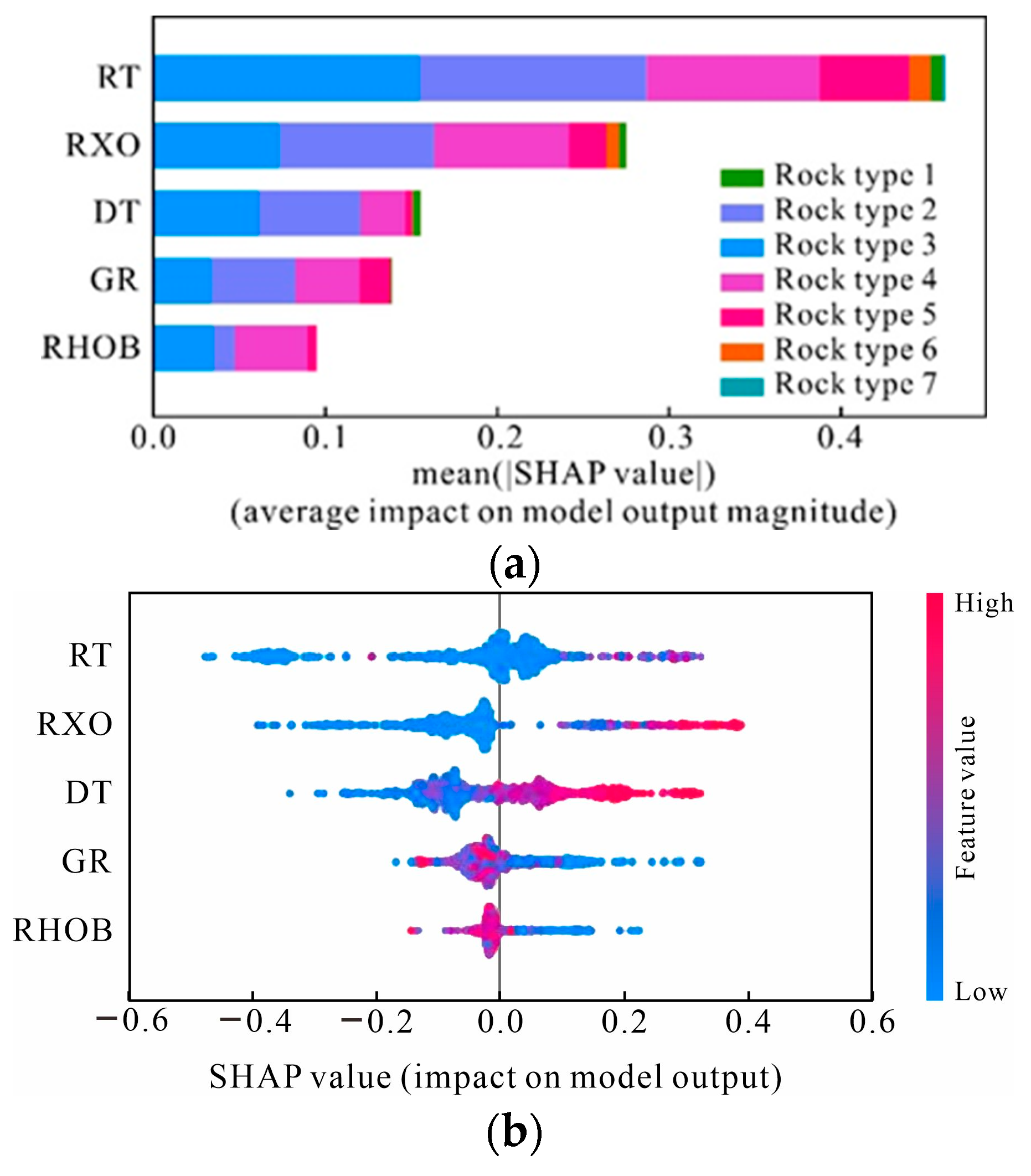
In this study, SHAP values were used to interpret “black box” (machine learning) models, which demonstrate high robustness and practicability and provide an effective means of global and local interpretation for rock classification models based on machine learning.

(5)

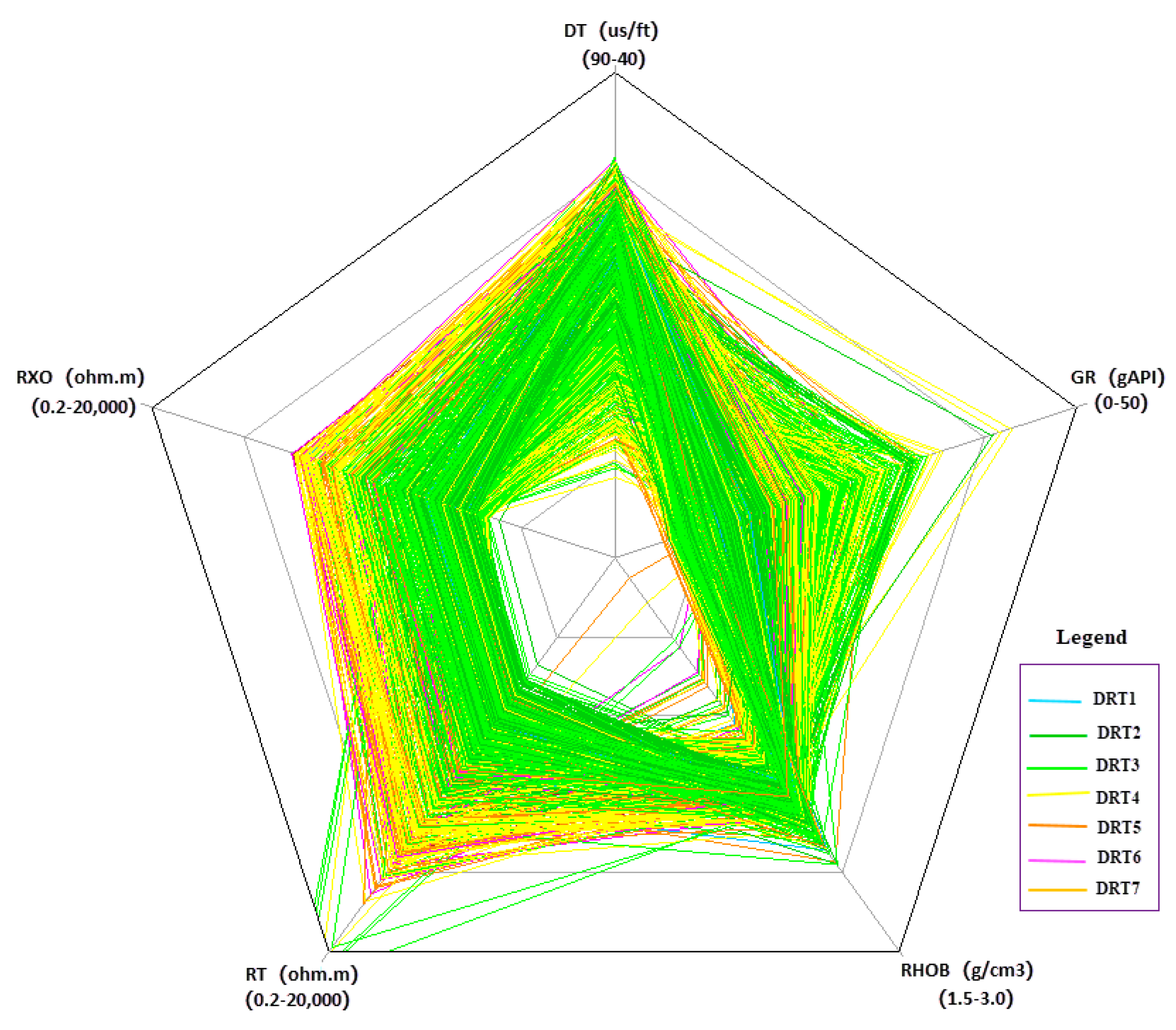
The results of this study suggested that Rock type 4 (grainstones) are the best reservoir rocks in the study area. These rocks are characterized by high porosity, high permeability, low GR values, low RHOB values, high DT values, low RT values, and low RXO values.

References

1. Brendon Hall. Facies classification using machine learning. Lead. Edge 2016, 35, 906–909. [Google Scholar] [CrossRef]
2. Nishitsuji, Y.; Exley, R. Elastic impedance-based facies classification using support vector machine and deep learning. Geophys. Prospect. 2019, 67, 1040–1054. [Google Scholar] [CrossRef]
3. Xiao, Y.; Wang, Z.; Zhou, Z.; Wei, Z.; Qu, K.; Wang, X.; Wang, R. Lithology classification of acidic volcanic rocks based on parameter-optimized Ada Boost algorithm. Acta Pet. Sin. 2019, 40, 457–467. [Google Scholar]
4. Valentin, M.B.; Bom, C.R.; Coelho, J.M.; Correia, M.D.; De Albuquerque, M.P.; de Albuquerque, M.P.; Faria, E.L. A deep residual convolutional neural network for automatic lithological facies identification in Brazilian pre-salt oilfield wellbore image logs. J. Pet. Sci. Eng. 2019, 179, 474–503. [Google Scholar] [CrossRef]
5. Ning, D. An Improved Semi Supervised Clustering of Given Density and Its Application in Lithology Identification; China University of Geosciences: Beijing, China, 2018. [Google Scholar]
6. Ju, W.; Han, X.H.; Zhi, L.F. A lithology identification method in Es4 reservoir of xin 176 block with bayes stepwise discriminant method. Comput. Tech. Geophys. Geochem. Explor. 2012, 34, 576–581. [Google Scholar]
7. Duan, Y.; Wang, Y.; Sun, Q. Application of selective ensemble learning model in lithology-porosity prediction. Sci. Technol. Eng. 2020, 20, 1001–1008. [Google Scholar]
8. Ma, L.; Xiao, H.; Tao, J.; Su, Z. Intelligent lithology classification method based on GBDT algorithm. Pet. Geol. Recovery Effic. 2022, 29, 21–29. [Google Scholar]
9. Tang, J.; Fan, B.; Xiao, L.; Tian, S.; Zhang, F.; Zhang, L.; Weitz, D. A New Ensemble Machine Learning Framework for Searching Sweet Spots in Shale Reservoirs. SPE J. 2021, 26, 482–497. [Google Scholar] [CrossRef]
10. Zhao, X.; Jin, F.; Liu, X.; Zhang, Z.; Cong, Z.; Li, Z.; Tang, J. Numerical study of fracture dynamics in different shale fabric facies by integrating machine learning and 3-D lattice method: A case from Cangdong Sag, Bohai Bay basin, China. J. Pet. Sci. Eng. 2022, 218, 110861. [Google Scholar] [CrossRef]
11. Ulmishek, G.F. Petroleum Geology and Resources of the Amu Darya Basin, Turkmenistan, Uzbekistan, Afghanistan and Iran; USGS: Reston, VA, USA, 2004; pp. 1–38. [Google Scholar]
12. Kolodzie, S. Analysis of pore throat size and use of the Waxman-Smits equation to determine OOIP in Spindle field, Colorado. In Proceedings of the SPE Annual Technical Conference and Exhibition, Dallas, TX, USA, 21–24 September 1980. SPE-9382-MS. [Google Scholar]
13. Pittman, E.D. Relationship of porosity and permeability to various parameters derived from mercury injection-capillary pressure curves for sandstone. AAPG Bull. 1992, 76, 191–198. [Google Scholar]
14. Amaefule, J.O.; Altunbay, M.; Tiab, D.; Kersey, D.G.; Keelan, D.K. Enhanced reservoir description using core and log data to identify hydraulic flow units and predict permeability in un-cored intervals/wells. In Proceedings of the SPE Annual Technical Conference and Exhibition, Houston, TX, USA, 3–6 October 1993. [Google Scholar]
15. Tang, Q. DPS Data Processing System—Experimental Design, Statistical Analysis and Data Mining, 2nd ed.; Science Press: Beijing, China, 2010. [Google Scholar]
16. Barnett, V.; Lewis, T. Outliers in Statistical Data, 3rd ed.; John Wiley & Sons: Chichester, UK, 1995. [Google Scholar]
17. Hu, L.; Gao, W.; Zhao, K.; Zhang, P.; Wang, F. Feature Selection Considering Two Types of Feature Relevancy and Feature Interdependency. Expert Syst. Appl. 2018, 93, 423–434. [Google Scholar] [CrossRef]
18. Breiman, L. Arcing the Edge; Technical Report 486; Statistics Department, University of California, Berkeley: Berkeley, CA, USA, 1997. [Google Scholar]
19. Breiman, L. Random Forests. Mach. Learn. 2001, 45, 5–32. [Google Scholar] [CrossRef]
20. Kuhn, S.; Cracknell, M.J.; Reading, A.M. Lithological mapping in the Central African copper belt using random forests and clustering: Strategies for optimised results. Ore Geol. Rev. 2019, 112, 103015. [Google Scholar] [CrossRef]
21. Kuhn, M. Building Predictive Models in R Using the caret Package. J. Stat. Softw. 2008, 28, 1–26. [Google Scholar] [CrossRef]
22. Altman, N.S. An Introduction to Kernel and Nearest-Neighbor Nonparametric Regression. Am. Stat. 1992, 46, 175–185. [Google Scholar]
23. James, G.; Witten, D.; Hastie, T.; Tibshirani, R. An Introduction to Statistical Learning with Applications in R; Springer: New York, NY, USA, 2013. [Google Scholar]
24. LeCun, Y.; Bottou, L.; Bengio, Y.; Haffner, P. Gradient-Based Learning Applied to Document Recognition. Proc. IEEE 1998, 86, 2278–2324. [Google Scholar] [CrossRef]
25. Nielson, M.A. Neural Networks and Deep Learning; Determination Press: San Francisco, CA, USA, 2015. [Google Scholar]
26. Fawcett, T. An Introduction to ROC Analysis. Pattern Recognit. Lett. 2006, 27, 861–874. [Google Scholar] [CrossRef]
27. Lundberg, S.M.; Lee, S.I. A Unified Approach to Interpreting Model Predictions. In Proceedings of the 31st Conference on Neural Information Processing Systems, Long Beach, CA, USA, 4–9 December 2017. [Google Scholar]
Figure 1. Location of the study area and the column for target intervals of Callovian–Oxfordian.
Sustainability 15 08868 g001
Figure 2. Schematic of the workflow presented in this work.
Sustainability 15 08868 g002
Figure 3. Porosity and permeability cross-plots of different rock types identified by FZI.
Sustainability 15 08868 g003
Figure 4. Photomicrographs of 7 rock types identified in the Callovian–Oxfordian stage.
Sustainability 15 08868 g004
Figure 5. Star-plots of log mean values for different rock types.
Sustainability 15 08868 g005
Figure 6. Missingness in different variables used in this study.
Sustainability 15 08868 g006
Figure 7. Histograms of features (log parameters).
Sustainability 15 08868 g007
Figure 8. Box plot of features (log parameters).
Sustainability 15 08868 g008
Figure 9. Correlation of features (log parameters).
Sustainability 15 08868 g009
Figure 10. The plot of feature importance.
Sustainability 15 08868 g010
Figure 12. The plot of actual rock types and the types predicted by different machine learning techniques.
Sustainability 15 08868 g012
Figure 13. (a) Variable importance plot. (b) Sharp plot for Rock type 4.
Sustainability 15 08868 g013