Adaptability Evaluation of the Spatiotemporal Fusion Model of Sentinel-2 and MODIS Data in a Typical Area of the Three-River Headwater Region

Abstract

The study of surface vegetation monitoring in the “Three-River Headwaters” Region (TRHR) relies on satellite data with high spatial and temporal resolutions. The spatial and temporal fusion method for multiple data sources can effectively overcome the limitations of weather, the satellite return period, and funding on research data to obtain data higher spatial and temporal resolutions. This paper explores the spatial and temporal adaptive reflectance fusion model (STARFM), the enhanced spatial and temporal adaptive reflectance fusion model (ESTARFM), and the flexible spatiotemporal data fusion (FSDAF) method applied to Sentinel-2 and MODIS data in a typical area of the TRHR. In this study, the control variable method was used to analyze the parameter sensitivity of the models and explore the adaptation parameters of the Sentinel-2 and MODIS data in the study area. Since the spatiotemporal fusion model was directly used in the product data of the vegetation index, this study used NDVI fusion as an example and set up a comparison experiment (experiment I first performed the band spatiotemporal fusion and then calculated the vegetation index; experiment II calculated the vegetation index first and then performed the spatiotemporal fusion) to explore the feasibility and applicability of the two methods for the vegetation index fusion. The results showed the following. (1) The three spatiotemporal fusion models generated high spatial resolution and high temporal resolution data based on the fusion of Sentinel-2 and MODIS data, the STARFM and FSDAF model had a higher fusion accuracy, and the R2 values after fusion were higher than 0.8, showing greater applicability. (2) The fusion accuracy of each model was affected by the model parameters. The errors between the STARFM, ESTARFM, and FSDAF fusion results and the validation data all showed a decreasing trend with an increase in the size of the sliding window or the number of similar pixels, which stabilized after the sliding window became larger than 50 and the similar pixels became larger than 80. (3) The comparative experimental results showed that the spatiotemporal fusion model can be directly fused based on the vegetation index products, and higher quality vegetation index data can be obtained by calculating the vegetation index first and then performing the spatiotemporal fusion. The high spatial and temporal resolution data obtained using a suitable spatial and temporal fusion model are important for the identification and monitoring of surface cover types in the TRHR.

1. Introduction

At present, remote sensing technology is an important tool for conducting large-scale vegetation cover distribution research. In addition, long-term time series of remote sensing image data can provide a data base for monitoring changes in vegetation cover, extracting weather information, identifying grass species and crops, etc. [1]. For example, surface weather information can be extracted by constructing NDVI and LSWI time series to inform ground crop management [2]. There are also many studies that monitor surface plant virus infections or species invasion using remote sensing time series data [3]. However, it is difficult for a single type of remote sensing images to meet the application requirements of high temporal resolution and high spatial resolution. Meanwhile, data quality problems will inevitably occur due to weather factors such as rain and snow [4,5]. The spatiotemporal fusion model can effectively alleviate the mutual constraints of the temporal and spatial resolutions, and effectively solve the problem of cloud or shadow contamination in the time series of satellite image data to improve the image quality.

After years of development, spatiotemporal fusion models have become relatively mature, and existing spatiotemporal data fusion methods can be categorized into three groups: weighted function based, unmixing based, and dictionary pair learning based [6]. Some scholars have optimized combinations of these types models to improve their applicability. Among them, Gao et al. proposed the spatial and temporal adaptive reflectance fusion model (STARFM) [7] to fuse Landsat and MODIS surface reflectance data, and achieved good results. However, its fusion in complex surface landscape areas was poor. Zhu et al. proposed the enhanced spatial and temporal adaptive reflectance fusion model (ESTARFM) [8] based on the STARFM, which improved the accuracy of predicting fine-resolution reflectance data, especially for heterogeneous landscapes with better preservation of their spatial details. In order to better capture the reflectance changes caused by land cover conversion, Zhu et al. proposed the flexible spatiotemporal data fusion model (FSDAF) [6], which required less modeling data and could effectively capture heterogeneous landscapes. For different spatiotemporal data fusion models, several scholars have conducted comparative studies from various perspectives, such as the data applicability and regional applicability of the models. Among them, Wu et al. combined Landsat-ETM+ and MODIS data to compare and analyze the specific application capabilities of five models, including the STARFM and ESTARFM under complex conditions in southern China [9]. Using the STIFM [10], STDFM [11], and ESTARFM, Shi Yuezen et al. compared and analyzed their effectiveness in fusing MODIS and ASTER/TM data in the Yingke irrigation area [12], and their results showed that the STDFM was better for fusion in the red band and the ESTARFM was suitable for fusion in the near-red band. Hobyb et al. applied three models, i.e., the STARFM, ESTARFM and FSDAF, to fuse Landsat 8 and MODIS data to generate high spatial and temporal resolution NDVI data [13], and their results showed that the ESTARFM algorithm worked optimally and could effectively deal with the propagation of errors. Hu et al. performed the image fusion of Landsat 9 OLI and MODIS NDVI data using the STARFM, ESTARFM, FSDAF, and GF-SG models [5], and their experiments demonstrated that the GF-SG could generate higher accuracy NDVI data in grassland, forest, and farmland test areas. However, the results suffered from the over-smoothing phenomenon, which was more serious in high-heterogeneity areas. On the data scale of the spatiotemporal fusion model, most of the data with low and medium spatial resolutions, such as MODIS, AVHRR, and TM, were used for fusion studies [14]. With the development of remote sensing technology, satellite images with higher spatial resolution are being put into use, and the data selection for the fusion models becomes a necessary issue to explore. Additionally, in general, the smaller the width of satellite images with a high spatial resolution, the smaller the width of the images, and the complexity for data processing will be increased. Applying the traditional spatiotemporal fusion model to two data sources with large-scale differences will need to be studied for its adaptability.

Previous studies have shown that the spatiotemporal fusion model is closely related to the data used for fusion, ground cover, and other factors. As an important ecological protection area in China, the monitoring of vegetation coverage and changes in the TRHR has received much attention [15,16]. High-quality land surface phenology data as long-term time series are helpful in identifying and monitoring the vegetation composition, especially toxic weeds, in the TRHR [17]. Sentinel-2 image data can provide high-quality image data with a temporal resolution of 5 days and a spatial resolution of 10 m due to the complementary nature of its two satellites [18], which provides a good data choice for continuous monitoring of vegetation cover changes in the TRHR. However, due to the complex climate changes in the TRHR, there are more clouds and rainy weather, and the quality of Sentinel-2 image data is seriously affected by weather. Meanwhile, the MODIS image has a re-entry period of less than 1 day, and the data are more selective, which makes them more conducive to the construction of time series data. However, due to the lower spatial resolution of MODIS data, they are not suitable for high-accuracy vegetation cover and grass species identification. Therefore, the complementary MODIS and Sentinel-2 data are expected to generate high-quality spatial and temporal resolution data, which can effectively improve the accuracy of grass species identification and the temporal accuracy of grass cover changes in the TRHR. Meanwhile, most studies have focused on assessing the fusion of MODIS and Landsat imagery data [19,20,21], but there is a lack of studies on the fusion of Sentinel-2 and MODIS data to generate higher resolution fusion data in the TRHR. In addition, when the existing studies applied the spatiotemporal fusion model to the surface vegetation cover, the fusion was generally performed directly using the vegetation index to save research time. However, some studies have shown that the timing of the spatiotemporal fusion impacted the accuracy of the NDVI, and this view needs to be further explored in this study area. Therefore, in this paper, three fusion models, the STARFM, ESTARFM, and FSDAF, were used to evaluate the suitability of fusing Sentinel-2 and MODIS data in the TRHR [22]. Since the methodological principles of the fusion models differ, their parameter settings also vary. Parameter sensitivity experiments were conducted simultaneously during the adaptation assessment, so that the more suitable fusion models within the optimal parameter values could be compared. Using the parameters with the best fusion effects, the influence of the NDVI spatiotemporal fusion timing on the accuracy was investigated in two ways: (1) the spatiotemporal fusion of the red and near-red bands was performed first followed by the NDVI generation, and (2) the NDVI calculation was performed first followed by the fusion. Finally, the most suitable spatiotemporal fusion method was obtained for a typical area of Sanjiangyuan, and high spatiotemporal resolution data with a spatial resolution of 10 m and temporal resolution of 1 day were generated to visualize the grass dead cover and grass changes in the TRHR.

2. Materials and Methods

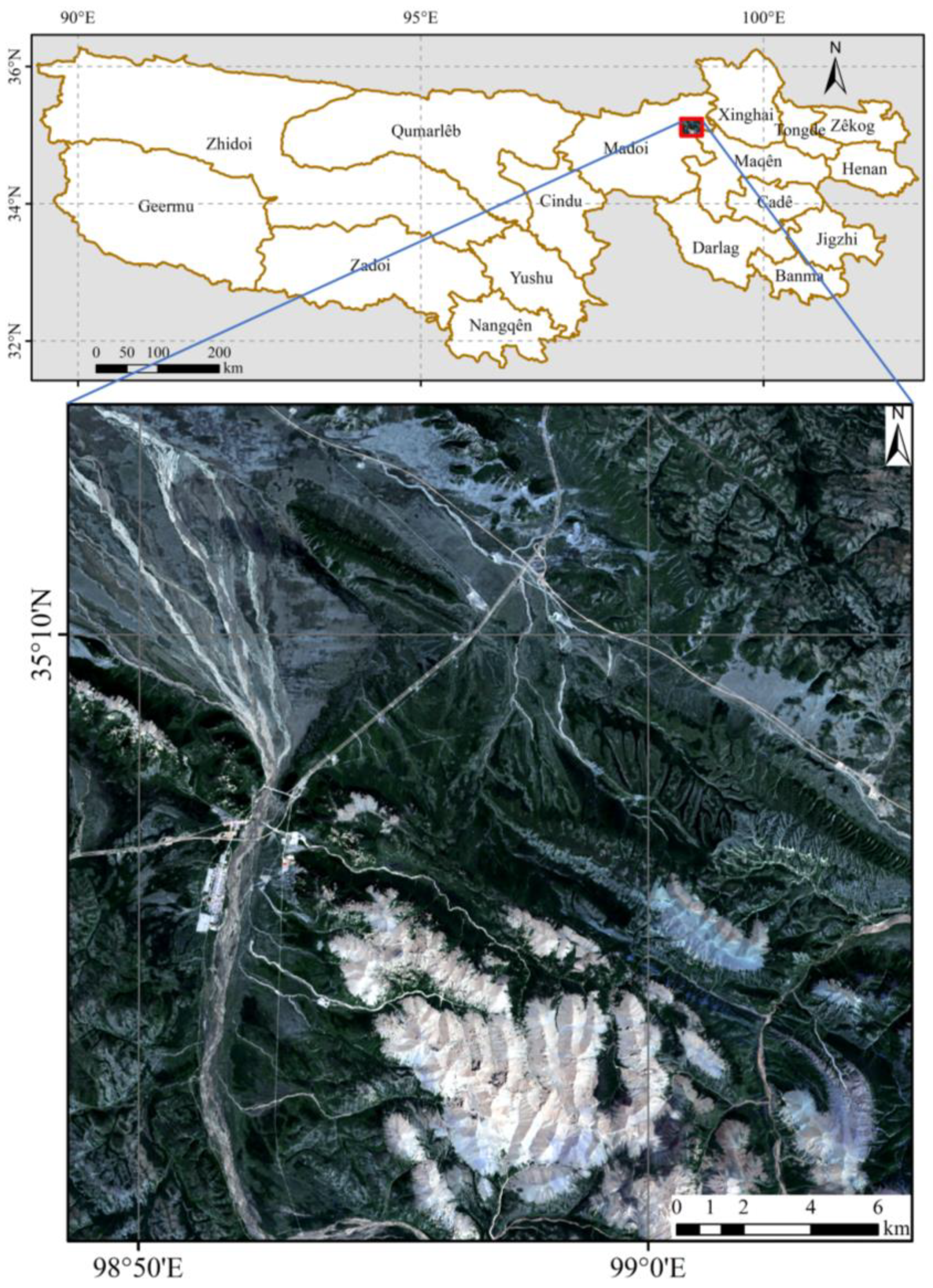
2.1. Study Area

The study area of this paper was located in Huashixia Town, northeast of Maduo County, Qinghai Province. The study area covered 38°43′10″ to 38°59′57″ north latitude and 48°06′25″ to 50°56′56″ east longitude, and the average elevation was 4500 m. The climate was characterized by long, cold, dry, and windy winters and short, cool, and rainy summers. The annual average temperature of Maduo County was −4.1 °C, with a large daily difference in the temperature, no absolute frost-free period throughout the year, and an annual average precipitation of 303.9 mm with large inter-year variations. The meadow area of Maduo County accounts for 87.5% of the total land area of the county, and the available meadow area is 1,805,300 hectares, accounting for 78.5% of the meadow area. The meadow type is mainly alpine meadow. The area has the highest concentration of biodiversity in high-altitude regions in the world, and the uniqueness and vulnerability of the vegetation are well documented [23].

The lack of rational use and protection, coupled with the impact of rodent infestation, has led to a gradual decline in the dominant populations of the meadows in this region. The invasion of a large number of grass species that are not preferred by animals, toxic subdominant species, or companion species in the community has led to the serious degradation of the alpine meadows [24,25]. The basis for the management of meadow degradation is the timely and accurate identification of its ecological community structure changes, and the use of satellite remote sensing images with a wide detection range and efficient data collection for identification. Due to the special local geographical environment, a single remote sensing data source can hardly meet the monitoring requirements for the meadow population structure changes, and there is an urgent need to construct remote sensing time series data with high spatial and temporal resolutions for monitoring these regions. This is the significance of this study. To carry out the relevant research, we selected a specific area in the TRHR, as shown in Figure 1.

2.2. Data

In this paper, the data from the Sentinel-2 Level-1C and MODIS surface reflectance daily product MOD09GQ1 covering the study area were selected as the experimental data. The Sentinel-2 data were downloaded from the ESA Copernicus Open Access Hub (https://scihub.copernicus.eu/dhus, accessed on 26 January 2022) and the MODIS data were downloaded from the NASA data website (https://ladsweb.modaps.eosdis.nasa.gov, accessed on 11 March 2022). The Band4 and Band8 bands of the Sentinel-2 images corresponded to the Band1 and Band2 bands of the MODIS images, respectively, belonging to the red and near-infrared bands. The two bands of the Sentinel-2 data had a spatial resolution of 10 m, with two complementary satellites and a re-entry period of 5 days. The two bands of the MODIS data had a spatial resolution of 250 m and a temporal resolution of 1 day. The specific band correspondence information is shown in

Table 1. The data band information for the Sentinel-2 and MODIS data sets.

Data Set	Band	Spatial Resolution/(m)	Temporal Resolution/(day)
Sentinel-2 Level-1C	Band4 (R)	10	5
	Band8 (NIR)	10	5
MODIS MOD09GQ1	Band1 (R)	250	1
	Band2 (NIR)	250	1

.

The MODIS images for 25 April, 25 July, and 30 July 2019, and the Sentinel-2 images for 26 April, 25 July, and 30 July 2019 (the Sentinel-2 data in this study area had high cloudiness on the day of 25 April, and it was generally believed that the surface changes during the three days were extremely subtle) were selected as three periods of cloud-free data for the experiment in this study, all containing both red and near-red bands.

The L1C-level data of Sentinel-2 were orthoimagery with geometrically refined correction and no atmospheric correction. The images were first atmospherically corrected using the Sen2cor plug-in to generate the L2A-level data, and then cropped to obtain the study area data and calculate the NDVI using Equation (1).

$$NDVI=\frac{B_{NIR}-B_R}{B_{NIR}+B_R}$$

(1)

where $B_{NIR}$ and $B_R$ represent the near-red and red bands of the image, respectively. The MODIS surface reflectance data products were atmospherically corrected and needed to be projectionally converted to WGS_1984_UTM and resampled to 10 m to be consistent with the Sentinel-2 data, followed by cropping of the study area and calculating the NDVI.

2.3. Methods

The overall technical methodology of this paper is shown in Figure 2, which consists of three parts.

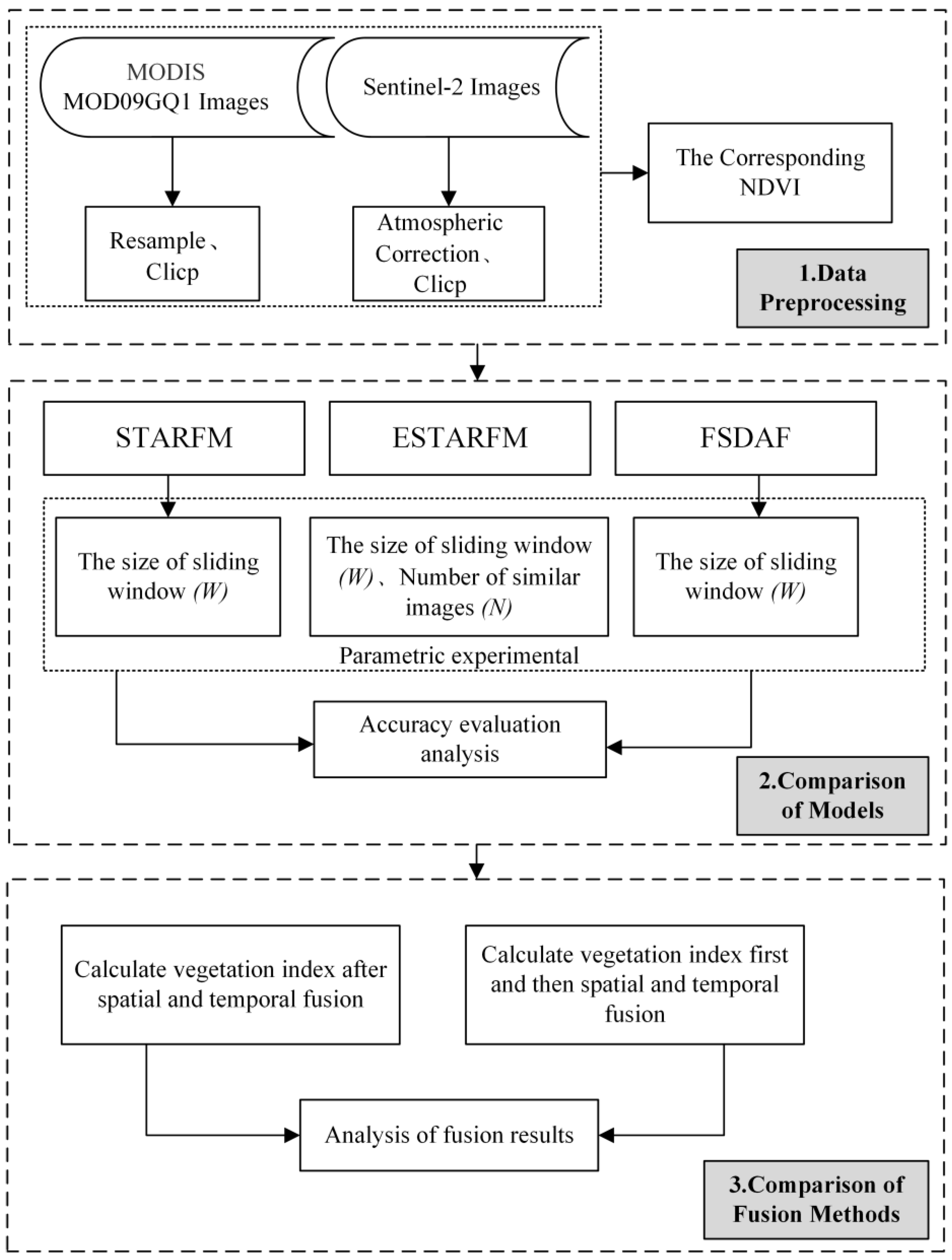
(i)

Data pre-processing. The pre-processing of the acquired raw Sentinel-2 and MODIS data to obtain the red and near-red band data and NDVI data with a uniform resolution and projection coordinates in the study area.

(ii)

Experimental analysis of the fusion models. The parameters of the STARFM, ESTARFM, and FSDAF model were set using the control variable method, and the fused red band, near-red band, and NDVI data were obtained under various combinations of parameters. The accuracy indexes of the fused data of each model were compared separately, and their applicability and optimal parameter range in the typical area of the TRHR were analyzed.

(iii)

Comparative analysis of the fusion schemes. Based on the best parameters for the fusion model experiments, a comparative experimental scheme was designed based on the NDVI (in experiment Ⅰ the band fusion was performed first and then the vegetation index was calculated; in experiment Ⅱ the vegetation index was calculated first and then the spatiotemporal fusion was performed) to compare the fusion results of experiments Ⅰ and Ⅱ and to discuss the feasibility of conducting spatiotemporal fusion experiments based directly on the vegetation index data products.

2.3.1. Fusion Method

1.

STARFM

The STARFM algorithm was proposed by Gao et al. and used to fuse Landsat and MODIS images [7]. The algorithm was developed based on a linear mixture model, which assumes that the image element values of high spatial resolution images do not change even if the image element values of low spatial resolution do not change, and that the image element values corresponding to equal values at the initial moment are still equal at the same moment thereafter. In the case of neglecting the error, the relationship between the reflectance of the image elements with different spatial resolutions is shown in Equation (2).

$$L(x_i,y_i,t_k)=M(x_i,y_i,t_k)+{\epsilon }_k$$

(2)

where $L(x_i,y_i,t_k)$ and $M(x_i,y_i,t_k)$ are the reflectance values of the high spatial resolution and high temporal resolution images at the t_k moment $(x_i,y_i)$, respectively, and ${\epsilon }_k$ is their reflectance difference. Under the assumptions that the systematic errors of t₀ and t_k and the type of ground cover are constant, ${\epsilon }_0={\epsilon }_k$. Therefore, this can be written as Equation (3).

$$L(x_i,y_i,t_k)=M(x_i,y_i,t_k)+L(x_i,y_i,t_0)-M(x_i,y_i,t_0)$$

(3)

Since the hypothetical conditions are influenced by mixed image elements and land cover changes in reality, the neighboring image pixel weight matrix (Equation (4)) can be introduced.

$$L(x_{\omega /2},y_{\omega /2},t_k)={\displaystyle {\sum }_{i=1}^{\omega }{\displaystyle {\sum }_{j=1}^{\omega }{\displaystyle {\sum }_{k=1}^n{W}_{ijk}\times \left. [M(x_i,y_i,t_k)+L(x_i,y_i,t_0)-M(x_i,y_i,t_0)\right]}}}$$

(4)

where $\omega$ is the size of the moving window, $(x_{\omega /2},y_{\omega /2})$ are the center image element position, and $W_{ijk}$ is the weight matrix. The main parameters in the application of the model are the size of the moving window and the type of ground cover.

2.

ESTARFM

The ESTARFM algorithm was proposed by Zhu et al. to improve the spatiotemporal fusion accuracy in the more heterogeneous regions based on the STARFM by considering the trend of reflectivity over time [8]. If any element within the moving window satisfies Equation (5) with the central image element, it is identified as the central image element.

$$\left|L(x_i,y_i,t_k)-L(x_{\frac{\omega }{2}},y_{\frac{\omega }{2}},t_k)\right|\le 2\sigma /m$$

(5)

where $\sigma$ is the standard deviation of the image element reflectance within the moving window and $m$ is the number of feature types. The central image element reflectance of the predicted image is calculated by introducing similar image elements of the adjacent spectrum within the sliding window, as shown in Equation (6).

$$L(x_{\omega /2},y_{\omega /2},t_k)=L(x_{\omega /2},y_{\omega /2},t_0)+{\displaystyle {\sum }_{i=1}^N{W}_i{V}_i\times \left. [M(x_i,y_i,t_k)-M(x_i,y_i,t_0)\right]}$$

(6)

where N is the number of similar pixels and $W_i$ and $V_i$ are the weight factor and conversion factor of the i-th similar pixel to the central image, respectively. The ESTARFM algorithm is mainly influenced by the type of ground cover, sliding window size, and the number of similar images.

3.

FSDAF

FSDAF is a flexible spatiotemporal data fusion method proposed by Zhu [6], which first performs an unsupervised classification of the high spatial resolution image at a time point, then estimates the change in the category corresponding to the low spatial resolution image at another time point, predicts the high spatial resolution image at the second time point based on this change, and assign the residuals (Equation (7)).

$$\Delta P(x_i,y_i)=P_0(x_i,y_i)-P_k(x_i,y_i)$$

(7)

where $\Delta P$ denotes the difference between the pixels at the moments $t_0$ and $t_k$. In practice, the corresponding image elements of the two time points are considered to have different effects on the classification, and the residuals need to be assigned to them. The model introduces the TPS function to improve the accuracy of the residual assignment, and the predicted image value can be derived from Equation (8) after calculating the residuals and weights.

$$\Delta P(x_{ij},y_{ij})={\displaystyle \sum _{j=1}^n{K}_j}\times \Delta P(x_i,y_i)+R(x_{ij},y_{ij})$$

(8)

where $K_j$ is the weight of the class j and R is the residual. The main parameters of the FSDAF algorithm are the type of ground cover and the sliding window size.

2.3.2. Fusion Model Parameter Sensitivity Experiments

In this paper, we compared three widely used remote sensing spatiotemporal fusion models: the STARFM, ESTARFM, and FSDAF. Combining the model principles and existing studies [6,7,8,22,26], the fusion accuracy effect of the STARFM and FSDAF model was mainly influenced by the size of the sliding window and the number of feature types in the study area. The ESTARFM introduced the neighboring homogeneous image elements with similar spectral characteristics as the auxiliary information to improve the fusion accuracy. Therefore, the effect of the sliding window size and the number of feature types on the fusion accuracy of the model should not only be considered, but the effect of the change in the number of similar image elements on the fusion effect of the model should also be explored.

The STARFM and FSDAF model in the study required a high spatial resolution image, a low spatial resolution image, and a high temporal resolution image as the input data for modeling, while the ESTARFM required two corresponding high- and low-resolution images as the input data for modeling. The red band, near-red band data, and NDVI index data from Sentinel-2 and MODIS on 25 July 2019 were selected to train the STARFM and FSDAF model. For the ESTARFM, the MODIS data from 25 April and 25 July 2019 were selected as the low-resolution training data and the Sentinel-2 data from 26 April and 25 July 2019 were selected as the high resolution training data for modeling. All three models were used to predict the fusion of the MODIS data from 30 July 2019 to generate the corresponding high-resolution data, and the real Sentinel-2 image data from 30 July 2019 were used for the comparative analysis and accuracy evaluation. The information on the experimental data corresponding to the specific models is shown in

Table 2. Description of the experimental data.

Method	Input Data						Validation Data
	Sentinel-2			MODIS			Sentinel-2
	Band	Resolution	Date	Band	Resolution	Date	Band	Resolution	Date
STRAFM	R/NIR	10 m	25 July 2019	R/NIR	250 m	25 July 2019	R/NIR	10 m	30 July 2019
			-			30 July 2019
ESTARFM	R/NIR	10 m	26 April 2019	R/NIR	250 m	25 April 2019	R/NIR	10 m	30 July 2019
			25 July 2019			25 July 2019
			-			30 July 2019
FSDAF	R/NIR	10 m	25 July 2019	R/NIR	250 m	25 July 2019	R/NIR	10 m	30 July 2019
			-			30 July 2019

.

In this study, the optimal ranges of the model-related parameters were explored separately using control variables. According to the preliminary field survey and remote sensing image interpretation, the surface cover types in this study area were relatively simple and could be roughly divided into four categories: vegetation, bare soil, snow/clouds, and others. Therefore, the number of surface cover types for all three models in this experiment was set to four. For the STARFM, the surface cover category was set to four, the sliding window size was W ($\mathrm{W}=\omega /2$), the W step size was five pixels, and the experimental fusion prediction was in the range of W = 5~70 pixels for the case of the 30 July high-resolution data. For the ESTARFM, the sensitivity of the sliding window size W was investigated by keeping the number of similar pixels N constant, and the value of W was the same as above. When the sensitivity of the number of similar pixels N was investigated, the size of the sliding window W was controlled to be constant, with a step size W of 5, and the fusion used the high-resolution data from 30 July with N ranging from 15 to 130. For the FSDAF model, Zhu et al. showed that the accuracy of the fusion results was stable when the number of similar image elements N > 20 [6]. To save computational time, N was set to 25 in this study and the sliding window size W was set as above.

The applicability of the spatiotemporal fusion model for the Sentinel-2 and MODIS data in the TRHR was explored by comparing the best fusion results of each model with the real data using quantitative analysis.

2.3.3. Accuracy Evaluation Method

Fusion image quality evaluation methods can be divided into two main types: a subjective evaluation method using human vision as the main evaluation index, and an objective evaluation method with a specific algorithm to provide a specific quantitative index. In this study, an objective evaluation method was used to quantitatively evaluate the similarity between the fused data and the real Sentinel-2 image data based on the following metrics: the peak signal-to-noise ratio (PSNR) and the coefficient of determination (R2) based on statistical classes; the structural similarity index (SSIM) based on the structural similarity theory [27]; and visual information fidelity (VIF) to quantitatively analyze the quality of the fused images by simulating the human visual system [28].

Among the evaluation metrics, the PSNR was closely related to the mean squared error (MSE), which was calculated using Equation (9).

$$MSE=\frac{{\displaystyle \sum _{i=1}^H{\displaystyle \sum _{j=1}^W{(P(i,j)-T(i,j))}^2}}}{H\times W}$$

(9)

where $P(i,j)$ represents the fusion result data, $T(i,j)$ represents the real data, and H and W correspond to the height and width of the image, respectively. The PSNR was calculated using Equation (10).

$$PSNR=10{\log }_{10}(\frac{{(2^n-1)}^2}{MSE})$$

(10)

where $n$ is the number of bits per pixel in the image, which is generally set to eight. The unit of the PSNR value is dB. The larger the value, the smaller the distortion between the evaluated image and the reference image, and the better the image quality. In general, the PSNR should be kept above 20 dB, which indicates that the predicted image is relatively close to the real image.

R2 is generally used to statistically assess the degree of conformity between the predicted and actual values, and its value ranges from 0 to 1. The larger the value, the better the prediction.

The SSIM was first proposed by the University of Texas at Austin and was used to measure the similarity of two images and its value ranges from 0 to 1, where 1 indicates a perfect match and 0 the opposite. The SSIM can be calculated using Equation (11).

$$SSIM(P,T)=\frac{(2{\mu }_P{\mu }_T+C_1)(2{\sigma }_{PT}+C_2)}{({\mu }_P^2+{\mu }_T^2+C_1)({\sigma }_P^2+{\sigma }_T^2+C_2)}$$

(11)

where P and T denote the fused result data and the real data, respectively; ${\mu }_P$ and ${\mu }_T$ are their corresponding means; ${\mu }_P^2$ and ${\mu }_T^2$ are their variances; ${\sigma }_{PT}$ is the covariance of P; and $C_1$ and $C_2$ are the constants related to the grey level of the remote sensing image data.

VIF is an image quality evaluation metric proposed by Sheikh et al. that combines the statistical model of natural images, the distortion model, and the model of the human visual system [28]. This metric measures the quality of an image by calculating the mutual information between the evaluated image and the reference image. Compared to the PSNR, the SSIM, and other metrics, VIF has a higher agreement with the subjective vision of human eyes, and a larger VIF value indicates a better image quality.

2.3.4. Fusion Solution Analysis

The NDVI is an essential vegetation index that is important for vegetation cover change monitoring and species identification in the TRHR [29,30,31,32,33]. It has been shown that the order of spatiotemporal fusion of MODIS and Landsat data, i.e., fusing bands before calculating the NDVI or calculating the NDVI before fusion, has an impact on the accuracy of the obtained NDVI [19]. Therefore, to obtain the best NDVI time series data, this paper combined Sentinel-2 and MODIS data and conducted comparative fusion experiments according to the parameter settings under the best fusion effect in the applicability model. Experiment I performed the waveband time series fusion first and then calculated the vegetation index, while experiment II calculated the vegetation index first and then performed the time series fusion. An accuracy analysis of the fusion results obtained from the different experimental methods was used to determine a suitable fusion solution. In particular, the experiments also evaluated the effect of the NDVI data by comparing the 2D scatter plot between the fused image and the real image, taking into account the accuracy evaluation index in the previous section.

3. Results

3.1. Parameter Sensitivity Experimental Results

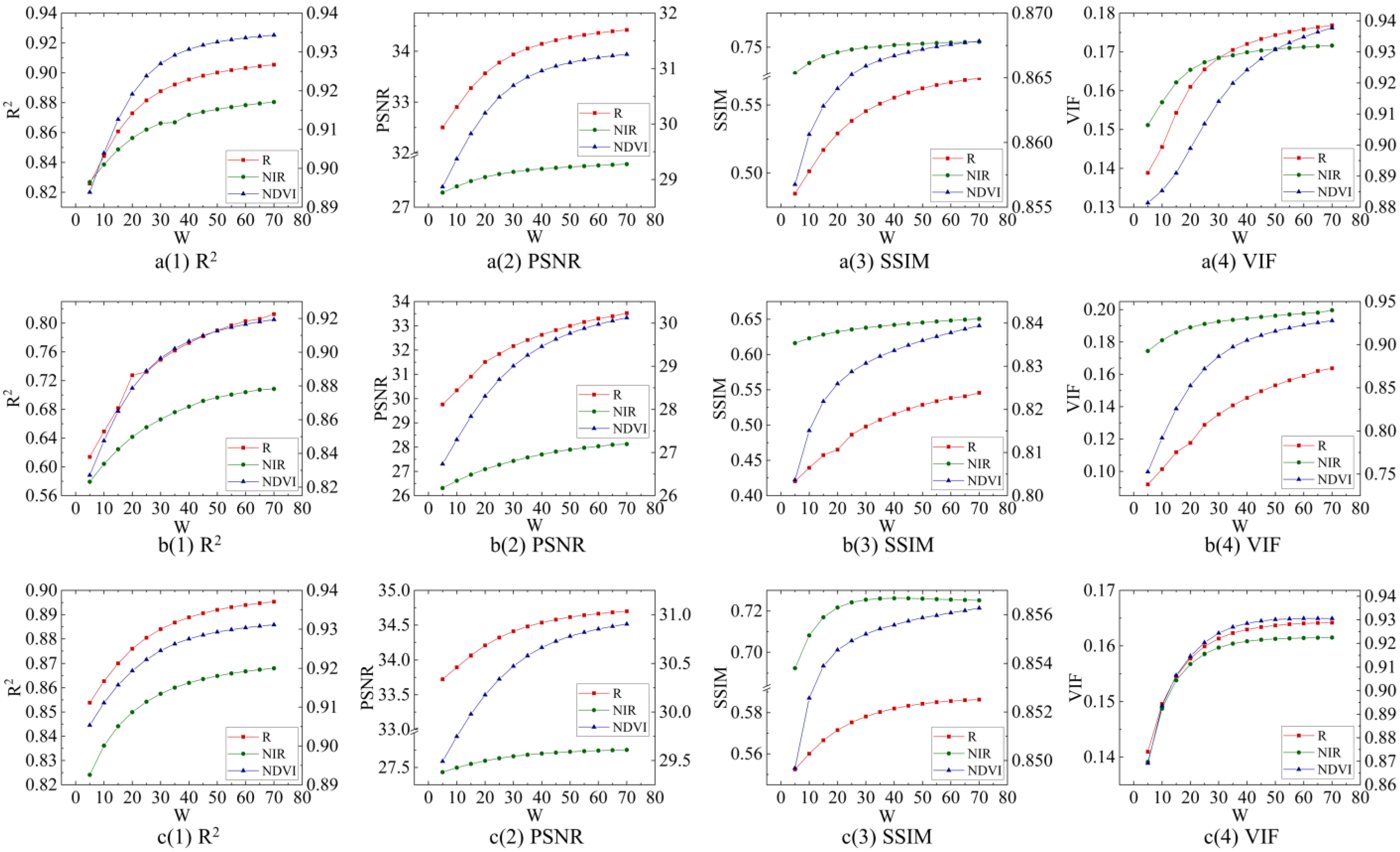
3.1.1. The Size of the Sliding Window

Figure 3 shows the PNSR, R², SSIM, and VIF results of the red band, near-red band, and NDVI data obtained from the fusion of each model with the corresponding real Sentinel-2 data using different sliding window values. In the figure, R and NIR represent the red and near-red bands, respectively, and W represents the sliding window size. In each subfigure, R and NIR correspond to the left y-axis and the NDVI to the right y-axis. By observing the data, it can be seen that the evaluation indexes corresponding to the three models first increased and then stabilized as the sliding window gradually became larger. For the STARFM, the PSNR of the fusion results stabilized when the sliding window edge length was greater than 45 pixels, at which point the PSNR values corresponding to the red and near-red bands and the NDVI were all greater than 27 dB, with the NDVI remaining above 31 dB. These values indicated that the distortion between the three images obtained from STARFM fusion and the real Sentinel-2 data was low, and the image quality was relatively good. Similar results were obtained for the ESTARFM and FSDAF model. The R² of the red band, near-red band, and NDVI obtained from the fusion of the three models did not change much after the sliding window edge length increased to 50 pixels. The results obtained from the ESTARFM corresponded to a relatively low R², where the R² of the red band never reached 0.85, and the R² of the near-red band was less than 0.72.

Table 3. Indicator values for each band of the three models using a window size of 70 pixels.

Method	Accuracy Indicators for the Different Bands
	R				NIR				NDVI
	PSNR	R2	SSIM	VIF	PSNR	R2	SSIM	VIF	PSNR	R2	SSIM	VIF
STRAFM	34.419	0.905	0.570	0.177	27.846	0.880	0.754	0.172	31.257	0.934	0.868	0.938
ESTRAFM	33.523	0.812	0.546	0.164	28.124	0.708	0.650	0.200	30.124	0.919	0.839	0.928
FSDAF	34.697	0.895	0.586	0.164	27.753	0.868	0.725	0.161	30.903	0.931	0.856	0.931

shows the accuracy information corresponding to each band of the three models using a sliding window size of 70 pixels. The ESTARFM had the lowest value of R² corresponding to the NDVI relative to the STARFM and FSDAF model. Accordingly, the results obtained from the ESTARFM corresponded to the SSIM values that were relatively low among the three models. The VIF results of the three models were roughly similar, and the results for the NDVI were much higher relative to the red band and near-red band VIF values.

Collectively, the good performance of the PSNR indicated that the three spatiotemporal fusion models were feasible for the fusion of Sentinel-2 and MODIS data in the TRHR, and the fusion results were indeed influenced by the sliding window size. A larger sliding window increased the corresponding model fusion time. After comprehensive consideration, the sliding window size of the STARFM, ESTARFM, and FSDAF model was selected to be 50 pixels. In addition, when studying the effect of the sliding window size, the selected number of similar images for the ESTARFM was 100, and in this case, the fusion effect of the ESTARFM was relatively weaker than the other two models. Since the accuracy of the ESTARFM was not only affected by the size of the sliding window, this paper further investigated the effect of the change in the number of similar images on the accuracy of the ESTARFM.

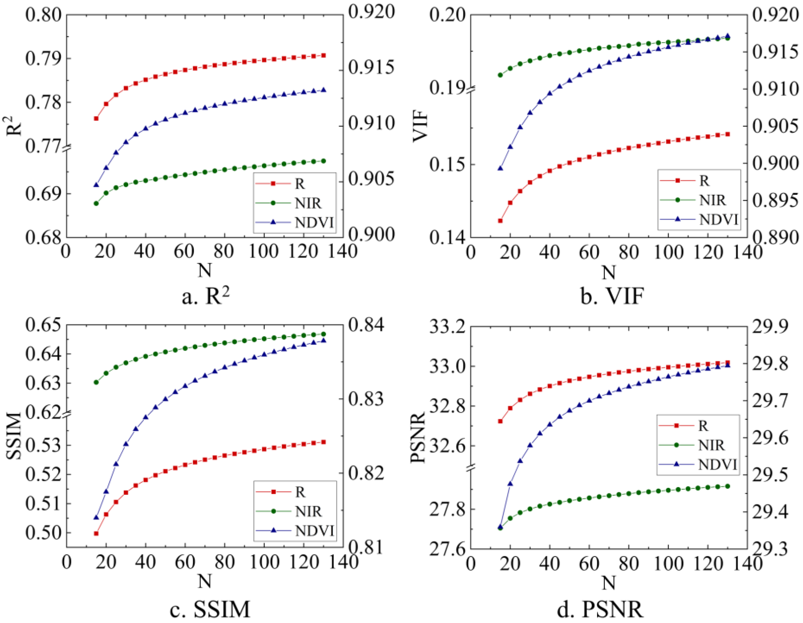
3.1.2. The Number of Similar Pixels

The experimental results for the number of similar pixels are shown in Figure 4. In the figure, R and NIR represent the red and near-red bands, respectively, and N represents the number of similar image elements. R and NIR correspond to the left y-axis and the NDVI corresponds to the right y-axis. With a sliding window size of 50 pixels and the number of similar pixels set between 15 to 130, the fusion accuracy of the ESTARFM was observed. The PNSR, R2, SSIM, and VIF all showed an increasing trend and then stabilized, with little subsequent change. In particular, when the number of similar elements was around 120, the ESTARFM fusion effect reached its optimum. However, comparing the accuracy evaluation indexes corresponding to its red and near-red bands and NDVI values, we found that its fusion effect was still weaker than that of the STARFM and FSDAF model.

In a comprehensive analysis, with suitable parameters, the fusion accuracy of the STARFM and FSDAF model in this study area was higher and the information retention was richer. The ESTARFM was more suitable for areas with fragmented plots and a strong landscape heterogeneity, while the feature types in this study area were relatively simple, with only vegetation, bare soil, snow/clouds, and four other major categories. The landscape heterogeneity did not vary much, and therefore its fusion effect in this study was relatively worse than that of the STARFM and FSDAF model consistent with previous studies. In addition, the ESTARFM required more input of high-quality data for fusion, and this limitation was significant for the present study area which was cloudy and rainy. It is recommended to use the STARFM or FSDAF model for the spatiotemporal fusion of Sentinel-2 and MODIS data in this experimental area, and the sliding window size W of these two models can be set to 50 pixels or more. As shown in

Table 4. Comparison of the temporal and spatial resolutions of the data before and after fusion.

	Experimental Data	Spatial Resolution (m)	Time Resolution (D)
Before fusion	Sentinel-2	10	5
	MODIS	250	<1
After fusion		10	<1

, the fused experimental data reached a temporal resolution of less than 1 day and a spatial resolution of 10 m, which can provide important support for constructing high-quality time series data and further studying the surface vegetation cover in the TRHR on a large scale and with a higher accuracy.

3.1.3. The Fusion Effect of the Comparison Experiment

The results of experiments I and II corresponding to the fusion effects of the STARFM and FSDAF model using the optimal parameters are shown in Figure 5. When comparing the experimental results, it was found that the similarity between the NDVI and the real NDVI obtained by both models using the two fusion methods was very high.

The NDVI images obtained from the model fusion were regressed against the actual images and the scatter plots were drawn (Figure 6). The R² of the regression coefficients of both the STARFM and FSDAF model in experiment II were greater than that of experiment I, and the values were both above 0.93. This indicated that performing the calculation of the vegetation index first, and then conducting the spatiotemporal fusion helped to obtain better data. Considering the fact that the normalized vegetation index can eliminate some of the radiometric errors in the calculation process, the results of this comparative experiment can be considered to be more in line with the pattern.

4. Discussion

The results of this paper showed that three models, the STARFM, ESTARFM, and FSDAF model, had better fusion results when applied to the experimental bands of the Sentinel-2 and MODIS data in a typical region of the TRHR under suitable parameter configuration conditions. Among them, the fusion accuracies of the STARFM and FSDAF model were higher. The experimental results showed that the accuracy of direct vegetation index data fusion was higher, and in-depth studies such as surface vegetation cover can be conducted on this basis. The existing studies mostly applied the fusion model to Landsat and MODIS data [34], and the study of grassland cover change and toxic weed invasion in the TRHR also focused on medium- and low-resolution remote sensing data [35]. In contrast, Sentinel-2 had a higher spatial resolution compared to Landsat data, and the accuracy of monitoring the surface vegetation cover and change was also higher. In the actual fusion process, the influence of different model parameter settings on the fusion effect was very important, and most of the current studies mainly used the default parameters proposed by the developers. Under the influence of the study areas with different surface complexities and different data sources, the parameter settings needed to be explored accordingly. In addition, in the application of a spatiotemporal fusion model for the study of the surface vegetation cover [36], there were those who performed the fusion after the waveform calculation, and those who calculated the vegetation index after the waveform fusion [37]. The different timing of the fusion also had an impact on the accuracy of the fusion results. This study discussed in detail the suitable fusion model and its corresponding parameter settings in a typical area of the TRHR, clarified the timing of vegetation index data fusion, and provided support for further studies on the surface vegetation cover in this study area.

Since the TRHR has a unique geographical environment and diverse types of grassland vegetation degradation, it was important to monitor and identify the surface vegetation on a large scale for the ecological evolution, biodiversity conservation, and sustainable development of grassland resources in the area. The identification and monitoring of large areas of grassland depend on remote sensing data with high spatial and temporal resolutions. This study explored the spatial and temporal fusion model and the corresponding parameter settings that were suitable for the area, which could effectively alleviate the limitations of the study caused by a single data source or interference from weather. Improving the temporal resolution of remote sensing images can support the detection of surface vegetation changes in the TRHR and improving the spatial resolution can improve the recognition accuracy of the grassland ecological community succession and toxic weed invasion in the TRHR. The results of the comparison experiments showed that the fusion based on the NDVI data products was also feasible for this region, which reduced the calculation time for the surface vegetation identification studies.

The three fusion methods selected in this study were classical and widely used methods. The experimental bands did not cover all the bands contained in the Sentinel-2 and MODIS data, and the existing spatiotemporal fusion models were thoroughly developed. Therefore, we can also expand the discussion on whether other models are more suitable for future research. Our next research direction is to explore the most suitable spatiotemporal fusion model and its optimal parameters in the TRHR, and subsequently construct a high spatiotemporal resolution time series data set, extract the surface phenology of the study area, and further study the spatial distribution and spatial and temporal evolution of toxic weeds and native dominant forbs in the area.

5. Conclusions

In this study, the applicability of the STARFM, ESTARFM, and FSDAF in the TRHR was analyzed by combining Sentinel-2 and MODIS data, and the results showed the following:

(1)

The accuracy of the spatiotemporal fusion models involved in this study was influenced by the parameters. With a gradual increase in the size of the sliding window, the fusion accuracy of all three models showed a trend of increasing first and then leveling off. Considering the influence of the size of the sliding window on the running time of the fusion model, the sliding window size was set to 50 pixels. For the ESTARFM, the fusion accuracy increased with an increase in the number of similar pixels and stabilized after the number of similar pixels became greater than 80 when the window size was constant.

(2)

According to the results of the study, compared to the ESTARFM, the STARFM and FSADF model had better fusion effects and higher accuracies. We recommend the use of the STARFM and FSDAF model for spatiotemporal fusion in this study area.

(3)

The comparison of the experimental results showed that the order of the fusion and calculation of the NDVI had an influence on the accuracy of the final vegetation index. The calculation of the vegetation index followed by the spatiotemporal integration produced a higher accuracy. In other words, it is possible to perform spatiotemporal data fusion directly on the vegetation index data products, which can simultaneously save time and obtain high-precision data.

References

- An, R.; Lu, C.; Wang, H.; Jiang, D.; Sun, M.; Jonathan Arthur Quaye, B. Remote Sensing Identification of Rangeland Degradation Using Hyperion Hyperspectral Image in a Typical Area for Three-River Headwater Region, Qinghai, China. Geomat. Inf. Sci. Wuhan Univ. 2018, 43, 399–405. [Google Scholar]
- Pan, L.; Xia, H.; Yang, J.; Niu, W.; Wang, R.; Song, H.; Guo, Y.; Quin, Y. Geoinformation, Mapping cropping intensity in Huaihe basin using phenology algorithm, all Sentinel-2 and Landsat images in Google Earth Engine. Int. J. Appl. Earth Obs. Geoinf. 2021, 102, 102376. [Google Scholar]
- Raffini, F.; Bertorelle, G.; Biello, R.; D’Urso, G.; Russo, D.; Bosso, L.J.S. Supplementary Materials–From Nucleotides to Satellite Imagery: Approaches to Identify and Manage the Invasive Pathogen Xylella fastidiosa and Its Insect Vectors in Europe. Sustainability 2020, 12, 4508. [Google Scholar] [CrossRef]
- Huang, B.; Jiang, X. An enhanced unmixing model for spatiotemporal image fusion. J. Remote Sens. 2021, 25, 241–250. [Google Scholar]
- Hu, Y.F.; Wang, H.; Niu, X.Y.; Shao, W.; Yang, Y.C. Comparative Analysis and Comprehensive Trade-Off of Four Spatiotemporal Fusion Models for NDVI Generation. Remote Sens. 2022, 14, 5996. [Google Scholar] [CrossRef]
- Zhu, X.; Helmer, E.H.; Gao, F.; Liu, D.; Chen, J.; Lefsky, M.A. A flexible spatiotemporal method for fusing satellite images with different resolutions. Remote Sens. Environ. 2016, 172, 165–177. [Google Scholar] [CrossRef]
- Gao, F.; Masek, J.; Schwaller, M.; Hall, F. On the blending of the Landsat and MODIS surface reflectance: Predicting daily Landsat surface reflectance. IEEE Trans. Geosci. Remote Sens. 2006, 44, 2207–2218. [Google Scholar]
- Zhu, X.; Chen, J.; Gao, F.; Chen, X.; Masek, J.G. An enhanced spatial and temporal adaptive reflectance fusion model for complex heterogeneous regions. Remote Sens. Environ. 2010, 114, 2610–2623. [Google Scholar] [CrossRef]
- Wu, M.; Niu, Z.; Wang, C. Assessing the Accuracy of Spatial and Temporal Image Fusion Model of Complex area in South China. J. Geo-Inf. Sci. 2014, 16, 776–783. [Google Scholar]
- He, X.; Jing, Y.S.; Gu, X.H.; Huang, W.J. A Province-Scale Maize Yield Estimation Method Based on TM and Modis Time-Series Interpolation. Sens. Lett. 2010, 8, 2–5. [Google Scholar] [CrossRef]
- Wu, M.; Niu, Z.; Wang, C.; Wu, C.; Wang, L. Use of MODIS and Landsat time series data to generate high-resolution temporal synthetic Landsat data using a spatial and temporal reflectance fusion model. J. Appl. Remote Sens. 2012, 6, 63507. [Google Scholar]
- Shi, Y.-C.; Yang, G.-J.; Li, X.-C.; Song, J.; Wang, J.-H.; Wang, J.-D. Intercomparison of the different fusion methods for generating high spatial-temporal resolution data. J. Infrared Millim. Waves 2015, 34, 92–99. [Google Scholar]
- Ibn El Hobyb, A.; Radgui, A.; Tamtaoui, A.; Er-Raji, A.; El Hadani, D.; Merdas, M.; Smiej, F.M. Evaluation of spatiotemporal fusion methods for high resolution daily NDVI prediction. In Proceedings of the 5th International Conference on Multimedia Computing and Systems (ICMCS), Marrakech, Morocco, 29 September–1 October 2016; pp. 121–126. [Google Scholar]
- Jun, L.I.; Yunfei, L.I.; Lin, H.E.; Chen, J.; Plaza, A. Spatio-temporal fusion for remote sensing data:an overview and new benchmark. Sci. China Inf. Sci. 2020, 63, 7–23. [Google Scholar]
- Zhang, K.; Wei, W.; Zhou, J.; Yin, L.; Xia, J. Spatial-temporal Evolution Characteristics and Mechanism of ”Three-Function Space” in the Three-Rivers Headwaters’ Region from 1992 to 2020. J. Geo-Inf. Sci. 2022, 24, 1755–1770. [Google Scholar]
- Zhang, Y.; Zhang, C.; Wang, Z.; Yang, Y.; Zhang, Y.; Li, J.; An, R. Quantitative assessment of relative roles of climate change and human activities on grassland net primary productivity in the Three-River Source Region, China. Acta Prataculturae Sinica 2017, 26, 1–14. [Google Scholar]
- Guan, Q.; Ding, M.; Zhang, H. Spatiotemporal Variation of Spring Phenology in Alpine Grassland and Response to Climate Changes on the Qinghai-Tibet, China. Mt. Res. 2019, 37, 639–648. [Google Scholar]
- Claverie, M.; Ju, J.; Masek, J.G.; Dungan, J.L.; Vermote, E.F.; Roger, J.-C.; Skakun, S.V.; Justice, C. The Harmonized Landsat and Sentinel-2 surface reflectance data set. Remote Sens. Environ. 2018, 219, 145–161. [Google Scholar] [CrossRef]
- Zhao, Q.; Ding, J.; Han, L.; Jin, X.; Hao, J. Exploring the application of MODIS and Landsat spatiotemporal fusion images in soil salinization: A case of Ugan River-Kuqa River Delta Oasis. Arid. Land Geogr. 2022, 45, 1155–1164. [Google Scholar]
- Yin, X.; Zhu, H.; Gao, J.; Gao, J.; Guo, L.; Gou, Z. NPP Simulation of Agricultural and Pastoral Areas Based on Landsat and MODIS Data Fusion. Trans. Chin. Soc. Agric. Mach. 2020, 51, 163–170. [Google Scholar]
- Ge, Y.; Li, Y.; Sun, K.; Li, D.; Chen, Y.; Li, X. Two-way fusion experiment of Landsat and MODIS satellite data. Sci. Surv. Mapp. 2019, 44, 107–114. [Google Scholar]
- Guan, Q.; Ding, M.; Zhang, H.; Wang, P. Analysis of Applicability about ESTARFM in the Middle-Lower Yangtze Plain. J. Geo-Inf. Sci. 2021, 23, 1118–1130. [Google Scholar]
- Li, S.H.; Yu, D.Y.; Huang, T.; Hao, R.F. Identifying priority conservation areas based on comprehensive consideration of biodiversity and ecosystem services in the Three-River Headwaters Region, China. J. Clean Prod. 2022, 359, 13. [Google Scholar] [CrossRef]
- Wei, X.Y.; Mao, X.F.; Wang, W.Y.; Tao, Y.Q.; Tao, Z.F.; Wu, Y.; Ling, J.K. Measuring the Effectiveness of Four Restoration Technologies Applied in a Degraded Alpine Swamp Meadow in the Qinghai-Tibet Plateau, China. J. Environ. Account. Manag. 2021, 9, 59–74. [Google Scholar] [CrossRef]
- Zhou, W.; Li, H.; Shi, P.; Xie, L.; Yang, H. Spectral Characteristics of Vegetation of Poisonous Weed Degraded Grassland in the ”Three-River Headwaters” Region. J. Geo-Inf. Sci. 2020, 22, 1735–1742. [Google Scholar]
- Lei, C.; Meng, X.; Shao, F. Spatio-temporal fusion quality evaluation based on Point-Line-Planeaspects. J. Remote Sens. 2021, 25, 791–802. [Google Scholar]
- Wang, Z.; Bovik, A.C.; Sheikh, H.R.; Simoncelli, E.P. Image quality assessment: From error visibility to structural similarity. IEEE Trans. Image Process. 2004, 13, 600–612. [Google Scholar] [CrossRef]
- Sheikh, H.R.; Bovik, A.C. Image information and visual quality. IEEE Trans. Image Process. 2006, 15, 430–444. [Google Scholar] [CrossRef]
- Li, W.; Xu, J.; Yao, Y.; Zhang, Z. Temporal and Spatial Changes in the Vegetation Cover (NDVI) in the Three-River Headwater Region, Tibetan Plateau, China under Global Warming. Mt. Res. 2021, 39, 473–482. [Google Scholar]
- Sun, X.P.; Xiao, Y. Vegetation Growth Trends of Grasslands and Impact Factors in the Three Rivers Headwater Region. Land 2022, 11, 2201. [Google Scholar] [CrossRef]
- Hu, Y.; Dao, R.; Hu, Y. Vegetation Change and Driving Factors: Contribution Analysis in the Loess Plateau of China during 2000-2015. Sustainability 2019, 11, 1320. [Google Scholar] [CrossRef]
- Liu, S.; Sun, Y.; Zhao, H.; Liu, Y.; Li, M. Grassland dynamics and their driving factors associated with ecological construction projects in the Three-River Headwaters Region based on multi-source data. Acta Ecol. Sin. 2021, 41, 3865–3877. [Google Scholar]
- Gao, S.; Dong, G.; Jiang, X.; Nie, T.; Guo, X.; Dang, S. Analysis of Vegetation Coverage Changes and Natural Driving Factors in the Three-River Headwaters Region Based on Geographical Detector. Res. Soil Water Conserv. 2022, 29, 336–343. [Google Scholar]
- Ruan, Y.; Ruan, B.; Zhang, X.; Ao, Z.; Xin, Q.; Sun, Y.; Jing, F. Toward 30 m Fine-Resolution Land Surface Phenology Mapping at a Large Scale Using Spatiotemporal Fusion of MODIS and Landsat Data. Sustainability 2023, 15, 3365. [Google Scholar] [CrossRef]
- Sun, Q.; Liu, W.; Gao, Y.; Li, J.; Yang, C.J.S. Spatiotemporal Variation and Climate Influence Factors of Vegetation Ecological Quality in the Sanjiangyuan National Park. Sustainability 2020, 12, 6634. [Google Scholar] [CrossRef]
- Lu, Y.; Wu, P.; Ma, X.; Li, X.J.E.M. Assessment, Detection and prediction of land use/land cover change using spatiotemporal data fusion and the Cellular Automata–Markov model. Environ. Monit. Assess. 2019, 191, 1–19. [Google Scholar] [CrossRef]
- Li, S.; Zhang, W.; Yang, S. Intelligence fusion method research of multisource high-resolution remote sensing images. J. Remote Sens. 2017, 21, 415–424. [Google Scholar]