Response of Fish Habitat Quality to Weir Distribution Change in Mountainous River Based on the Two-Dimensional Habitat Suitability Model

Abstract

Weirs are often constructed on mountainous rivers because of their low construction costs and their ability to provide irrigation and facilitate landscaping, yet there is little research on how fish habitat quality in mountainous rivers responds to weir distribution. This study categorized the distribution characteristics of weirs on typical reaches according to their sinuosity and calculated the corresponding habitat suitability index (HSI) and weighted usable area (WUA) under various discharge conditions using a coupled MIKE21 and habitat suitability model. Then, the relationship between the distribution characteristics of weirs and the quality of fish habitats under different discharge conditions was analyzed. The results show that weirs in mountainous rivers can affect the habitat suitability of the rivers, but this effect is closely related to discharge conditions and layout mainly because the key hydraulic factors that determine habitat quality for different sinuous reaches vary under different discharge conditions. This study found that in high-sinuosity rivers with high discharge conditions, water depth is the key factor determining the quality of fish habitats, so weirs can improve habitat quality by improving the suitability of downstream water depth. However, in other conditions, velocity is the key factor determining habitat quality, in which case weirs cannot improve habitat quality and can even degrade it. Therefore, other methods of improving velocity are needed to enhance habitat quality. The results of this study provide a reference for the protection of fish habitats in mountainous river channels and the determination of suitable locations for weir construction.

1. Introduction

A habitat is the place where creatures live, and its quality reflects the ability of the environment to provide ample resources and conditions for a population to persist and reproduce [1]. Fish constitute the most populous community in aquatic ecosystems, so their habitat quality is essential to biodiversity conservation and aquatic functions in many areas [2]. However, many hydraulic projects alter the quality of fish habitats. Among these hydraulic projects, the impact of weirs on fish habitats in rivers has been widely debated. Many researchers argue that the construction of weirs leads to a decrease in fish habitat quality. This is due to factors such as the upstream storage of water in a reservoir, which increases the depth of a river and thus decreases its discharge speed [3], changes its water temperature [4], and alters the hydraulic environment such that is unsuitable for fish survival. The implementation of weirs also leads to changes in the longitudinal and lateral flow behavior and connectivity of a river [5] and hinders the migration of migratory fish [6,7], all of which contribute to a reduction in fish populations [8]. Therefore, many studies currently propose improving fish habitat quality by removing weirs. Research has shown that when weirs are removed, not only do the spawning success rate and fry survival rate of fish increase [9], but the fish habitat quality also increases significantly for all life stages and discharge conditions [10,11,12]. However, the spatial and temporal ecological impacts of weir removal are significant [13]. Nagayama et al. [14] indicate that long-term assessments are needed to accurately determine the effects of weir removal on habitat quality. However, due to the complexity of long-term assessments, most current studies do not conduct long-term assessments of biophysical responses before and after weir removal [15]. Furthermore, studies have demonstrated that weirs, as low-head structures, can also improve fish habitat quality under high-discharge conditions [16,17]. The use of various types of weirs or other engineering measures can also improve habitat quality by altering hydraulic conditions [18,19,20].

Mountain rivers exhibit great variability in hydrological conditions, elevation, and morphology [21]. Therefore, the construction of weirs at these locations can be utilized for multiple functions, including power generation, flood control, and irrigation. Additionally, the high degree of morphological variability in the rivers in such regions has contributed to an increase in meandering reaches. Field investigations have found that there are more ecological diversity indicators of meandering reaches than those of straight reaches. The higher the sinuosity of the meandering river, the more complex the river channel’s shape and the relatively higher the level of ecological stability of the river channel [22]. Therefore, many studies have shown that restoring meanders is an effective way to restore river habitats [23,24,25]. Meandering rivers are mainly classified based on their sinuosity. There are two commonly used sinuosity classifications: Lepold et al. [26] define rivers with sinuosity less than 1.3 as low-sinuosity rivers and those with sinuosity greater than 1.3 as high-sinuosity rivers. Rust [27] uses 1.5 as the line between high- and low-sinuosity rivers. Discharge is also critical to the functional role of weirs and the habitat quality of meandering rivers. For meandering rivers, habitat quality responds differently to discharge conditions for reaches with different sinuosity [28,29]. The distribution of fish habitats under normal discharge conditions differs from that under flood discharge conditions [30]. For weirs, lower discharge results in shallower depths on the weir crest, leading to a reduction in some of the behavioral stimuli (such as speed, presence at depth, etc.) required for fish to pass through a weir [31]. Therefore, it is essential to grasp the effects of weirs on fish habitat quality in rivers with different sinuosity levels under different discharge conditions in order to clarify the ecological effects of weirs.

This study selected the Lingshan River, which is situated in a mountainous area, as its study area. Through field investigations, the distributional characteristics of weirs in typical reaches were classified according to their sinuosity. The target fish species, namely, the four major Chinese carp species, were used to simulate habitats through numerical modeling. This study primarily aimed to (1) classify the distribution characteristics of weirs in the Lingshan River based on sinuosity; (2) explore the impacts of weirs and sinuosity on fish habitat quality; and (3) identify the key factors affecting habitat quality under different conditions.

2. Materials and Methods

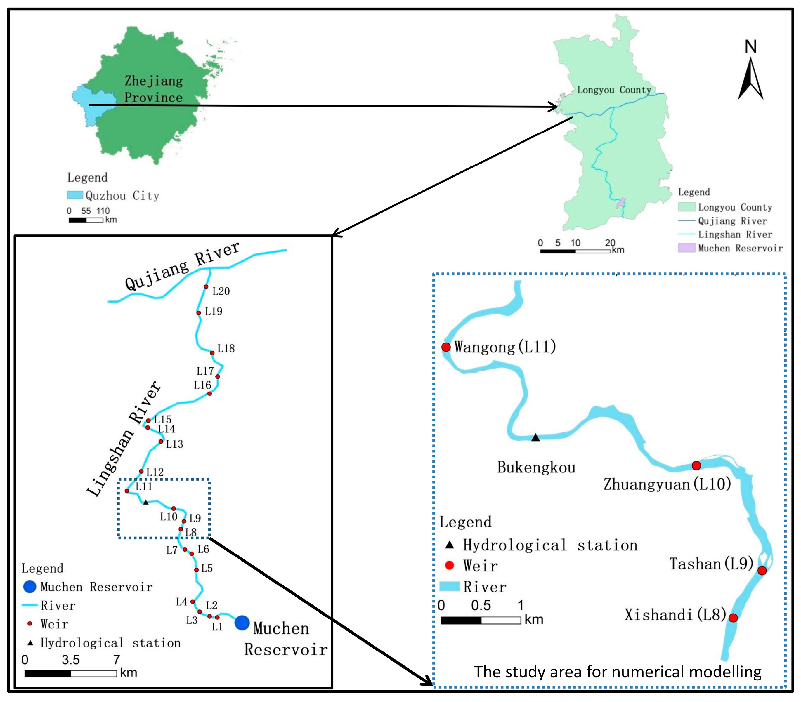
2.1. Study Area

The Lingshan River is located in Quzhou City, Zhejiang Province, China, between latitudes 28°47′ N–29°03′ N and longitudes 119°8′ E–119°12′ E. It is a tributary of the Qujiang River and is dominated by mountains with altitudes ranging from 33 to 1442 m above sea level, with an average slope of 2.45‰. The total length of the river is 90.6 km, and its drainage area is 726.9 km². The main climate type in the Lingshan River is subtropical monsoon, which is characterized by four distinct seasons. The area’s mean annual rainfall is 1666 mm, and 45.2% of its total rainfall occurs from March to June. In 2008, the Muchen Reservoir was built in the upper reaches of the Lingshan River, with a catchment area of 397 km² and a total storage capacity of 125.71 million m³. To meet domestic water, irrigation, landscape ecology, and hydropower requirements, 20 weirs were constructed along the Muchen reservoir to the confluence of the Qujiang River with the Lingshan River. The Lingshan River contains 9 orders, 12 families, and 49 species of fish, including 8 subfamilies and 33 species of Cyprinidae. Through field investigation and the use of relevant materials, this study determined the target fishes to be the four major Chinese carp and selected the spawning period of March to July for assessment of the river’s habitat quality since the number of fish populations depends on the availability and quality of spawning period habitat [32].

Based on field research, we selected a reach with multiple meandering sub-reaches and weirs for our research (Figure 1). The studied reach extends from upstream of the Xishandi weir to downstream of the Wangong weir, amounting to a region that is about 8.4 km long. This reach has multiple meandering sub-reaches; four weirs, namely, Xishandi Weir, Tashan Weir, Zhuangyuan Weir, and Wangong Weir; and one hydrological station, i.e., Bukengkou (

Table 1. Geographic coordinates, heights, and widths of the weirs.

Weirs	Latitudes	Longitudes	Height (m)	Width (m)
Xishandi	28°52′32″ N	119°9′39″ E	1.8	2.0
Tashan	28°52′50″ N	119°9′53″ E	1.9	2.0
Zhuangyuan	28°53′30″ N	119°9′24″ E	1.7	2.0
Wangong	28°54′16″ N	119°7′25″ E	2.0	2.1

). These four weirs are basically similar in shape, height, and width. The discharge of the Bukengkou hydrological station from March to July ranges from 28.24 m³/s to 60.48 m³/s, and its average discharge is 38.92 m³/s.

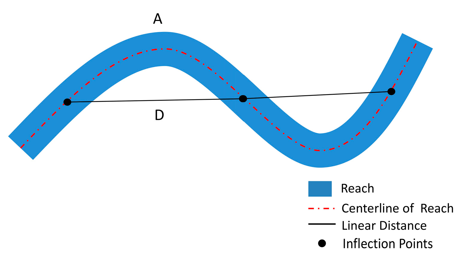
2.2. Calculation of River Sinuosity

In this paper, the studied river’s morphology is classified according to its sinuosity. Sinuosity was calculated using the inflection sinuosity method, which involves dividing the length of the centerline by the distance between adjacent inflection points [33]. Based on Leopold’s classification method and field observations, a reach with a sinuosity level less than 1.3 was termed a low-sinuosity reach (LSR), a reach with a sinuosity level greater than 1.3 and less than 1.6 was termed a medium-sinuosity reach (MSR), and a reach with a sinuosity level greater than 1.6 was termed a high-sinuosity reach (HSR). A reach without noticeable bends was termed a straight reach (SR).

$$Si=\frac{A}{D}$$

(1)

In the above equation, $Si$ is sinuosity, while $A$ and $D$ are the length measured along the reach’s centerline and the linear distance between the contiguous inflection points, respectively (Figure 2).

2.3. Hydrodynamic Model

2.3.1. Governing Equation

The Mike 21 FM model used in this study is a two-dimensional numerical simulation model based on fluid dynamics. The Mike21 FM water environment model mainly consists of a hydrodynamic module and a water ecology laboratory simulation. Hydrodynamic module simulates the hydraulic characteristics of the reach under different discharge conditions, including factors such as flow velocity and water depth. The MIKE 21 FM model is based on the numerical solution of the two-dimensional shallow water equation, which integrates the incompressible Reynolds Averaged Navier–Stokes equation with respect to water depth. The numerical method employed is the finite volume method in a grid, which divides the continuum into triangular and quadrangular non-overlapping grids and calculates the hydraulic characteristics of each grid [34].

(1)

Continuity equation:

$$\frac{\partial h}{\partial t}+\frac{\partial h\overline{u}}{\partial x}+\frac{\partial h\overline{v}}{\partial y}=hS$$

(2)

(2)

Momentum equation:

X-direction momentum:

$$\frac{\partial h\overline{u}}{\partial t}+\frac{\partial h{\overline{u}}^2}{\partial x}+\frac{\partial h\overline{vu}}{\partial y}=f\overline{v}h-gh\frac{\partial \eta }{\partial x}-\frac{h}{{\rho }_0}\frac{\partial P_a}{\partial x}-$$

$$\frac{g{h}^2}{ 2{\rho }_0}\frac{\partial \rho }{\partial x}+\frac{{\tau }_{sx}}{{\rho }_0}-\frac{{\tau }_{bx}}{{\rho }_0}-\frac{1}{{\rho }_0}\left(\frac{\partial s_{xy}}{\partial y}+\frac{\partial s_{xx}}{\partial x}\right)$$

(3)

$$+\frac{\partial }{\partial x}\left(h{T}_{xx}\right)+\frac{\partial }{\partial y}\left(h{T}_{xy}\right)+h{u}_s$$

Y-direction momentum:

$$\frac{\partial h\overline{v}}{\partial t}+\frac{\partial h{\overline{v}}^2}{\partial y}+\frac{\partial h\overline{uv}}{\partial x}=f\overline{u}h-gh\frac{\partial \eta }{\partial y}-\frac{h}{{\rho }_0}\frac{\partial P_a}{\partial y}-$$

$$\frac{g{h}^2}{ 2{\rho }_0}\frac{\partial \rho }{\partial y}+\frac{{\tau }_{sy}}{{\rho }_0}-\frac{{\tau }_{by}}{{\rho }_0}-\frac{1}{{\rho }_0}\left(\frac{\partial s_{yx}}{\partial x}+\frac{\partial s_{yy}}{\partial y}\right)$$

(4)

$$+\frac{\partial }{\partial x}\left(h{T}_{xy}\right)+\frac{\partial }{\partial y}\left(h{T}_{yy}\right)+h{v}_{s}S$$

where $t$ is the time in s; $\eta$ is the elevation of the river bottom in m; $d$ is depth of water in m; $h$ is the total water depth in m, where $h$= $\eta +d$; $\mathrm{u}$ and $v$ are the velocity components in the x and y direction in m/s; $S$ is the source in m³/s; $f$ is the Coriolis parameter in s⁻¹, where $f=2\omega \mathit{sin}\phi$, for which $\omega$ is the angular rate of revolution and $\phi$ is the geographic latitude; $g$ is the gravitational acceleration in m/s²; $P_a$ is atmospheric pressure in N/m²; $\rho$ is the density of water in kg/m³; ${\rho }_0$ is the reference density of water in kg/m³; $s_{xy}, s_{xx},s_{yx}$, and $s_{yy}$ are components of the radiation stress tensor in N/m; $f\overline{u}$ and $f\overline{v}$ are acceleration components of the earth’s rotation in m/s²; $v_s$ and $u_s$ are the velocity with which the water is discharged into the ambient water in m/s; $T_{ij}$ is the lateral stress in N/m²; ${\tau }_{sy}$ and ${\tau }_{sx}$ are the surface stress in N/m²; ${\tau }_{by}$ and ${\tau }_{bx}$ are the bottom stress in N/m².

2.3.2. Boundary Condition

During the simulation, the upstream boundary conditions were set using discharge conditions, and the downstream boundary conditions were set using water depth conditions. These settings can render a model more stable and convergent [35]. In the simulation, the discharge was first set as the upstream boundary; the discharge condition was set according to the March to July discharge (from 28.24 m³/s to 60.48 m³/s) of the hydrological station, which was set to range from 20 m³/s to 70 m³/s, and the simulation was set every 10 m³/s. Then, the downstream boundary conditions were set based on the measured water level downstream corresponding to the related discharge.

2.3.3. Calibration and Validation

Model accuracy is crucial in this study, so the model requires calibration and validation. The purpose of calibration is to determine the roughness of a model. Roughness significantly impacts results of a simulation, so it is important to select a suitable roughness value for a model. The purpose of validation is to ensure that the model can effectively and truly simulate the hydraulic characteristics of the studied river. Thus, the data in different periods were selected for calibration and verification; then, the Nash–Sutcliffe efficiency coefficient ($E_{ns}$) and $R^2$ were used to judge the quality of calibration and verification [36,37]

$$E_{ns}=1-\frac{{{\displaystyle \sum }}_{t=1}^T{\left(Q_o^t-Q_m^t\right)}^2}{{{\displaystyle \sum }}_{t=1}^T{\left(Q_o^t-\overline{Q_O}\right)}^2}$$

(5)

$$R^2={\displaystyle \sum }_{t=1}^T{\left(Q_o^t-Q_m^t\right)}^2$$

(6)

where $Q_o^t$ is the t-th observed value; $Q_m^t$ is the t-th simulated value; $\overline{Q_O}$ is the average of the values observed. An $E_{ns}$ greater than 0.5 indicates that a model is acceptable [38].

Model calibration involved setting an initial roughness, inputting the discharge measured upstream and the water depth measured downstream, and comparing the simulated data with the measured data from Bukengkou Hydrologic Station. If the error was significant, the roughness value was adjusted, and the simulation was repeated until the error was within an acceptable range. Consequently, the roughness value could be considered to correspond to the actual roughness of the river.

We performed model calibration using simulated and measured water depths in BKK from 1 May 2017 to 10 May 2017. Different roughness values were chosen to calculate $R^2$ and $E_{ns}$ values. When the roughness value was set to 0.033, the results, as shown in

Table 2. Comparison of the measured and simulated values of water depth.

	Model Calibration			Model Validation
	Water Depth (m)			Water Depth (m)
Date	Observed Value	Simulated Value	Date	Observed Value	Simulated Value
1 May 2017	1.36	1.35	1 May 2018	1.33	1.33
2 May 2017	1.27	1.28	2 May 2018	1.22	1.20
3 May 2017	1.37	1.35	3 May 2018	1.30	1.31
4 May 2017	1.40	1.38	4 May 2018	1.18	1.20
5 May 2017	1.36	1.33	5 May 2018	1.31	1.33
6 May 2017	1.38	1.40	6 May 2018	1.29	1.30
7 May 2017	1.28	1.30	7 May 2018	1.44	1.42
8 May 2017	1.35	1.33	8 May 2018	1.58	1.55
9 May 2017	1.33	1.33	9 May 2018	1.40	1.41
10 May 2017	1.37	1.40	10 May 2018	1.35	1.33
R2	0.004			0.003
$E_{ns}$	0.824			0.972

, yielded an $R^2$ value of 0.004 and an $E_{ns}$ value of 0.824. These results indicate that when the roughness value is 0.033, the model closely represents the actual roughness conditions of the river. The simulated and measured water depths in the BKK from 1 May 2018 to 10 May 2018, were compared to validate the model. As shown in Table 2, the $R^2$ is 0.003 and the $E_{ns}$ is 0.972. These results indicate that the hydraulic model used in this paper accurately reflects the hydrodynamic parameters of the studied river.

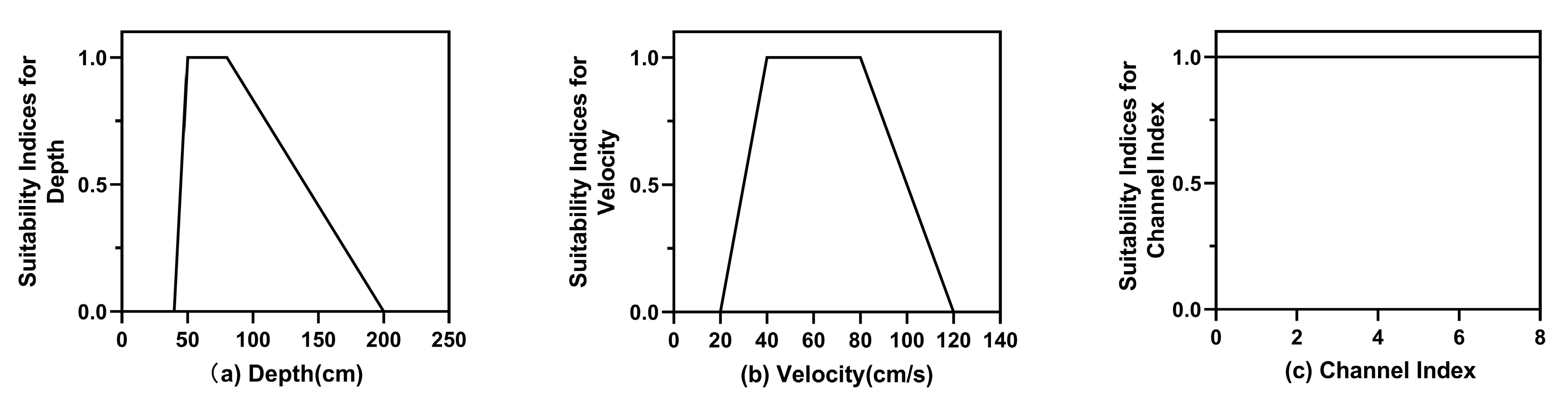
2.4. Habitat Suitability Model

A habitat suitability model is used quantify a target fish’s preference for different physical variables, such as velocity, water depth, and the type of substrate, at a specific life stage by converting them into indicators. A habitat model typically uses the habitat suitability index (HSI) to evaluate the habitat preferences of the target species. HSI was initially proposed by the U.S. Fish and Wildlife Service in their Habitat Evaluation Procedures (HEP) [39].

In order to calculate HSI, the first step is to construct habitat suitability curves, such as velocity suitability curve, depth suitability curve, and channel index suitability curve. These curves are used to quantitatively describe the suitability of a habitat for a given species, with values ranging from 0 to 1, where 0 denotes total unsuitability and 1 denotes complete suitability; the larger the value, the better the suitability. According to a relevant investigation, the optimum velocity ranges from 40 to 80 cm/s, while the suitable velocity ranges from 20 to 120 cm/s. The optimum water depth ranges from 50 to 80 cm, and the suitable water depth ranges from 40 to 200 cm [40]. Since the channel substrate or cover in the studied river has not been significantly disturbed, the channel index of each grid in the studied river is considered to be 1 (Figure 3).

The second step is to calculate the composite suitability index because fish select suitable combinations of velocity, water depth, and channel indices. This composite suitability can be calculated through various methods, such as arithmetical mean, geometric mean, minimum factor, weighted summation, or weighted product [41,42]. In this paper, the habitat suitability index (HSI) is calculated using the arithmetic mean:

$$HSI=V_i\times D_i\times C_i$$

(7)

where $V_i$ is the velocity suitability index; $D_i$ is the depth suitability index; $C_i$ is the suitability index of the channel index.

When HSI is less than 0.5, the level of suitability is poor; when HSI is greater than 0.5 and less than 0.8, the suitability is potentially suitable; and when HSI is greater than 0.8, the suitability is ideal [43]. In this paper, both $D_i$ and $V_i$ were analyzed based on the HSI classification method and categorized as poor, potentially suitable, and ideal.

To evaluate habitat quality, this paper also uses the Weighted Usable Area (WUA), the percentage of WUA with respect to the total area ($P_T$), and the difference in $P_T$ between different numbers of weirs ($D{P}_T$). While the HSI reflects the habitat quality of a single grid, the Weighted Usable Area (WUA) can reflect the habitat quality of the whole research region [44]. The WUA is calculated by summing all products of the area of each grid and their HSI values [45,46]. For the reach studied herein, 500 m upstream and 500 m downstream of the bend vertex are selected to calculate the WUA. $P_T$ can be used to compare the habitat quality of different reaches.

$$WUA={\displaystyle \sum }_{i=1}^M(A_i\times HS{I}_i)$$

(8)

In the equation above, $A_i$ is the area of the i-th grid; $HS{I}_i$ is the composite suitability index of the i-th grid; M is the total number of grid.

$$P_T=\frac{WUA}{TA}\times 100\%$$

(9)

In the equation above, $TA$ is the sum of the areas of all grids in the reach.

$$D{P}_T=P_{AT}-P_{BT}$$

(10)

In the equation above, $P_{AT}$ is the $P_T$ under A conditions; $P_{BT}$ is the $P_T$ under B conditions; A and B denote different numbers of weirs.

3. Results

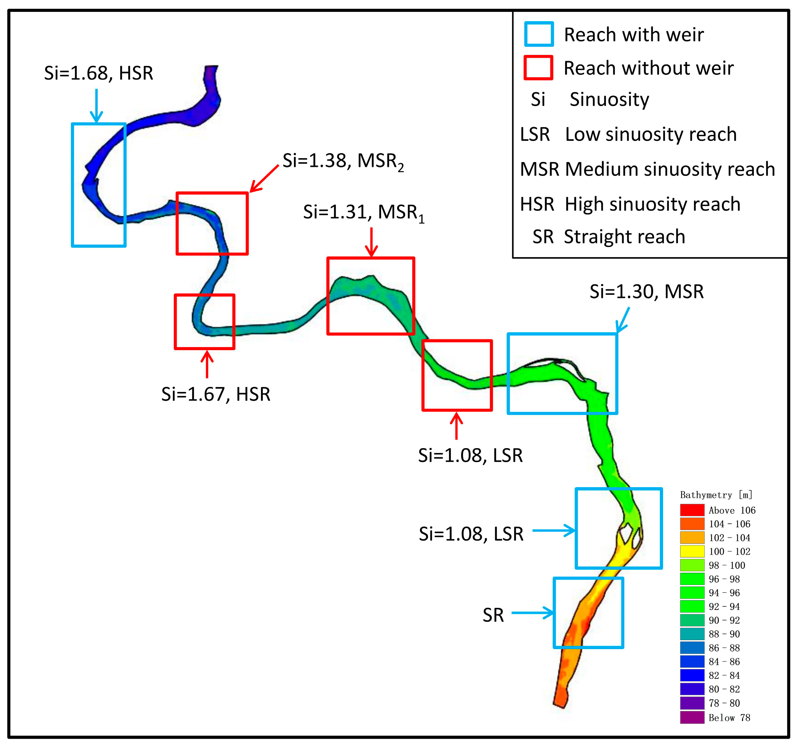
3.1. Distribution Characteristics of Weir

This study analyzes seven sinuosity reaches and one straight reach. After calculating the sinuosity of the seven sinuosity reaches, the morphologies of these seven sinuosity reaches were divided, including two high-sinuosity reaches, two low-sinuosity reaches, and three medium-sinuosity reaches (Figure 4). There is a significant difference between the values of sinuosity, ranging from 1.08 to 1.68. The weirs are distributed along SR, LSR, MSR, and HSR. Therefore, the distribution characteristics of the weirs can be summarized as follows: a low-sinuosity reach with a weir (LSR_w), a medium-sinuosity reach with a weir (MSR_w), and a high-sinuosity reach with a weir (HSR_w.). The HSR_w and the LSR_w each contain only one reach, while the MSR_w has two reaches. Therefore, we have selected MSR₁, which has a comparable sinuosity to an MSR, as the representative reach for further investigation in subsequent analyses.

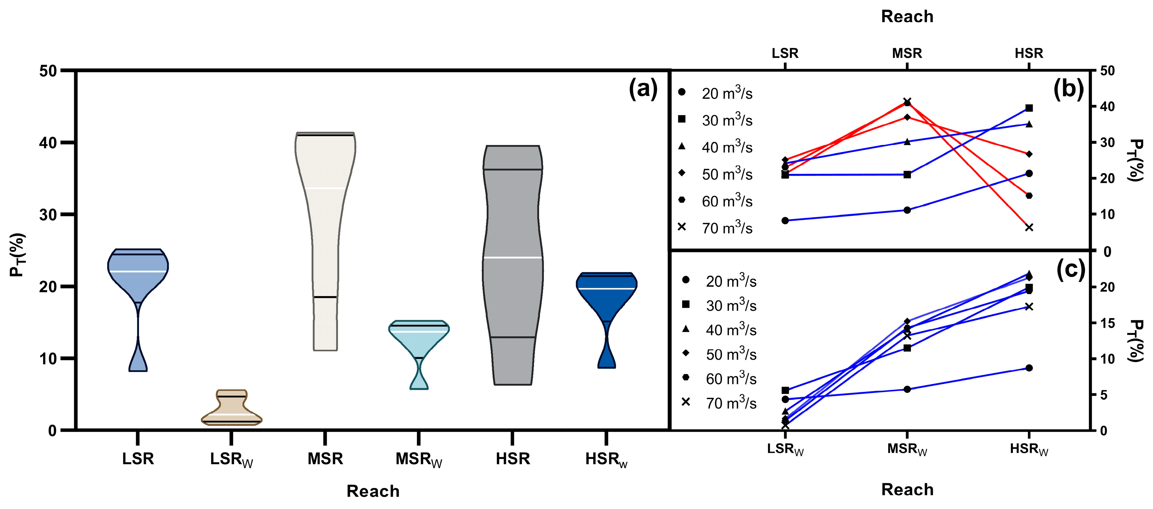
3.2. The Change of Fish Habitat Quality in Different Reaches

3.2.1. The Change in $P_T$

The results in Figure 5a illustrate that in the category without weirs, as sinuosity increases, $P_T$ varies more evenly and stably with changes in discharge. However, this phenomenon is not observed in the category with weirs. Additionally, it can be observed that within the same sinuosity level, the average $P_T$ of the weirs group is significantly lower than that of the no-weirs group. Figure 5b depicts the relationship between $P_T$ and sinuosity for six discharges ranging from 20 m³/s to 70 m³/s in the no-weirs category. It is evident that $P_T$ increases with sinuosity at discharges of 20 m³/s, 30 m³/s, and 40 m³/s, attaining its highest value at HSR. In contrast, at discharges of 50 m³/s, 60 m³/s, and 70 m³/s, $P_T$ initially increases with sinuosity, reaching its maximum at MSR, and then decreases, reaching its lowest value at HSR. Figure 5c demonstrates that in the weir category, $P_T$ increases with increasing sinuosity for all six discharges ranging from 20 m³/s to 70 m³/s, with HSR being the point of maximum $P_T$. There is no downward trend present in Figure 5c.

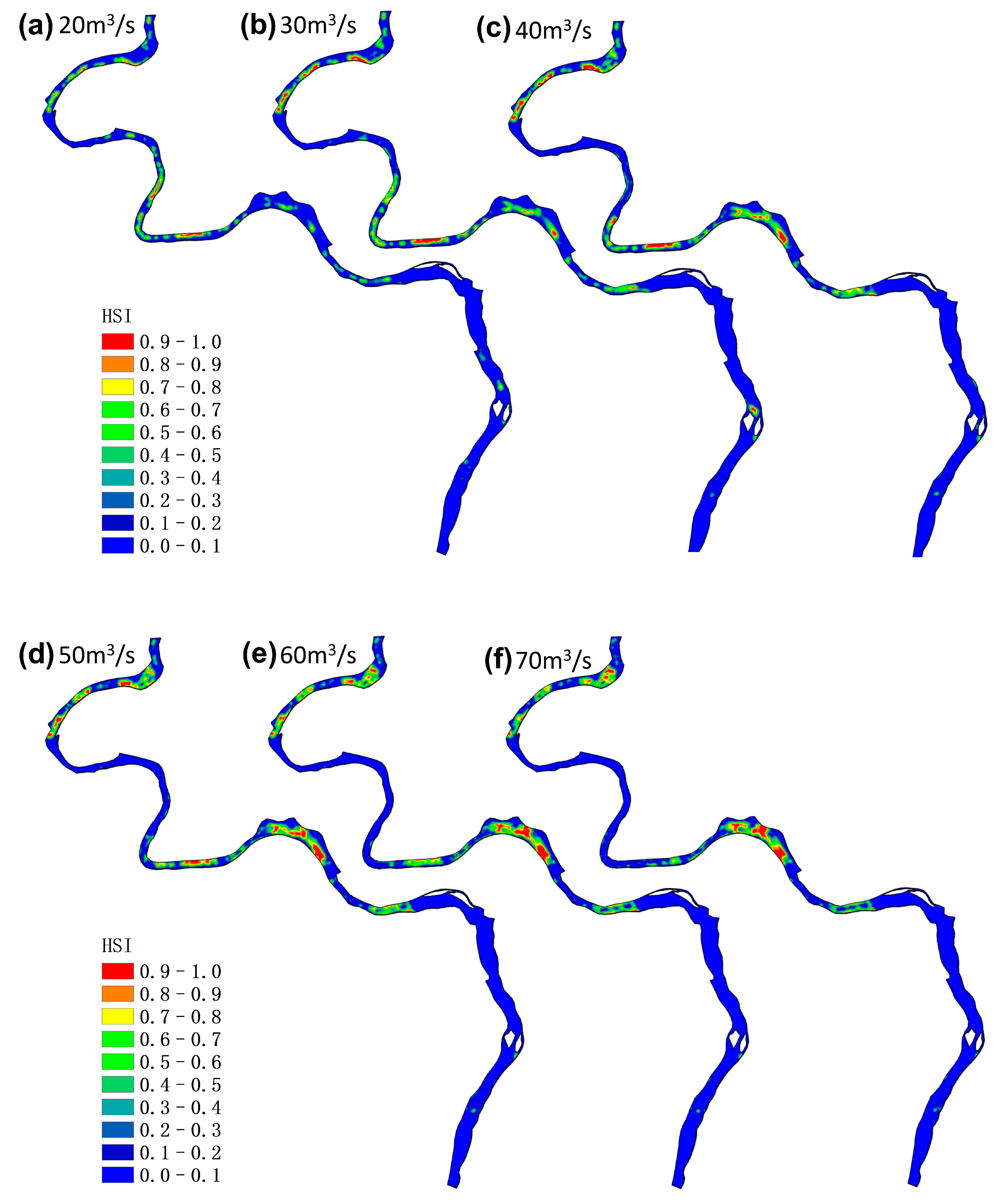
3.2.2. The Change in the Habitat Suitability Index (HSI)

Figure 6 presents the distribution of fish habitat quality in the studied reach using a cloud map of HSI. The majority of high-quality fish habitats are located in the meandering reaches, and the habitat quality appears to increase with an increasing level of discharge. The pie charts in Figure 7 illustrate the proportions of HSI, $D_i$, and $V_i$ in the different reaches under three discharge conditions. In the no-weirs group, at 20 m³/s, HSR had the highest proportion of ideal values and LSR had the lowest. At 40 m³/s, HSR had the highest proportion of ideal values and LSR had the lowest. At 70 m³/s, MSR had the highest proportion of ideal values and HSR had the lowest. In the weir group, at 20 and 40 m³/s, the proportions were the same as those in the no-weirs group. However, at 70 m³/s, HSR had the highest proportion of ideal values and LSR had the lowest. Further comparison between the no-weirs and weir categories within the three sinuosity categories showed that the proportion of ideal values decreased in all categories after the construction of weirs, except for an increase in the HSR category at 70 m³/s. Considering the fact that HSI is calculated using Formula 7, it can be concluded that the habitat quality of this reach is mainly determined by the worse of two factors: water depth or velocity. Therefore, the main factors influencing the habitat quality of different reaches have been identified. At 20 m³/s, the habitat quality of all reaches is mainly determined by velocity; at 40 m³/s, the habitat quality of LSR_w, LSR, MSR_w, and MSR is mainly determined by velocity; and at 70 m³/s, the habitat quality of LSR, MSR, and HSR_w is mainly determined by velocity. At other discharge levels, habitat quality is mainly determined by water depth.

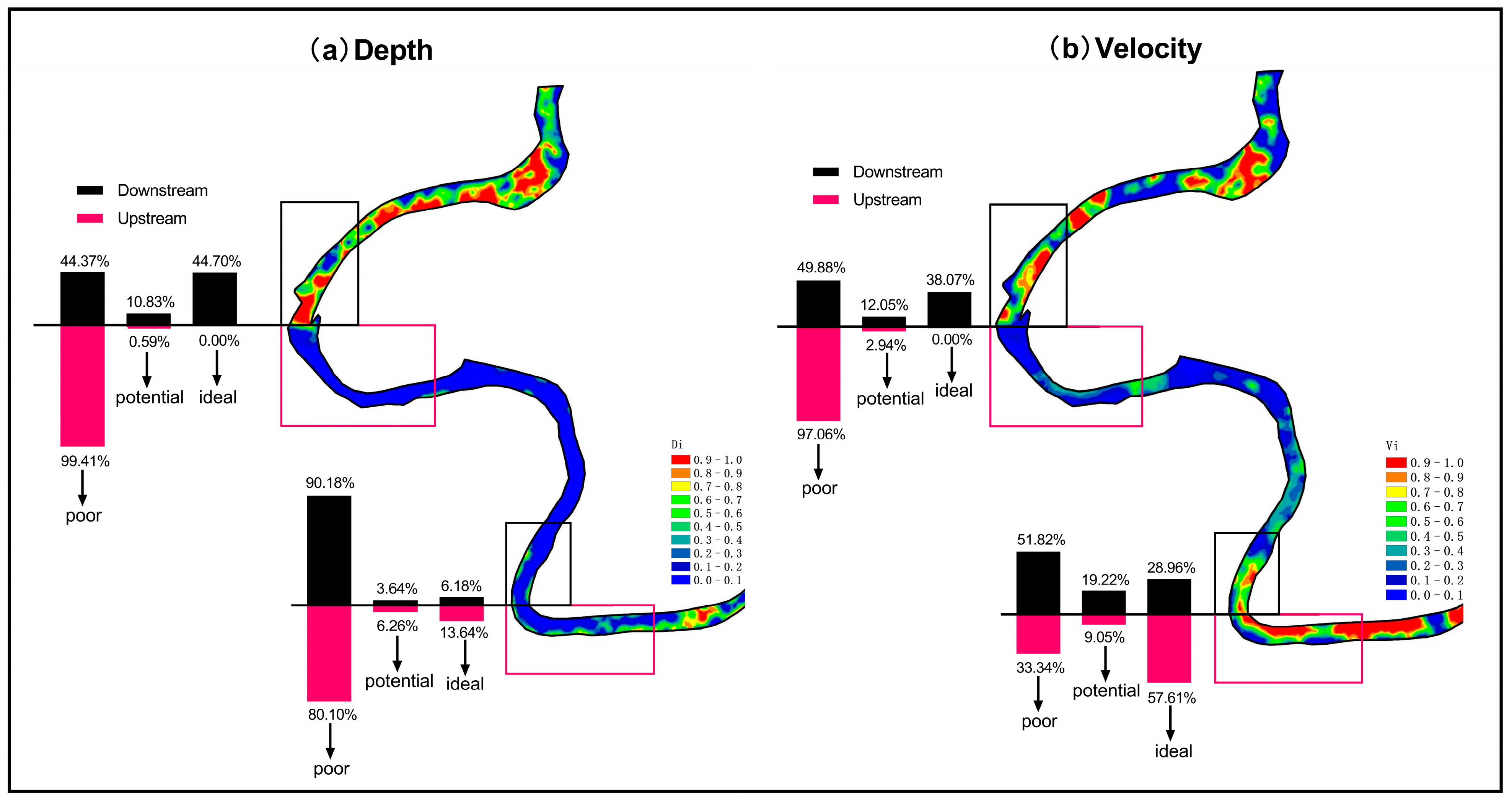
3.2.3. The Specific Distribution of Habitats in the HSR and HSR_w

By referencing the HSI distribution in Figure 6, it can be observed that the distribution of the HSI in the upstream and downstream regions differs for HSR and HSR_w. Therefore, Figure 8 was analyzed to investigate the specific distribution of $D_i$ and $V_i$ under HSR and HSR_w at 70 m³/s. The results showed that in the upstream section of HSR_w, the poor value of $D_i$ (99.41%) was greater than that of $V_i$ (97.06%), indicating the area’s unsuitability for a fish habitat, which is the main factor affecting habitat quality. In the downstream section, velocity is the main factor affecting habitat quality, although both velocity and water depth favorably influence this measure. In the upstream and downstream sections of HSR, the poor value of water depth was greater than that for velocity, indicating that water depth was the main factor affecting habitat quality. However, it is noteworthy that the poor values for both water depth and velocity in the upstream section were lower than those in the downstream section.

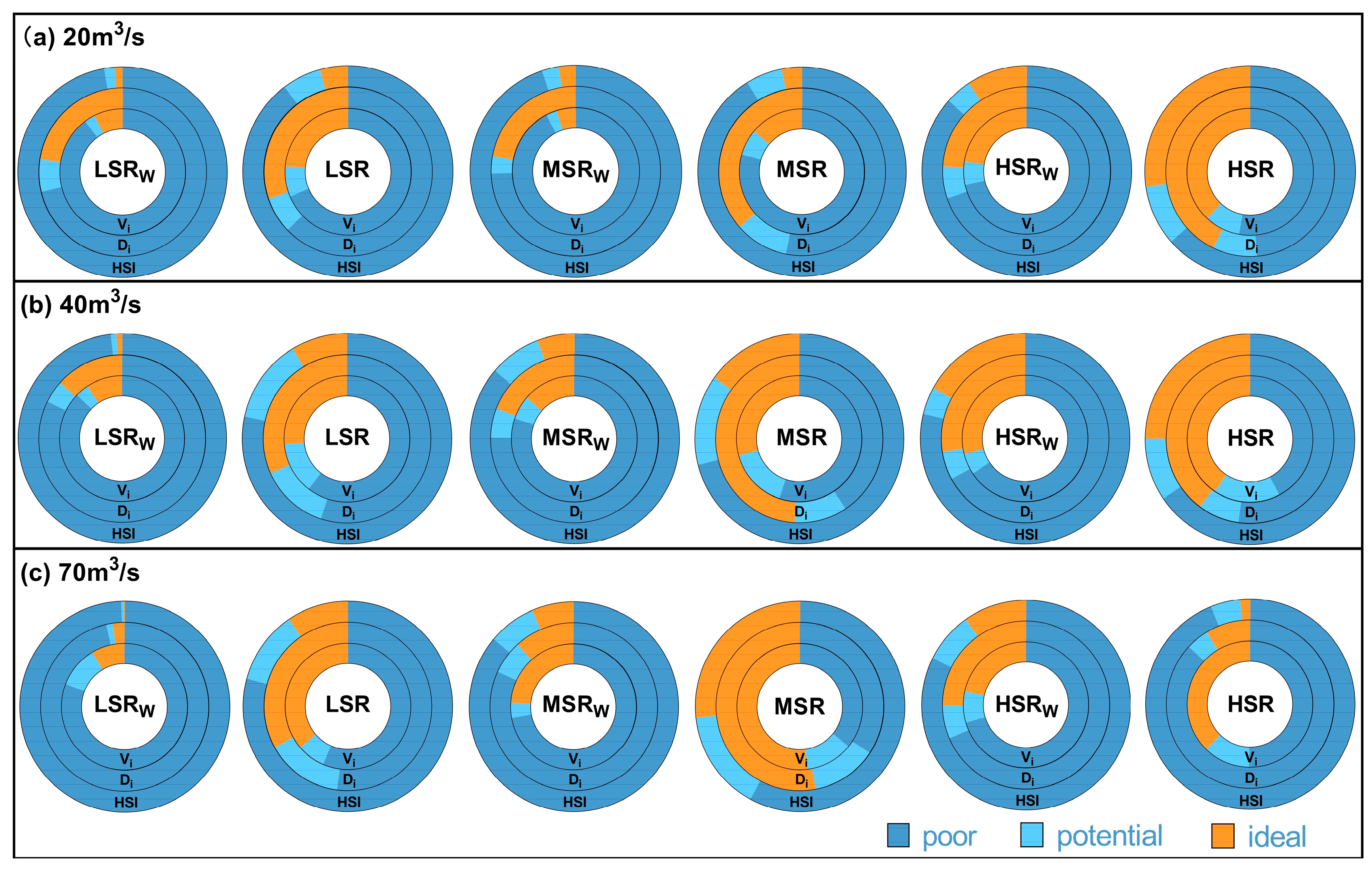
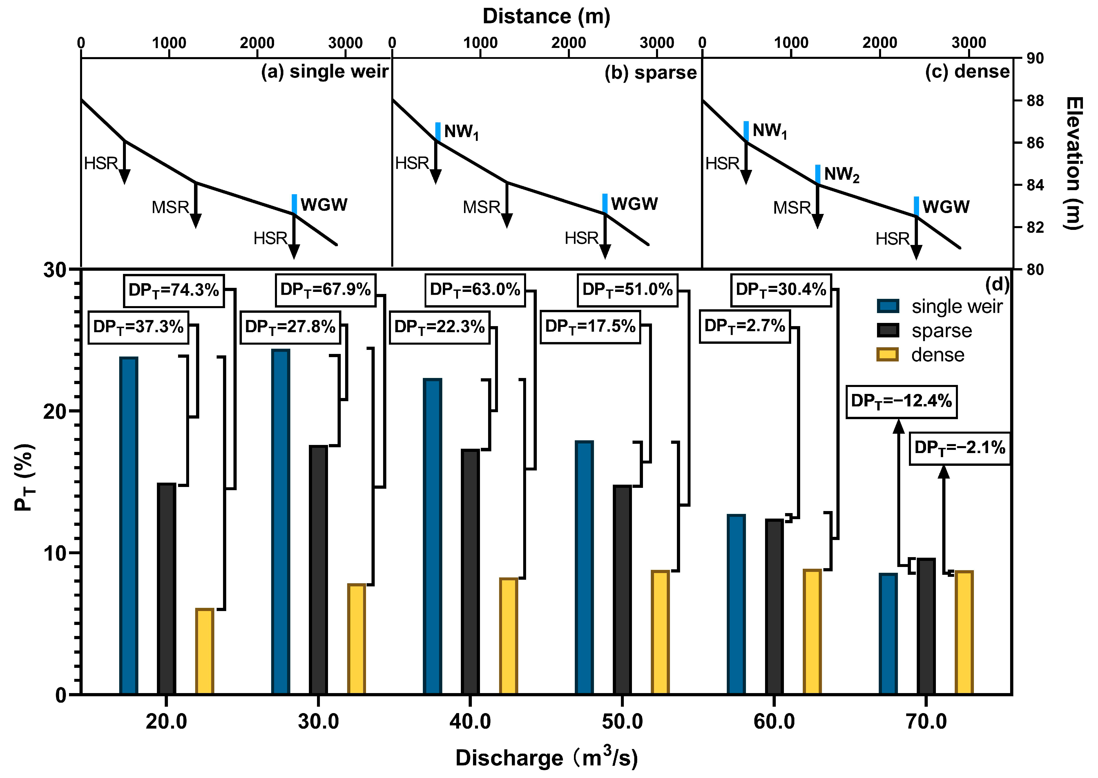
3.3. Change in Fish Habitat Quality in Relation to Different Numbers of Weirs

Figure 9 demonstrates the variation and differences in habitat quality for a particular reach with different numbers of weirs. Figure 9a is the actual situation, indicating a single-weir distribution; Figure 9b is the addition of a weir similar to Wangong Weir, indicating a sparse distribution; and Figure 9c is the addition of two weirs similar to Wangong Weir, indicating a dense distribution. The $P_T$ variation results in Figure 9d illustrate that the $P_T$ of the single-weir distribution is greater than that of the sparse distribution and the dense distribution at 20 m³/s to 60 m³/s. However, at 70 m³/s, the $P_T$ of the single-weir distribution is lower than that of the sparse distribution and the dense distribution. Furthermore, the $P_T$ of the sparse distribution is greater than that of the dense distribution under any discharge conditions. Moreover, the results regarding $D{P}_T$ show that at discharge levels ranging from 20 m³/s to 60 m³/s, the $D{P}_T$ of the sparse distribution decreases from 37.3% to 2.7% and the $D{P}_T$ of the dense distribution decreases from 74.3% to 30.4%, while when the discharge is 70 m³/s, the ${\mathrm{DP}}_{\mathrm{T}}$ of the sparse distribution is −12.4% and the $D{P}_T$ of the dense distribution is −2.1%.

4. Discussion

4.1. Response of Fish Habitat Quality to Sinuosity

In the absence of weirs, habitat quality becomes more stable with changes in discharge as the reach becomes more sinuous, which is a trend that is similar to the findings of Moerke et al. [47], Pedersen et al. [48], and Liu et al. [49]. However, the relationship between sinuosity and habitat quality is not always positive; for HSR, habitat quality is lower than that of MSR when the discharge is between 50 m³/s and 70 m³/s. With the presence of weirs, the habitat quality becomes more concentrated and generally smaller with changes in discharge, while the quality of the habitat in the reach increases with increasing sinuosity. The unsuitability of an HSR’s water depth increases significantly when the discharge increases from 40 m³/s to 70 m³/s, which is the main reason for the decrease in an HSR’s habitat quality. This is mainly because at the same rate of discharge, the water depth in sinuous reaches is significantly greater than that in straight reaches [22]. Moreover, the suitability value is an interval, and when a certain hydraulic condition value exceeds a certain threshold, suitability will decrease. Therefore, under high-discharge conditions, the water depth of highly sinuous reaches far exceeds the suitable water depth, leading to a decrease in habitat quality. To consider the relationship between sinuosity and habitat quality, it is essential to consider the discharge conditions.

4.2. Response of Fish Habitat Quality to Weirs

The results in Figure 5 indicate that there is a decrease in average habitat quality under different discharge conditions in any reach after the construction of weirs. This is consistent with the findings of Musil et al. [50] and Stromberg et al. [51], who reported that the presence of a weir leads to a decrease in habitat quality. It is noteworthy that the habitat quality of HSR_w is greater than that of an HSR at a discharge condition of 70 m³/s, which is different from the previous finding. To further confirm this conclusion, this study added the same weirs to reaches with different sinuosity levels. The results in Figure 9 demonstrate that habitat quality decreases with an increase in the number of weirs for discharge conditions ranging from 20 m³/s to 60 m³/s. However, at a discharge condition of 70 m³/s, a single-weir distribution does not lead to optimal habitat quality, while a sparse distribution (i.e., two weirs) results in the best habitat quality. The reason behind this finding is that NW₁ is located in a high-sinuosity reach while NW₂ is located in a medium-sinuosity reach; thus, at 70 m³/s, NW₁ improves habitat quality and NW₂ degrades it, causing the habitat quality of the sparse weir distribution to be greater than that of the dense weir distribution but less than that of the single-weir distribution. In summary, the impact of weirs on river habitat quality depends on their distribution location and the relevant discharge conditions [16,52].

4.3. Identification of Key Factors Influencing Fish Habitat Quality

At a discharge rate of 70 m³/s, the decline in habitat quality in the HSR is mainly caused by water depth, whereas in the HSR_w, it is caused by velocity. High-sinuosity reaches tend to have lower water depth suitability but higher velocity suitability. The presence of a weir can reduce downstream water depth, greatly improve water depth suitability, and partially improve downstream velocity suitability. However, under the same conditions, upstream velocity suitability decreases significantly, while water depth suitability decreases only slightly. Therefore, it can be inferred that the presence of a weir slightly reduces the suitability of upstream habitats but greatly improves the suitability of downstream habitats by enhancing water depth. There has been extensive research on how weirs alter the hydraulic conditions of upstream and downstream reaches. Weirs are known to decrease downstream water depths and increase downstream velocity [53,54], which we have observed in our own research. Therefore, in high-sinuosity reaches at a discharge of 70 m³/s, the presence of a weir improved the quality of the habitat through improving the downstream water depth. However, under other discharge and sinuosity conditions, the presence of weirs decreased habitat quality. This is because the habitat quality in no-weirs reaches is determined by velocity and not water depth (except for the HSR at a discharge of 70 m³/s). Improving the habitat quality of rivers should not be based on experience, as some recognized measures for improving habitat quality may not be effective under certain conditions [55] or may have different effects depending on the discharge and layout conditions [56,57]. These findings are similar to our research conclusion; that is, the impact of hydraulic engineering on habitat quality will vary according to flow and layout conditions. Therefore, it is necessary to have a clear understanding of the effects of hydraulic engineering on reaches corresponding to different layouts and under different discharge conditions to guide designs and achieve the desired results.

However, in this study, the impact of the specific location of a weir on habitat quality was not fully considered; only the effect of the general position of a weir on a meandering reach was taken into account. Some studies have shown that a reach can be divided into two different sections: a curved segment and a transitional straight segment between two curves. These two segments have very different impacts on habitat quality [49]. Additionally, we did not fully consider the influences on migratory fish, as weirs may hinder fish migration; however, regarding overflow weirs, this study shows that under long-term high-discharge submergence conditions, the presence of a weir may cause fish to move upstream [58]. Currently, there are numerous hydrodynamic models available, and in this study, we employed a two-dimensional (2D) hydrodynamic model for simulation. Additionally, within the context of habitat modeling, some studies have utilized one-dimensional (1D) hydrodynamic models [12]. The key distinction between the two models is the enhanced precision of 2D models under more complex conditions [59]. Therefore, for this study, which involves intricate mountainous terrain and multiple hydraulic structures in rivers, the utilization of a 2D hydrodynamic model was deemed more appropriate and may even allow for the development of a three-dimensional (3D) model. Nevertheless, it is important to acknowledge that compared to 1D models, 2D models require more effort and time dedicated to the calibration and validation of river channels [59]. Hence, in urban rivers or rivers with fewer hydraulic structures, the adoption of a 1D hydrodynamic model may be a more suitable choice. Overall, the consideration of the ecological effects of hydraulic structures on fish is an ongoing process that requires continuous refinement.

5. Conclusions

This study demonstrates that the impact of weirs on the habitat quality of rivers is closely related to the relevant discharge conditions and layout. This is because the key hydraulic factors that influence the suitability of a habitat for a reach change under different conditions. Therefore, by analyzing the suitability of water depth or velocity, we can identify the key hydraulic factors that affect the suitability of a habitat for a given reach and develop corresponding habitat quality improvement plans. In this study, it was found that the habitat quality of highly meandering reaches with a 70 m³/s discharge rate was primarily determined by water depth, with the downstream water depth being unsuitable for fish survival. Therefore, improving downstream water depth distribution using weirs can enhance the habitat quality of highly meandering river segments. Under other conditions, if velocity is the key factor, measures to improve flow velocity suitability can be taken. This study provides recommendations for protecting the habitat quality of fish in small and medium-sized mountainous rivers and for determining the locations of weirs. Although these conclusions may not apply to larger rivers and other hydraulic structures, they still provide a research direction for considering the response of fish habitat quality to hydraulic structures under different discharge conditions and layouts.

References

1. Stadtmann, S.; Seddon, P.J. Release site selection: Reintroductions and the habitat concept. Oryx 2020, 54, 687–695. [Google Scholar] [CrossRef]
2. Yang, Z.; Hu, P.; Wang, J.; Zhao, Y.; Zhang, W. Ecological flow process acknowledging different spawning patterns in the Songhua River. Ecol. Eng. 2019, 132, 56–64. [Google Scholar] [CrossRef]
3. Poff, N.L.; Hart, D.D. How dams vary and why it matters for the emerging science of dam removal. Bioscience 2002, 52, 659–668. [Google Scholar] [CrossRef]
4. Zaidel, P.A.; Roy, A.H.; Houle, K.M.; Lambert, B.; Letcher, B.H.; Nislow, K.H.; Smith, C. Impacts of small dams on stream temperature. Ecol. Indic. 2021, 120, 106878. [Google Scholar] [CrossRef]
5. Mueller, M.; Pander, J.; Geist, J. The effects of weirs on structural stream habitat and biological communities. J. Appl. Ecol. 2011, 48, 1450–1461. [Google Scholar] [CrossRef]
6. Pander, J.; Geist, J. Ecological indicators for stream restoration success. Ecol. Indic. 2013, 30, 106–118. [Google Scholar] [CrossRef]
7. Meixler, M.S.; Bain, M.B.; Walter, M.T. Predicting barrier passage and habitat suitability for migratory fish species. Ecol. Model. 2009, 220, 2782–2791. [Google Scholar] [CrossRef]
8. Jager, H.I.; Chandler, J.A.; Lepla, K.B.; Van Winkle, W. A theoretical study of river fragmentation by dams and its effects on white sturgeon populations. Environ. Biol. Fishes 2001, 60, 347–361. [Google Scholar] [CrossRef]
9. Birnie-Gauvin, K.; Candee, M.M.; Baktoft, H.; Larsen, M.H.; Koed, A.; Aarestrup, K. River connectivity reestablished: Effects and implications of six weir removals on brown trout smolt migration. River Res. Appl. 2018, 34, 548–554. [Google Scholar] [CrossRef]
10. Mouton, A.M.; Schneider, M.; Depestele, J.; Goethals, P.L.M.; De Pauw, N. Fish habitat modelling as a tool for river management. Ecol. Eng. 2007, 29, 305–315. [Google Scholar] [CrossRef]
11. Im, D.; Kang, H.; Kim, K.-H.; Choi, S.-U. Changes of river morphology and physical fish habitat following weir removal. Ecol. Eng. 2011, 37, 883–892. [Google Scholar] [CrossRef]
12. Tang, L.; Mo, K.; Zhang, J.; Wang, J.; Chen, Q.; He, S.; Zhu, C.; Lin, Y. Removing tributary low-head dams can compensate for fish habitat losses in dammed rivers. J. Hydrol. 2021, 598, 126204. [Google Scholar] [CrossRef]
13. Al-Zankana, A.F.A.; Matheson, T.; Harper, D.M. How strong is the evidence—Based on macroinvertebrate community responses—That river restoration works? Ecohydrol. Hydrobiol. 2020, 20, 196–214. [Google Scholar] [CrossRef]
14. Nagayama, S.; Ishiyama, N.; Seno, T.; Kawai, H.; Kawaguchi, Y.; Nakano, D.; Nakamura, F. Time Series Changes in Fish Assemblages and Habitat Structures Caused by Partial Check Dam Removal. Water 2020, 12, 3357. [Google Scholar] [CrossRef]
15. Foley, M.M.; Bellmore, J.R.; O’Connor, J.E.; Duda, J.J.; East, A.E.; Grant, G.E.; Anderson, C.W.; Bountry, J.A.; Collins, M.J.; Connolly, P.J.; et al. Dam removal: Listening in. Water Resour. Res. 2017, 53, 5229–5246. [Google Scholar] [CrossRef]
16. Gore, J.A.; Hamilton, S.W. Comparison of flow-related habitat evaluations downstream of low-head weirs on small and large fluvial ecosystems. Regul. Rivers-Res. Manag. 1996, 12, 459–469. [Google Scholar] [CrossRef]
17. Zhu, Z.-X.; Li, Y.; Li, K.-F.; Cheng, B.-X.; Yang, S.-R.; Liu, Q.-Y.; Qing, J.; Zhang, B.-C.; Yan, X.; Liang, R.-F. Study of quality maintenance of fish habitats in small- and medium-sized mountain rivers with low flow rate. Ecol. Eng. 2020, 147, 105780. [Google Scholar] [CrossRef]
18. Crowder, D.W.; Diplas, P. Using two-dimensional hydrodynamic models at scales of ecological importance. J. Hydrol. 2000, 230, 172–191. [Google Scholar] [CrossRef]
19. Roni, P.; Bennett, T.; Morley, S.; Pess, G.R.; Hanson, K.; Van Slyke, D.; Olmstead, P. Rehabilitation of bedrock stream channels: The effects of boulder weir placement on aquatic habitat and biota. River Res. Appl. 2006, 22, 967–980. [Google Scholar] [CrossRef]
20. Lee, J.H.; Kil, J.T.; Jeong, S. Evaluation of physical fish habitat quality enhancement designs in urban streams using a 2D hydrodynamic model. Ecol. Eng. 2010, 36, 1251–1259. [Google Scholar] [CrossRef]
21. Flotemersch, J.E.; North, S.; Blocksom, K.A. Evaluation of an alternate method for sampling benthic macroinvertebrates in low-gradient streams sampled as part of the National Rivers and Streams Assessment. Environ. Monit. Assess. 2014, 186, 949–959. [Google Scholar] [CrossRef] [PubMed]
22. Yu, Z.; Zhang, J.; Wang, H.; Zhao, J.; Dong, Z.; Peng, W.; Zhao, X. Quantitative analysis of ecological suitability and stability of meandering rivers. Front. Biosci.-Landmark 2022, 27, 42. [Google Scholar] [CrossRef] [PubMed]
23. Zhou, T.; Endreny, T. The Straightening of a River Meander Leads to Extensive Losses in Flow Complexity and Ecosystem Services. Water 2020, 12, 1680. [Google Scholar] [CrossRef]
24. Lorenz, A.W.; Jaehnig, S.C.; Hering, D. Re-Meandering German Lowland Streams: Qualitative and Quantitative Effects of Restoration Measures on Hydromorphology and Macroinvertebrates. Environ. Manag. 2009, 44, 745–754. [Google Scholar] [CrossRef] [PubMed]
25. Nakano, D.; Nakamura, F. The significance of meandering channel morphology on the diversity and abundance of macroinvertebrates in a lowland river in Japan. Aquat. Conserv.-Mar. Freshw. Ecosyst. 2008, 18, 780–798. [Google Scholar] [CrossRef]
26. Leopold, L.B.; Wolman, M.G.; Miller, J.P.; Wohl, E. Fluvial Processes in Geomorphology; Dover Publications: Mineola, NY, USA, 2020. [Google Scholar]
27. Rust, B.R. A classification of alluvial channel systems. In Fluvial Sedimentology; Miall, A.D., Ed.; Datapages, Inc.: Tulsa, OK, USA, 1978. [Google Scholar]
28. Hauer, C.; Unfer, G.; Holzmann, H.; Schmutz, S.; Habersack, H. The impact of discharge change on physical instream habitats and its response to river morphology. Clim. Change 2013, 116, 827–850. [Google Scholar] [CrossRef]
29. Garcia, X.F.; Schnauder, I.; Pusch, M.T. Complex hydromorphology of meanders can support benthic invertebrate diversity in rivers. Hydrobiologia 2012, 685, 49–68. [Google Scholar] [CrossRef]
30. Hung, H.-J.; Lo, W.-C.; Chen, C.-N.; Tsai, C.-H. Fish’ habitat area and habitat transition in a river under ordinary and flood flow. Ecol. Eng. 2022, 179, 106606. [Google Scholar] [CrossRef]
31. Gauld, N.R.; Campbell, R.N.B.; Lucas, M.C. Reduced flow impacts salmonid smolt emigration in a river with low-head weirs. Sci. Total Environ. 2013, 458, 435–443. [Google Scholar] [CrossRef]
32. Melcher, A.H.; Schmutz, S. The importance of structural features for spawning habitat of nase Chondrostoma nasus (L.) and barbel Barbus barbus (L.) in a pre-Alpine river. River Syst. 2010, 19, 33–42. [Google Scholar] [CrossRef]
33. Ran, Y.; Liu, Y.; Wu, S.; Li, W.; Zhu, K.; Ji, Y.; Mir, Y.; Ma, M.; Huang, P. A higher river sinuosity increased riparian soil structural stability on the downstream of a dammed river. Sci. Total Environ. 2022, 802, 149886. [Google Scholar] [CrossRef]
34. Shan, C.; Guo, H.; Dong, Z.; Liu, L.; Lu, D.; Hu, J.; Feng, Y. Study on the river habitat quality in Luanhe based on the eco-hydrodynamic model. Ecol. Indic. 2022, 142, 109262. [Google Scholar] [CrossRef]
35. Zhang, X.; Duan, B.; He, S.; Lu, Y. Simulation study on the impact of ecological water replenishment on reservoir water environment based on Mike21—Taking Baiguishan reservoir as an example. Ecol. Indic. 2022, 138, 108802. [Google Scholar] [CrossRef]
36. Vozinaki, A.-E.K.; Morianou, G.G.; Alexakis, D.D.; Tsanis, I.K. Comparing 1D and combined 1D/2D hydraulic simulations using high-resolution topographic data: A case study of the Koiliaris basin, Greece. Hydrol. Sci. J. 2017, 62, 642–656. [Google Scholar] [CrossRef]
37. Nash, J.E.; Sutcliffe, J.V. River flow forecasting through conceptual models part I—A discussion of principles. J. Hydrol. 1970, 10, 282–290. [Google Scholar] [CrossRef]
38. Moriasi, D.; Arnold, J.; Van Liew, M.; Bingner, R.; Harmel, R.D.; Veith, T. Model Evaluation Guidelines for Systematic Quantification of Accuracy in Watershed Simulations. Trans. ASABE 2007, 50, 885–900. [Google Scholar] [CrossRef]
39. Urich, D.L.; Graham, J.P. Applying habitat evaluation procedures (HEP) to wildlife area planning in Missouri. Wildl. Soc. Bull. (1973–2006) 1983, 11, 215–222. [Google Scholar]
40. Wang, F. Experimental and Numerical Analysis of River Lake System and Non-Traditional Water Usage in a New Eco-City. Ph.D. Thesis, Cardiff University, Cardiff, UK, 2013. [Google Scholar]
41. Yao, W.; Minh Duc, B.; Rutschmann, P. Development of eco-hydraulic model for assessing fish habitat and population status in freshwater ecosystems. Ecohydrology 2018, 11, e1961. [Google Scholar] [CrossRef]
42. Jowett, I.G.; Davey, A.J.H. A comparison of composite habitat suitability indices and generalized additive models of invertebrate abundance and fish presence-habitat availability. Trans. Am. Fish. Soc. 2007, 136, 428–444. [Google Scholar] [CrossRef]
43. Wang, F.; Lin, B. Modelling habitat suitability for fish in the fluvial and lacustrine regions of a new Eco-City. Ecol. Model. 2013, 267, 115–126. [Google Scholar] [CrossRef]
44. Bovee, K.D. A Guide to Stream Habitat Analysis Using the Instream Flow Incremental Methodology; IFIP No. 12; FWS/0 BS-82/26; Alaska Reources Library & Information Setvices: Anchorage, AK, USA, 1982. [Google Scholar]
45. Reglero, P.; Ortega, A.; Blanco, E.; Fiksen, O.; Viguri, F.J.; de la Gandara, F.; Seoka, M.; Folkvord, A. Size-related differences in growth and survival in piscivorous fish larvae fed different prey types. Aquaculture 2014, 433, 94–101. [Google Scholar] [CrossRef]
46. Yi, Y.; Cheng, X.; Yang, Z.; Wieprecht, S.; Zhang, S.; Wu, Y. Evaluating the ecological influence of hydraulic projects: A review of aquatic habitat suitability models. Renew. Sustain. Energy Rev. 2017, 68, 748–762. [Google Scholar] [CrossRef]
47. Moerke, A.H.; Gerard, K.J.; Latimore, J.A.; Hellenthal, R.A.; Lamberti, G.A. Restoration of an Indiana, USA, stream: Bridging the gap between basic and applied lotic ecology. J. N. Am. Benthol. Soc. 2004, 23, 647–660. [Google Scholar] [CrossRef]
48. Pedersen, M.L.; Friberg, N.; Skriver, J.; Baattrup-Pedersen, A.; Larsen, S.E. Restoration of Skjern River and its valley—Short-term effects on river habitats, macrophytes and macroinvertebrates. Ecol. Eng. 2007, 30, 145–156. [Google Scholar] [CrossRef]
49. Liu, J.; Zhang, X.; Xu, Z.; Wang, J.; Ma, B.; Xue, R.; Li, Q. Evaluation of the impact of urban river bends on the enhancement of aquatic habitats using a two-dimensional habitat suitability model. Ecol. Inform. 2021, 65, 101428. [Google Scholar] [CrossRef]
50. Musil, J.; Horky, P.; Slavik, O.; Zboril, A.; Horka, P. The response of the young of the year fish to river obstacles: Functional and numerical linkages between dams, weirs, fish habitat guilds and biotic integrity across large spatial scale. Ecol. Indic. 2012, 23, 634–640. [Google Scholar] [CrossRef]
51. Stromberg, J.C.; Beauchamp, V.B.; Dixon, M.D.; Lite, S.J.; Paradzick, C. Importance of low-flow and high-flow characteristics to restoration of riparian vegetation along rivers in and south-western United States. Freshw. Biol. 2007, 52, 651–679. [Google Scholar] [CrossRef]
52. Radinger, J.; Hoelker, F.; Horky, P.; Slavik, O.; Wolter, C. Improved river continuity facilitates fishes’ abilities to track future environmental changes. J. Environ. Manag. 2018, 208, 169–179. [Google Scholar] [CrossRef]
53. Bagheri, S.; Kabiri-Samani, A. Simulation of free surface flow over the streamlined weirs. Flow Meas. Instrum. 2020, 71, 101680. [Google Scholar] [CrossRef]
54. Soydan Oksal, N.G.; Akoz, M.S.; Simsek, O. Experimental analysis of flow characteristics over hydrofoil weirs. Flow Meas. Instrum. 2021, 79, 101867. [Google Scholar] [CrossRef]
55. De Jalon, D.G.; Gortazar, J. Evaluation of instream habitat enhancement options using fish habitat simulations: Case-studies in the river Pas (Spain). Aquat. Ecol. 2007, 41, 461–474. [Google Scholar] [CrossRef]
56. Ma, B.; Dong, F.; Peng, W.Q.; Liu, X.B.; Huang, A.P.; Zhang, X.H.; Liu, J.Z. Evaluation of impact of spur dike designs on enhancement of aquatic habitats in urban streams using 2D habitat numerical simulations. Glob. Ecol. Conserv. 2020, 24, e01288. [Google Scholar] [CrossRef]
57. Yang, X.; Zhang, S.; Li, W.; Tang, C.; Zhang, J.; Schwindt, S.; Wieprecht, S.; Wang, T. Impact of the construction of a dam and spur dikes on the hydraulic habitat of Megalobrama terminalis spawning sites: A case study in the Beijiang River (China). Ecol. Indic. 2022, 143, 109361. [Google Scholar] [CrossRef]
58. Keller, R.J.; Peterken, C.J.; Berghuis, A.P. Design and assessment of weirs for fish passage under drowned conditions. Ecol. Eng. 2012, 48, 61–69. [Google Scholar] [CrossRef]
59. Jowett, I.G.; Duncan, M.J. Effectiveness of 1D and 2D hydraulic models for instream habitat analysis in a braided river. Ecol. Eng. 2012, 48, 92–100. [Google Scholar] [CrossRef]
Figure 1. Location of the study area, weirs, and the hydrological station.
Sustainability 15 08698 g001
Figure 2. Schematic diagram of river sinuosity calculation.
Sustainability 15 08698 g002
Figure 3. Habitat suitability index.
Sustainability 15 08698 g003
Figure 4. Locations of morphologically different reaches.
Sustainability 15 08698 g004
Figure 5. (a) The P T relative to six discharge conditions in the reaches with different sinuosity values. (b) The change in P T with sinuosity for six discharges in no-weirs category. (c) The change in P T with sinuosity for six discharges in weir category (The red line represents an initial increase followed by a subsequent decrease, while the blue line indicates a continuous upward trend.).
Sustainability 15 08698 g005
Figure 6. Cloud map of the habitat suitability index’s (HSI) spatial distribution.
Sustainability 15 08698 g006
Figure 7. Pie charts of the habitat suitability index (HSI), V i , and D i .
Sustainability 15 08698 g007
Figure 8. (a) Cloud map of the specific distribution of D i under HSR and HSRw at 70 m3/s. (b) Cloud map of the specific distribution of V i under HSR and HSRw at 70 m3/s.
Sustainability 15 08698 g008
Figure 9. (a) The distribution of a single weir (WGW—Wangong Weir); (b) the distribution of sparse weirs (NW1—a new weir, which is similar to Wangong Weir); (c) the distribution of dense weirs (NW1 and NW2 denote two new weirs, which are similar to Wangong Weir); (d) the percentage of WUA with respect to the total area ( P T ) variation for three different quantities of weirs ( D P T represents the difference in P T between the different numbers of weirs).
Sustainability 15 08698 g009