Displacement Field Calculation of Large-Scale Structures Using Computer Vision with Physical Constraints: An Experimental Study

Abstract

In recent years, computer vision-based structural displacement acquisition technique has received wide attention and research due to the advantages of easy deployment, low-cost, and non-contact. However, the displacement field acquisition of large-scale structures is a challenging topic as a result of the contradiction of camera field-of-view and resolution. This paper presents a large-scale structural displacement field calculation framework with integrated computer vision and physical constraints using only one camera. First, the full-field image of the large-scale structure is obtained by processing the multi-view image using image stitching technique; second, the full-field image is meshed and the node displacements are calculated using an improved template matching method; and finally, the non-node displacements are described using shape functions considering physical constraints. The developed framework was validated using a scaled bridge model and evaluated by the proposed evaluation index for displacement field calculation accuracy. This paper can provide an effective way to obtain displacement fields of large-scale structures efficiently and cost-effectively.

1. Introduction

Displacement information, especially structural displacement field information, is essential for accurate service condition assessment of large-scale engineering structures. The analysis of structural displacements allows for the sensing of local or global damage to the structure, and is an important basic response type for structural modal identification, damage identification, and safety assessment [1,2,3,4,5,6,7,8]. Therefore, many types of displacement sensing devices have been used in structural health monitoring systems or structural inspection process [9,10,11,12,13,14], which can be divided into contact-based and non-contact-based.

Contact-based sensing methods include optic fiber sensors, piezoelectric sensors, strain gauge sensors, linear variable differential transformer (LVDT) and GPS, of which the latter two are the most commonly used [15,16,17,18,19,20]. The limitation of these two methods is the need for complex installations close to the structure. LVDT measures the relative displacement of a structure to a stationary point, meaning that a stationary point close to the structure must be set free from any vibration, which is often difficult to find in practice. GPS calculates the displacement by measuring the coordinates of the equipment installed on the structure. In addition to being expensive, the measurement accuracy is very limited, usually ±1.5 cm in the horizontal direction and ±2 cm in the vertical direction. The non-contact-based displacement sensor has the advantage of remote measurement without the need for complex installation on the structure. As a widely used non-contact sensor, laser displacement sensor needs a stationary point similar to LVDT, but the measurement distance cannot be considerably far due to the limitation of laser intensity.

Non-contact-based sensing methods include X-ray tomography, digital image correlation (DIC), and computer vision-based approaches. The first two are the primary choices for displacement or strain measurement of small-scale structures, such as laboratory specimens, but the measurement equipment is expensive and there are limitations, such as limited measurement range [21]. Vision-based displacement sensors have received extensive attention from researchers due to their low-cost, long measurement distance, multiple measurement points, and high measurement accuracy [22,23]. Vision-based structural displacement measurement calculates the displacement of a structure by comparing the position changes in the same pixels of different frames of the time-series images (video) of the structure remotely captured by cameras. Template matching and its variants are often used to find the location of the same pixel in different frames, namely, tracking. To reduce the difficulty of tracking, initial research has been carried out to increase the recognizability of the appearance by matching artificial markers or targets installed at the location of the structure. With the improvement of the complexity and robustness of algorithms, satisfactory accuracy can be obtained by directly using the natural texture of the structure for tracking. Feng and Feng [24] proposed a multi-point simultaneous extraction method of structural displacement based on two improved template matching methods (using only one camera). Aoyama et al. [25] developed a multiple vibration distribution synthesis method to perform modal analysis on large-scale structures by using a multithread active vision system and a galvanometer mirror to perform quasi-real-time observation of multiple points of the structure. Luo et al. [26] proposed a set of image processing algorithms after analyzing the problems in practical outdoor applications, including the use of gradient-based template matching method, sub-pixel method, and camera vibration elimination method. Due to the limited field-of-view of a single camera, Lydon et al. [27] developed multi-point displacement measurement system for large-scale structures using multiple time-synchronized wireless cameras and successfully applied it to actual bridge displacement measurements. Xu et al. [28] presented a multi-point displacement extraction method for real cable-stayed pedestrian bridges using consumer-grade cameras and computer vision algorithms. To solve the problem that the traditional image methods are not robust enough to the change in ambient light intensity, Song et al. [29] proposed the use of fully convolutional network and conditional random field to segment the structural part from the image in order to extract the multi-point displacement combined with the digital image correlation method. These methods are aimed at extracting the displacement of one or several positions of the structure to be measured, namely, local displacement measurement.

Compared with local displacement, full-field displacement information of structures can provide more abundant structural state information for finite element model updating, material performance parameter identification, and structural condition assessment [30]. By comparing the displacement field of the key surface of the structure at different service times, the global performance change in the structure can be reflected. Thanks to its distributed sensing characteristics, it can also reflect the local performance change in the structure, to realize the global and local structural performance evaluation. In addition, the visual sensor has the advantage of large-scale dense sensing, and thus it is more meaningful to conduct vision-based structural full-field displacement measurement. Compared with previous tracking methods, such as digital image correlation or template matching, the phase-based method fits the full-field information acquisition and can obtain subpixel displacement measurement accuracy. Shang and Shen [31] proposed the use of the phase-based optical flow method to obtain the full-field vibration map of the structure and use the motion magnification technology to identify the modal parameters. Yang et al. [32,33] used the physics-guided unsupervised machine learning vision method to identify the full-field vibration modes of stay cables, and for the vibration structure with large rigid body displacement, a vision-based simultaneous identification method of rigid body displacement and structural vibration was also proposed, which was verified on the laboratory model. Narazaki et al. [34,35] developed a vision-based algorithm for measuring the dense three-dimensional displacement field of structures, and optimized the algorithm parameters using a laboratory truss model. Bhowmick and Nagarajaiah [36,37,38] proposed the use of the continuous edges of the structure in the image as texture features and the combination of the optical flow method to extract the full-field displacement of the structure, and verified it on the three-layer steel frame model in the laboratory. To further simplify the measurement process of structural full-field displacement, Luan et al. [39] developed a deep learning extraction framework for structural full-field displacement based on convolutional neural networks, which realized real-time measurement of full-field subpixel displacement and verified it on a laboratory model. These studies have greatly promoted the development of structural full-field displacement measurement. However, since most of the work has been verified by small-scale laboratory models, a main problem in actual large-scale structural full-field displacement measurement is not involved: Full-field structure image acquisition.

In vision-based structural displacement measurement, each pixel can be regarded as a sensor, and the actual distance it represents is the resolution of the measurement system. Although the accuracy can be further improved by means of subpixel technology, it can only be amplified by an extremely limited multiple. Therefore, obtaining a full-field image of the structure with sufficient resolution is the basis of full-field displacement measurement. Due to the small size of the laboratory model, the field-of-view of a camera can cover the entire structure with good resolution. However, actual civil structures tend to be large; therefore, if only one camera will be used to shoot all the structure, this will result in an extremely low resolution, and to maintain the resolution, the camera’s field-of-view is quite small to cover the whole structure.

To solve the image acquisition and processing problem in full-field displacement measurement of large-scale structures, this paper presents a novel calculation framework of large-scale structural displacement field. To alleviate the contradiction between camera field-of-view and resolution, image stitching technology based on multi-view images is proposed to generate large-scale structure full-field images. To improve the efficiency of displacement extraction and consider the physical rules, the node and non-node displacement extraction technology based on meshing and structural shape function is developed.

The contribution of this paper is that the plane displacement field of large-scale structure can be obtained by using only a single camera and an automatic rotating platform, which greatly simplifies the process and cost of displacement field acquisition. Specifically, this paper first proposes a sensing system for the plane displacement field of large structures, which can automatically image and stitch large structures through a rotating platform. Second, this paper proposes a node and non-node meshing method for large-scale structural planes, and develops a displacement calculation method for nodes and non-nodes, respectively. The non-node displacement calculation considers physical constraints and accelerates the displacement calculation process.

The remainder of this paper is organized as follows. Section 2 describes the details of the proposed structural displacement field calculation framework. Section 3 illustrates the verification results and discusses the key parameters of the presented method. Finally, Section 4 concludes the study.

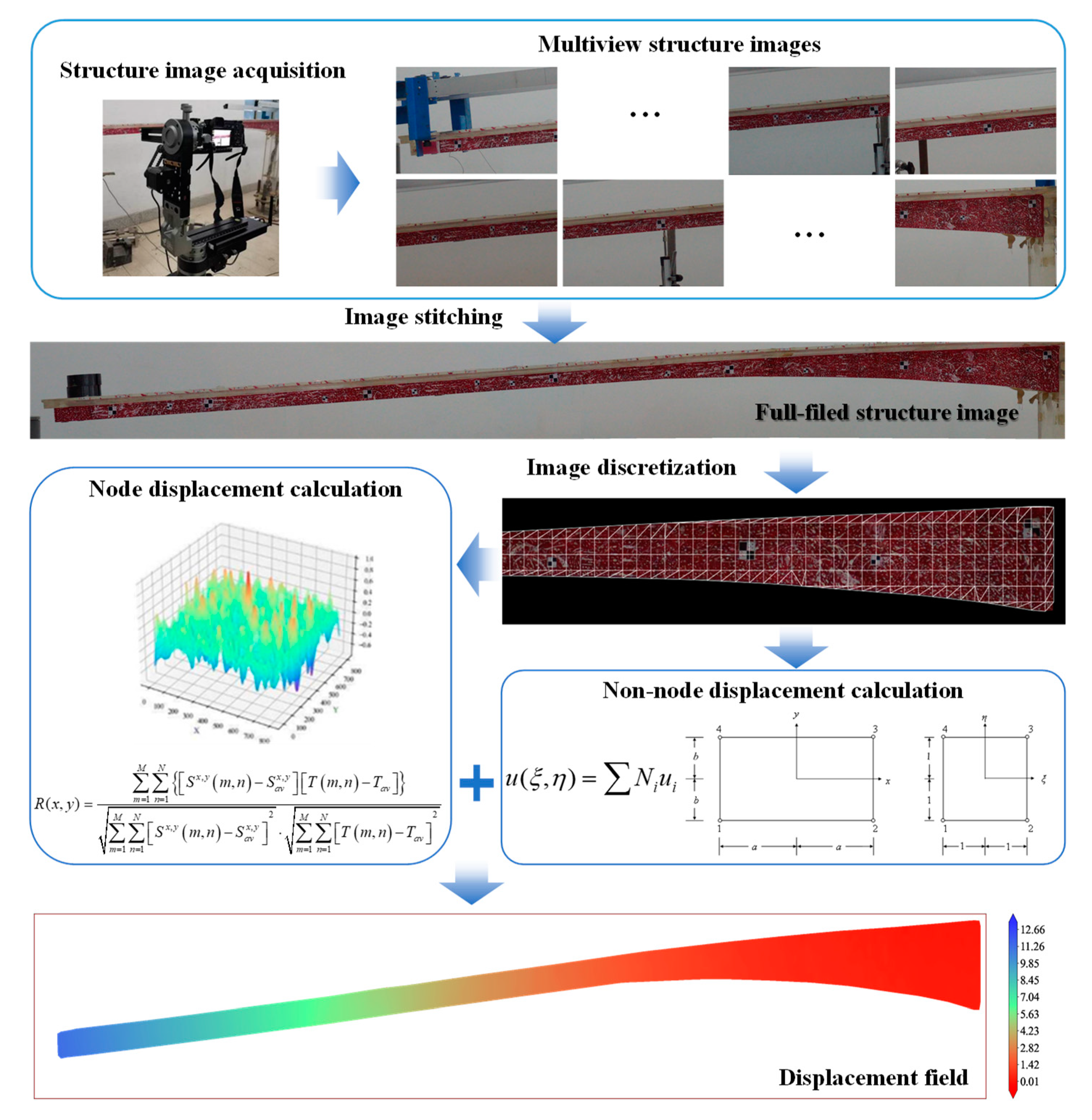
2. Structural Displacement Field Calculation Framework

The proposed calculation framework of structural displacement field is shown in Figure 1. The proposed method can perform two-dimensional fast imaging and fast calculation of displacement field for key planes of large-scale structures. First, a camera set on the automatic rotation device is used to shoot the large-scale structure to obtain a multi-view structure image, it should be noted that the rotating plane is horizontal, namely, the optical axis of the camera is ensured to be horizontal. Second, the full-field structure image is generated by using image stitching technology. Finally, the full-field image is discretized and meshed, the displacement at the node is calculated by the improved template matching method, and the displacement at the non-node is calculated by the shape function considering the physical rules, to obtain the displacement field of the large-scale structure.

2.1. Large-Scale Structure Full-Field Image Generation Using Image Stitching

To obtain high-resolution full-field images of large-scale structures, this paper proposes a full-field image generation method that rotates and moves a single camera to capture multiple partial structure images and stitch them together. The proposed generation method is divided into three steps: (1) Image preprocessing (used to solve the problem of inconsistent depth of field); (2) image registration (used to align and stitch multi-view images); (3) structure foreground segmentation (used to extract the structure in the full-field image).

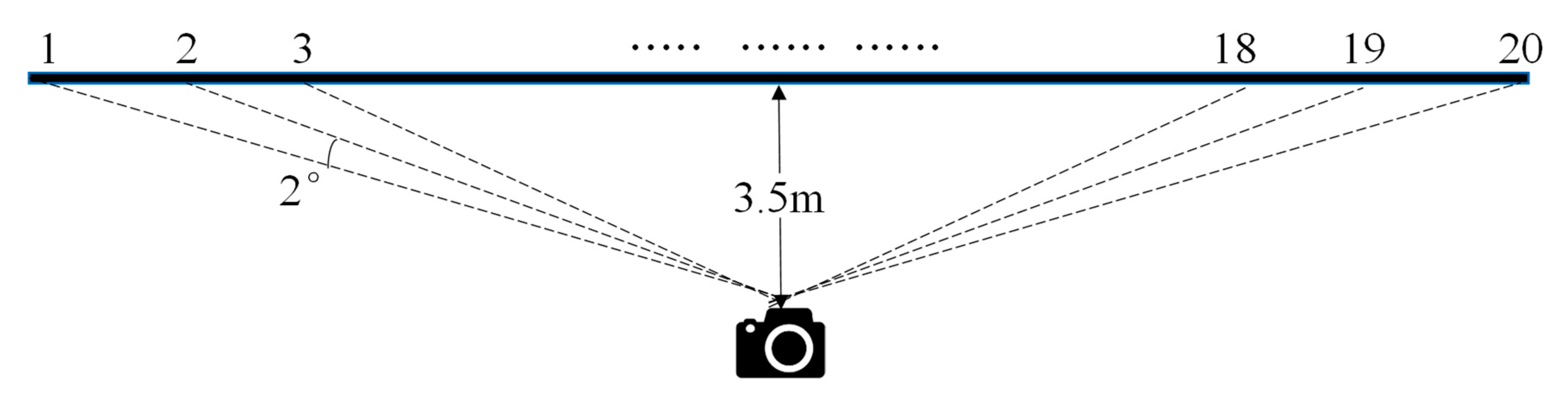
2.1.1. Image Preprocessing

Multi-view imaging of large-scale structures by rotating the camera is usually convenient. However, it is accompanied by the fact that the same structure plane has different depth of field in different images (foreshortening effects) due to the angle problem during each imaging. Only unifying the structural planes in all images can ensure no distortion in the subsequent stitching process. This can be achieved by rotating the camera imaging plane around the intersection of the optical axis and the imaging plane to be parallel to the structure plane.

This paper proposes the use of perspective transformation to re-project the original camera imaging surface to a new structure plane. The homography matrix is usually used to describe the transformation between these two-dimensional planes. The homography matrix can be solved by finding the coordinates of four points in the old and new images. Since the rotation vector and translation vector can be measured when the camera takes multi-view images, the corresponding new coordinates of the four points can be calculated based on these two vectors to achieve image preprocessing.

2.1.2. Image Registration

The preprocessed image needs to be stitched into a full-field image after removing the interference factors. Usually, the feature points of each image are calculated based on feature point detection algorithms, and the same feature points in the two images are matched with each other to calculate the homography matrix representing the transformation. Due to the different external conditions during image shooting, the overlapping areas of adjacent images will also be different, the image fusion method is needed to make the stitching effect more natural.

In this paper, the scale-invariant feature transform (SIFT) algorithm [40] is used to detect local feature points in the image. SIFT features still show good feature detection results and strong robustness even in complex environments, such as scale changes, image rotation, and brightness changes. The SIFT algorithm will simultaneously generate the coordinates of the feature points and the corresponding descriptors. For two feature points with descriptors of Q = (r₁, r₂, …, r_n) and S = (s₁, s₂, …, s_n), the Euclidean distance is calculated to evaluate their similarity.

The fast library for approximate nearest neighbors (FLANN) is used to match the feature point sets in two adjacent images. Using the K-D (k-dimensional) tree, all the feature points in the image are divided into left and right sub-tree spaces according to the root nodes of different dimensions. Then, the root nodes are determined in the sub-tree space, and the space is divided again until the space is empty, namely, all the feature points are divided. After using FLANN, there will inevitably be mismatches. If it is included in the calculation of homography matrix, there will be apparent errors in splicing. In this paper, random sample consensus (RANSAC) algorithm [41] is used to filter and only retain the correct matching feature points. The direct average fusion method is used to recalculate and replace the pixel value of the overlapping area using the average pixel value of adjacent images.

2.1.3. Structure Foreground Segmentation

Structure full-field image includes not only the structure itself, but also inevitably includes sensors, bearings, background interference, etc. However, the displacement field of the structure is only generated in the structure itself, and the other objects must be removed. Therefore, this paper uses the GrabCut algorithm [42] to extract the foreground that contains only structures.

The GrabCut algorithm is an improvement of the GraphCut algorithm [43], which is mainly reflected in the following aspects. First, to simplify the user interaction operation, we only need to roughly mark the rectangular box containing the foreground object, and the outside of the box is the background. Second, rather than gray histogram, Gaussian mixture model (GMM) is used to estimate the probability of pixels belonging to the foreground and background, and the calculation results are more reliable and accurate. Third, segmentation is not a one-time completion; therefore, through continuous iteration, we update the calculation parameters in order that the image segmentation quality is improved. After users mark the bounding box, all pixels outside the box belong entirely to the background, and the pixels inside the box may belong to both the foreground and background. Therefore, it is only necessary to segment the connection relationship between pixels in the box to separate the foreground and background.

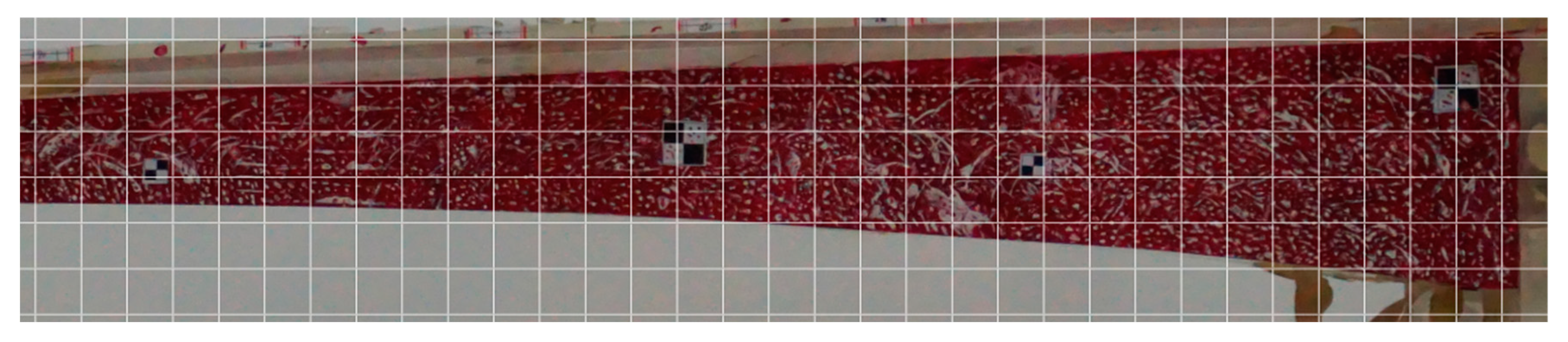
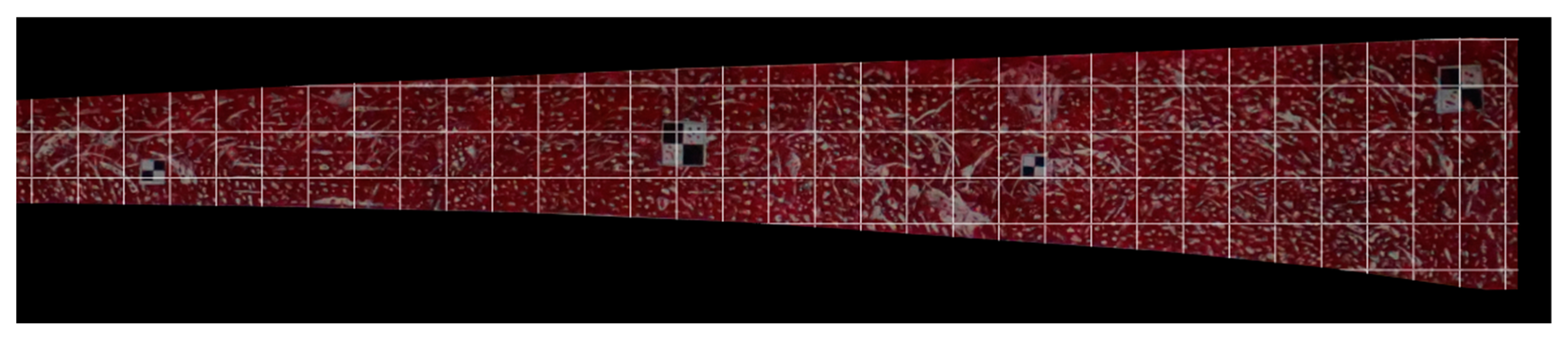
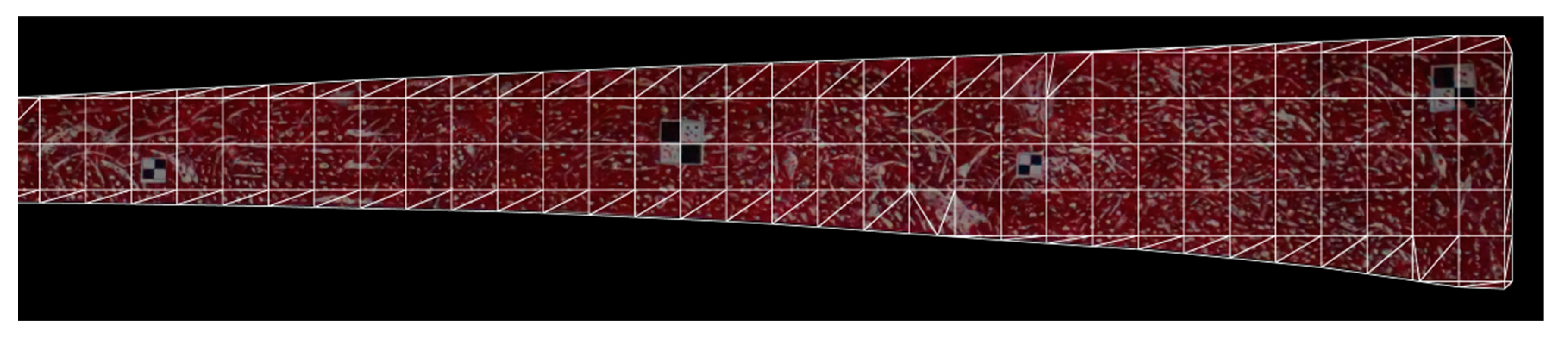
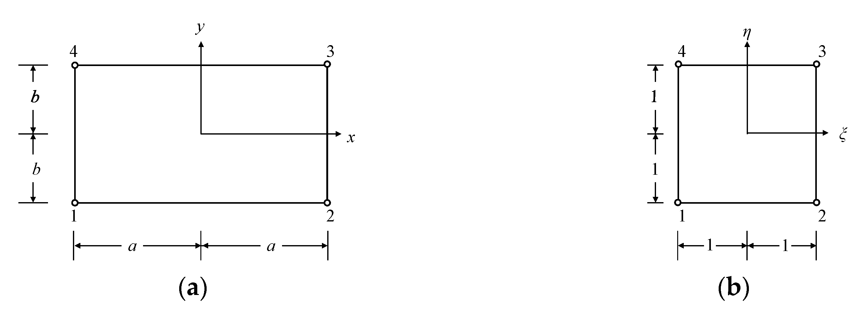
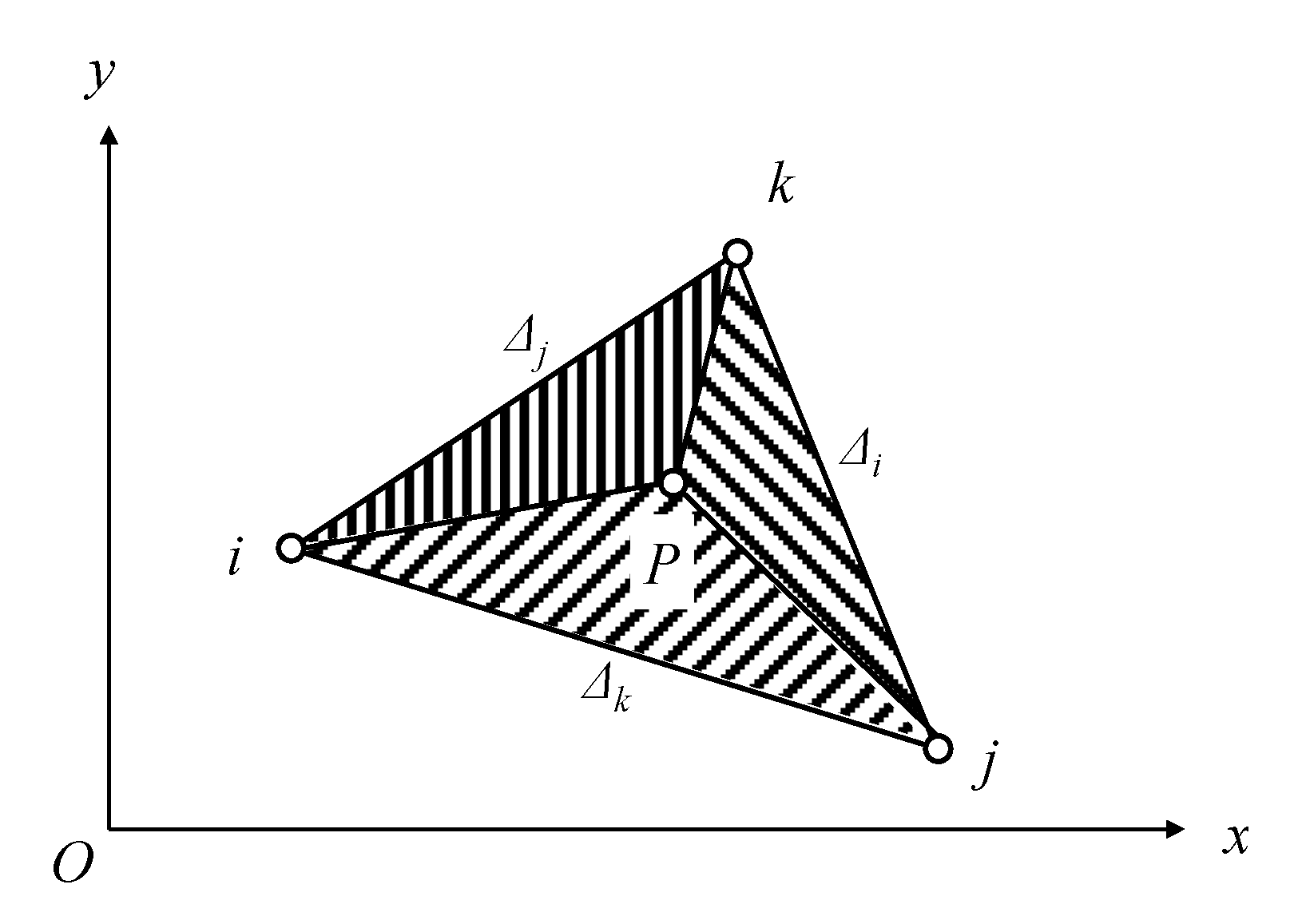
2.2. Structure Image Discretization and Displacement Field Calculation

Based on the finite element concept in the physical model, the proposed computer vision-based structural displacement field calculation with physical constraints can be divided into three steps: First, the continuous structural foreground image is discretized, and the mesh is drawn within the foreground image. The structure is divided into several regions by using the mesh. Second, the displacement of structural grid nodes is calculated based on the improved template matching method. Third, the shape function is constructed to establish the relationship between the displacement at the grid nodes and the displacement at the non-nodes in the grid, the displacement of the nodes is transferred to the non-nodes by the shape function to generate a complete displacement field. Since the shape function is a continuous function, the generated displacement field is also continuous.

2.2.1. Image Preprocessing

After determining the mesh size, the horizontal and vertical lines of the mesh are drawn on the full-field image. The grid has not abandoned the background part, which is a full-size grid, as shown in Figure 2. It is a regular rectangular grid discretization of the whole image.

Similar to foreground extraction, it is also necessary to generate the boundary of the displacement field on the full-size grid. First, the binary threshold processing is performed on the structure foreground extraction image. The background is set to 0 and the structure is set to 1 to form a binary foreground image, called a mask. To retain as many pixels as possible and ensure that the boundary of the foreground extraction has some surplus pixel space, the structure element with a kernel of 3 × 3 is used to expand the morphological processing of the binary image, and finally the expanded structure image mask is formed. Each pixel of the mask and the corresponding pixel of the full-size grid map are bitwise and calculated, namely, 1 and 1 = 1, 0 and 1 = 0, to retain the grid within the structural range. The endpoints of the above dividing line are connected to form a grid with boundary. The grid division has been initially formed, as shown in Figure 3.

The grid that does not contact the boundary is a regular rectangular grid, but the grid rules that contact the boundary are different, and further fine division needs to be completed. The grid shapes at the edge are trapezoid, pentagon, and triangle. To unify shape and refinement, the trapezoid and pentagon are divided into several triangles. To date, the division of the entire displacement field grid is completed, and the division unit has only rectangles and triangles (as shown in Figure 4), which is convenient for subsequent construction of shape functions according to the unit shape.

2.2.2. Node Displacement Calculation Using Template Matching

Template matching belongs to the digital correlation technology [2]. First, determine the template image, generate a window of the same size as the template image, and traverse the window from the upper left corner to the lower right corner in the image to be matched. Through correlation calculation, the correlation coefficient between all window images and template images is obtained, and a matrix with integer pixels is generated. The window corresponding to the peak of the correlation coefficient is the location of the template image in the image to be matched.

The core of template matching lies in the correlation calculation. The normalized sum of squared differences (NSSD) is based on the sum of squared differences to calculate the difference between the gray values of the template image and the window image pixel points. The method is simple. Although the gray value can be normalized, the effect of white noise can be weakened, but the amount of computation is quite large and it is very sensitive to illumination. The normalized cross-correlation function (NCC) is to multiply the pixel values of points on the same pixel coordinates of two images of equal size, and then compare them with the square sum root of the pixel values of all pixels of the two images. Since in the calculation process, all the pixel values are squared and then the root number is processed, which can well weaken the influence of image white noise. Although the normalized cross-correlation function can resist white noise, it cannot solve the problem of brightness inconsistency. When the same pattern is in different brightness environments, the normalized cross-correlation function calculated similarity is very low. Therefore, to solve this shortcoming, the zero-mean normalized cross-correlation function (ZNCC) is improved based on the normalized cross-correlation function named R (x, y) (shown in Equations (1) and (2)). In the calculation process, the pixel value of all pixels ($S^{x,y}(m,n)$)is subtracted from the average value of the image pixel value ($S_{av}^{x,y}$), thereby weakening the influence of the image brightness on the calculation result. In Equations (1) and (2), M and N are the height and width of the template image, m, n, x, and y are parameters, T (m, n) is the gray value, and T_av is the average gray value.

$$R(x,y)=\frac{{\displaystyle \sum _{m=1}^M{\displaystyle \sum _{n=1}^N\left\{\left[S^{x,y}\left(m,n\right)-S_{av}^{x,y}\right]\left[T\left(m,n\right)-T_{av}\right]\right\}}}}{\sqrt{{{\displaystyle \sum _{m=1}^M{\displaystyle \sum _{n=1}^N\left[S^{x,y}\left(m,n\right)-S_{av}^{x,y}\right]}}}^2}\cdot \sqrt{{{\displaystyle \sum _{m=1}^M{\displaystyle \sum _{n=1}^N\left[T\left(m,n\right)-T_{av}\right]}}}^2}}$$

(1)

$$S_{av}^{x,y}=\frac{1}{MN}{\displaystyle \sum _{m=1}^M{\displaystyle \sum _{n=1}^N{S}^{x,y}\left(m,n\right)}},T_{av}^{}=\frac{1}{MN}{\displaystyle \sum _{m=1}^M{\displaystyle \sum _{n=1}^{N}T\left(m,n\right)}}$$

(2)

2.2.3. Non-Node Displacement Calculation Using Shape Function

For non-node displacement, it is necessary to transfer the node displacement to each grid element by means of the idea of finite element shape function in the physical model [44]. Triangular and rectangular element shape functions are constructed according to the element types of the previous mesh generation results.

(1) Rectangular bilinear element shape function.

The rectangular element has four nodes; therefore, the analysis model of rectangular bilinear element is adopted, and there are eight node displacement parameters. To simplify the results, the rectangular coordinates are transformed into regular coordinates for analysis by means of coordinate transformation, as shown in Figure 5.

In the regular coordinate system, the boundary line equation of rectangular element is:

$$\{\begin{array}{c}\eta +1=0\\ \xi -1=0\\ \eta -1=0\\ \xi +1=0\end{array}$$

(3)

According to the property that the shape function Ni is 1 at node i and 0 at other points, the following equation can be acquired:

$$\{\begin{array}{c}{N}_i({\xi }_i,{\eta }_i)=1\hfill \\ N_i({\xi }_j,{\eta }_j)=0,i\ne j\end{array}$$

(4)

The shape function of each point can be set as:

$$\{\begin{array}{c}{N}_1=\alpha (\xi -1)(\eta -1)\\ N_2=\beta (\xi +1)(\eta -1)\\ N_3=\gamma (\xi +1)(\eta +1)\\ N_4=\delta (\xi -1)(\eta +1)\end{array}$$

(5)

Substituting Equation (4) into Equation (5) yields:

$$\alpha =-\beta =\gamma =-\delta =\frac{1}{4}$$

(6)

Given the displacement u_i of each node i, the displacement function of each point in the element is:

$$u(\xi ,\eta )={\displaystyle \sum N_i{u}_i}$$

(7)

(2) Triangular element shape function.

Since the shape function of triangular element in the rectangular coordinate system will be more complex, the area coordinate is introduced for analysis.

As shown in Figure 6, i, j, k are triangular element nodes, and P is any point in the element, which is connected to each node. Then, Δ_ijk is divided into three parts, which are denoted as:

$$\{\begin{array}{c}{\mathrm{\Delta }}_i=\mathrm{\Delta }Pjk\hfill \\ {\mathrm{\Delta }}_j=\mathrm{\Delta }Pki\hfill \\ {\mathrm{\Delta }}_k=\mathrm{\Delta }Pij\hfill \\ \mathrm{\Delta }={\mathrm{\Delta }}_i+{\mathrm{\Delta }}_j+{\mathrm{\Delta }}_k=\mathrm{\Delta }ijk\hfill \end{array}$$

(8)

The position of point P can be represented by rectangular coordinates, and can also be represented by Δ_i, Δ_j, Δ_k.

$$L_l=\frac{{\mathrm{\Delta }}_l}{\mathrm{\Delta }}(l=i,j,k)$$

(9)

Then, the position of point P can also be determined by L_l, which is called area coordinate.

Let the point P coordinate be (x, y), then the area divided into three parts is:

$${\mathrm{\Delta }}_i=\frac{1}{2}\left|\begin{array}{ccc}x& y& 1\\ x_j& y_j& 1\\ x_k& y_k& 1\end{array}\right|i\to j\to k\to i$$

(10)

The unit area is:

$$\mathrm{\Delta }=\frac{1}{2}\left|\begin{array}{ccc}{x}_i& y_i& 1\\ x_j& y_j& 1\\ x_k& y_k& 1\end{array}\right|$$

(11)

Therefore, the area coordinate is:

$$\begin{array}{cc}\hfill L_i& =\frac{{\mathrm{\Delta }}_i}{\mathrm{\Delta }}=\frac{1}{2\mathrm{\Delta }}\left(x\left|\begin{array}{cc}{y}_j& 1\\ y_k& 1\end{array}\right|-y\left|\begin{array}{cc}{x}_j& 1\\ x_k& 1\end{array}\right|+1\left|\begin{array}{cc}{x}_j& x_j\\ x_k& x_k\end{array}\right|\right)\hfill \\ & =\frac{1}{2\mathrm{\Delta }}\left(a_i+b_{i}x+c_{i}y\right)\left(i\to j\to k\to i\right)\hfill \end{array}$$

(12)

$$\{\begin{array}{c}{a}_i=x_j{y}_k-x_k{y}_j\hfill \\ b_i=y_j-y_k\hfill \\ c_i=x_k-x_j\hfill \end{array}\left(i\to j\to k\to i\right)$$

(13)

According to the properties of shape functions, L_i, L_j, and L_k are the shape functions of triangular elements. The displacement of each point inside the triangular element is calculated by Equation (7).

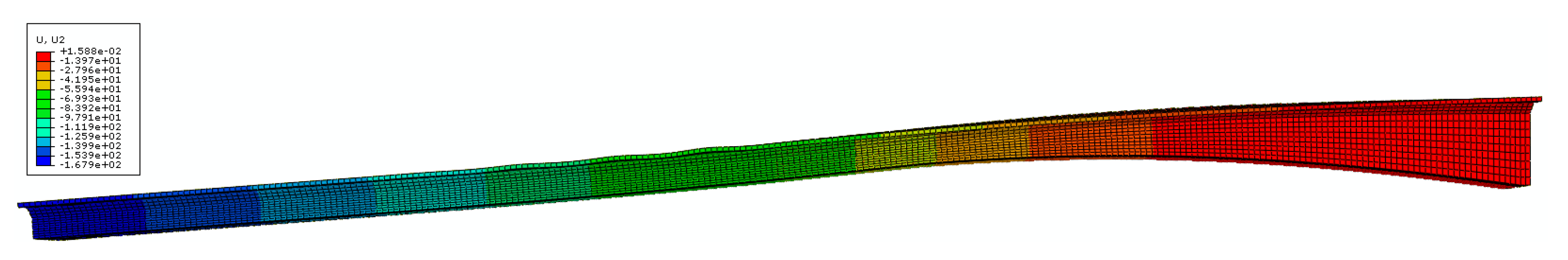
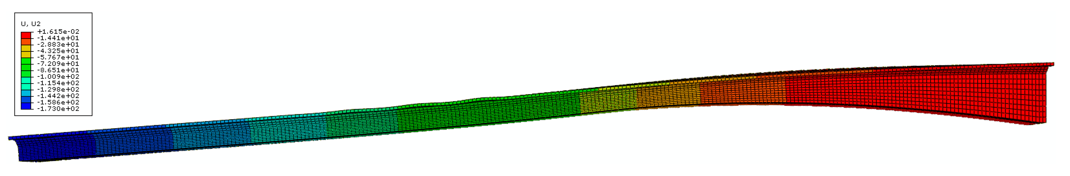
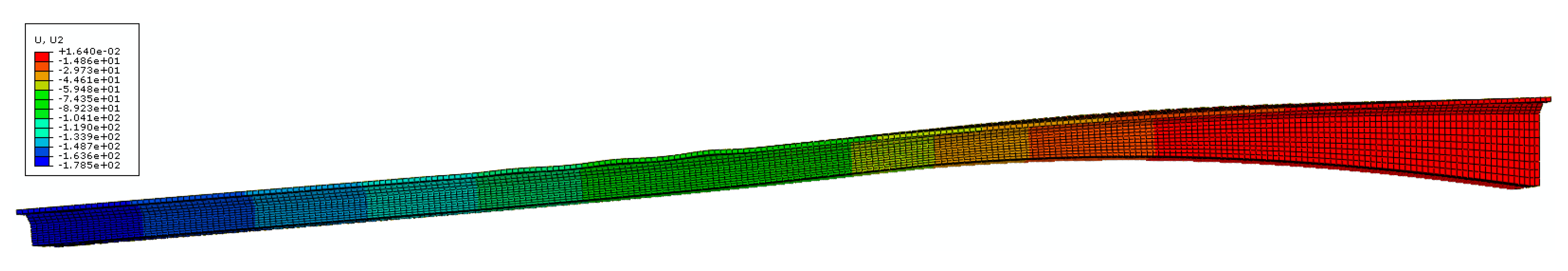
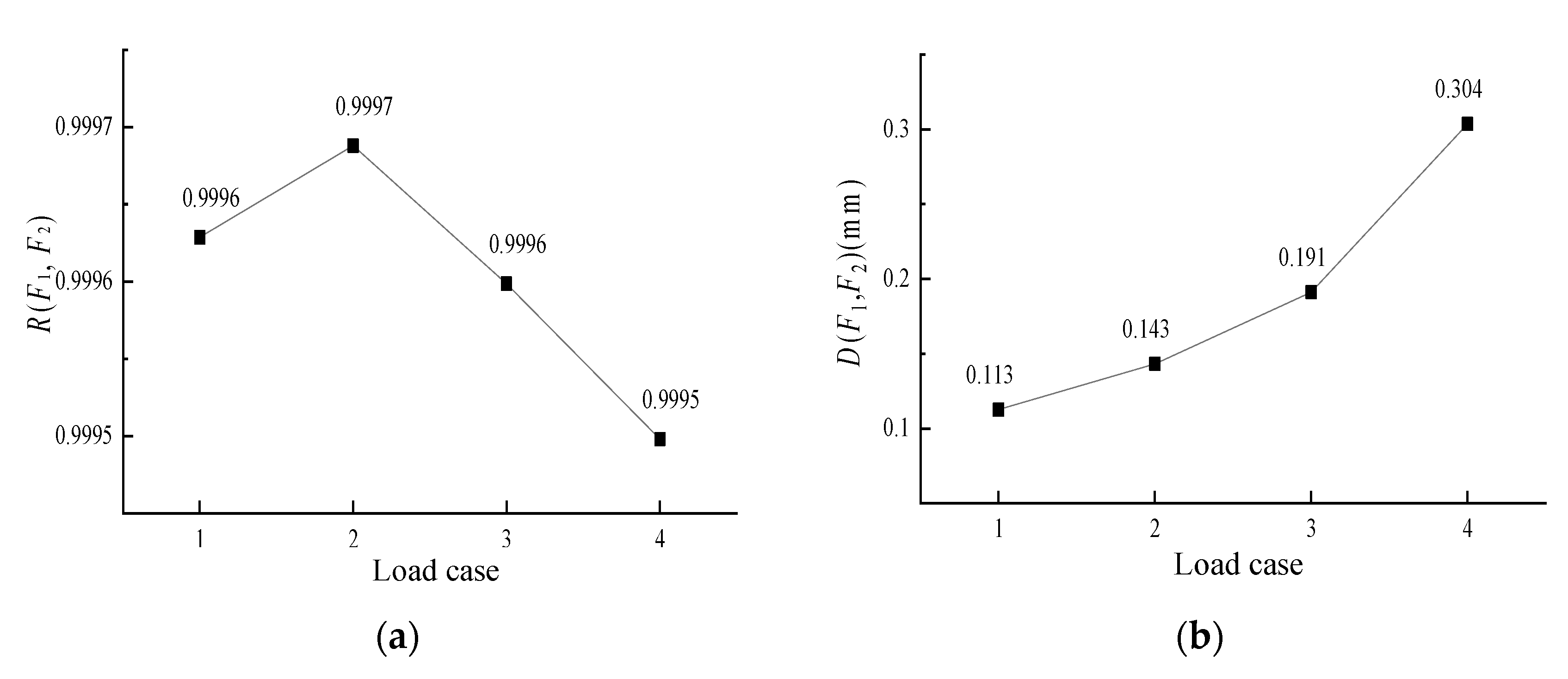
3. Validation Results and Discussion

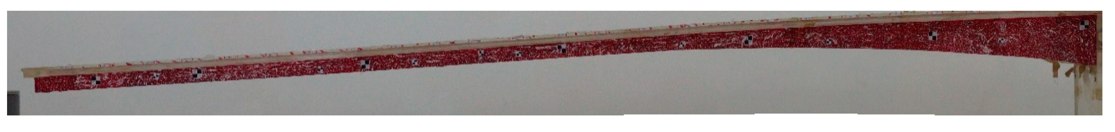
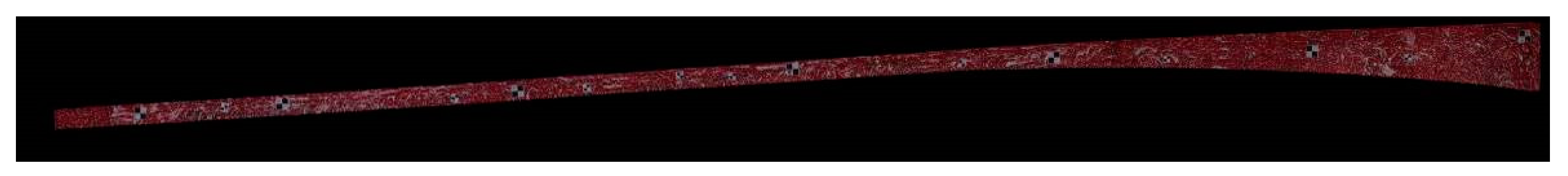
3.1. Full-Field Image Generation Results

The bridge model used in this test is a side span of organic glass three-span continuous beam. To reduce the structural stiffness, the side span pier was removed and turned into a cantilever beam structure (2644 mm long). The camera is consumer-grade (Sony α-6000) with a resolution of 6000 × 4000. The structure was photographed from left to right using a fully automatic rotating pan-tilt control platform installed on a static tripod, as shown in Figure 7. The rotation speed was 2 degrees per second, and a total of 20 structural images were obtained. To verify the accuracy of the proposed method for displacement measurement, artificial targets of known sizes (20 mm × 20 mm) were placed at 200 mm, 400 mm, 800 mm, 1300 mm, 1800 mm, and 2200 mm from the beam end, two LVDT displacement sensors were installed 400 mm and 1300 mm, respectively. Four loading cases were tested (different loadings placed at the cantilever end to excite different displacement fields of the structure were kept for 2 min, as shown in Figure 8).

The preprocessing method was used to process the obtained 20 images to eliminate the foreshortening effect. The full-field image of the structure obtained by image stitching is shown in Figure 9. The conversion coefficient represents the actual distance represented by a pixel in the image. According to the artificial target, the conversion coefficient error of each part of the whole field image is calculated to be within 1%, which shows the effectiveness of the preprocessing algorithm. The structure foreground segmentation result is shown in Figure 10.

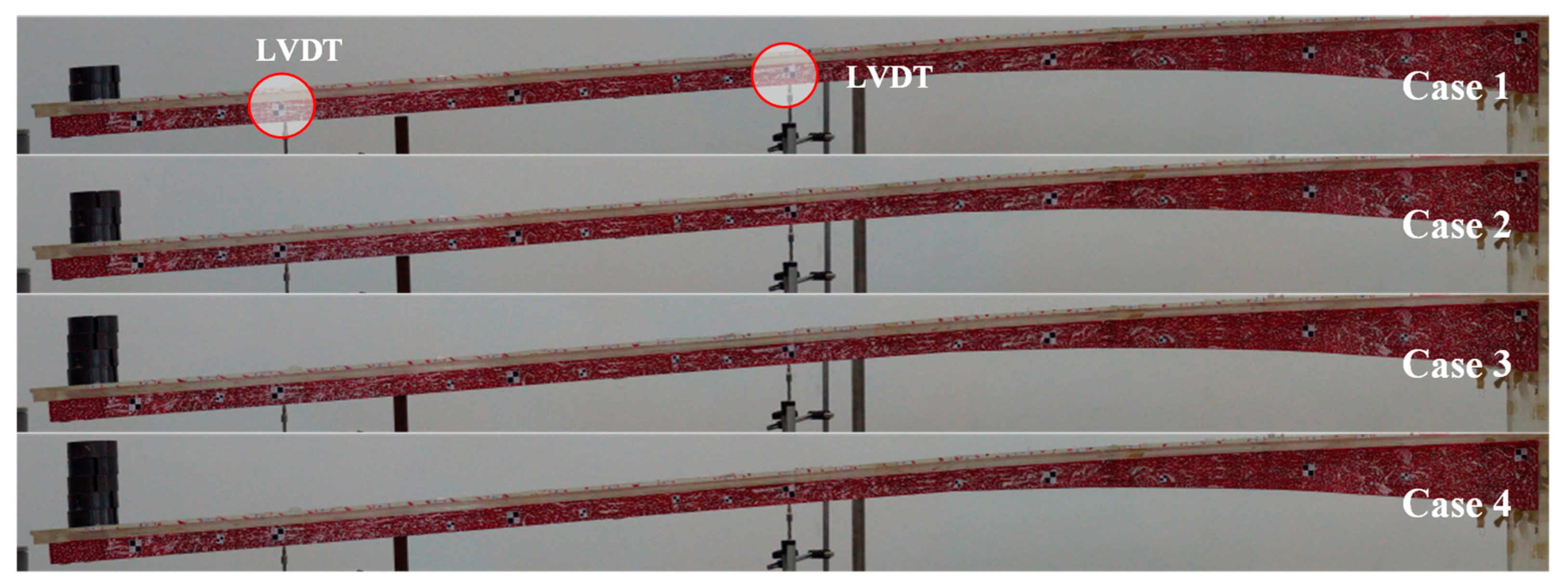
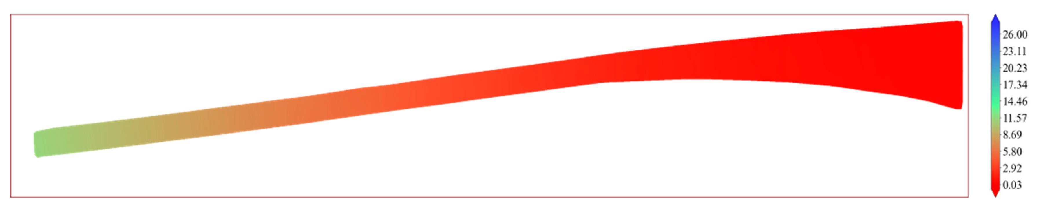
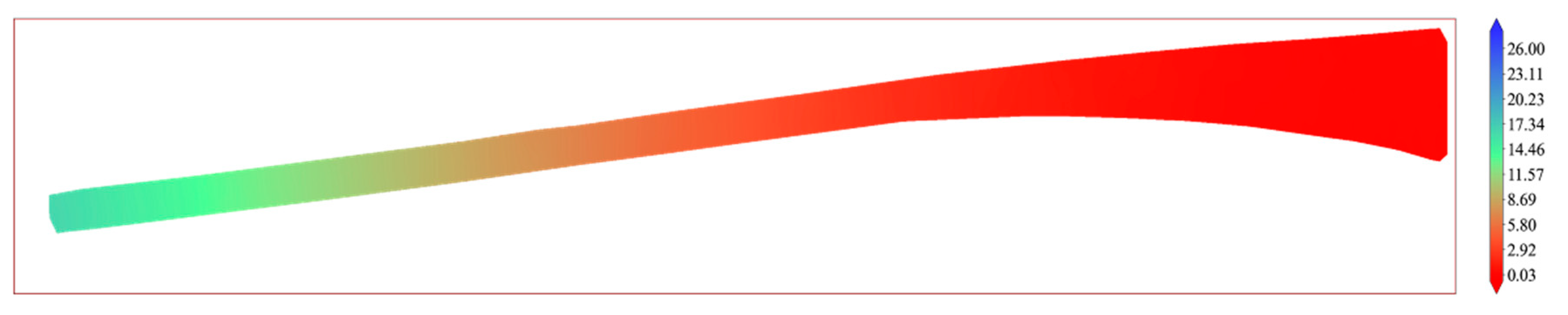
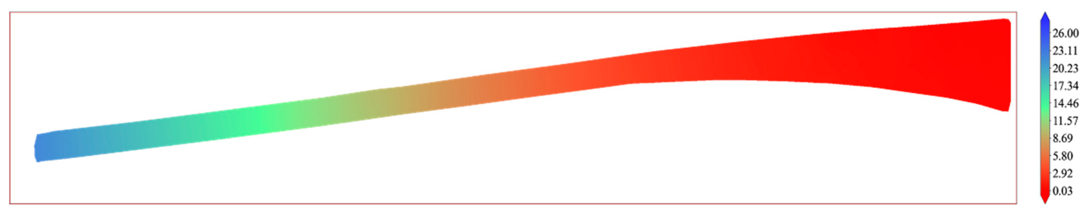
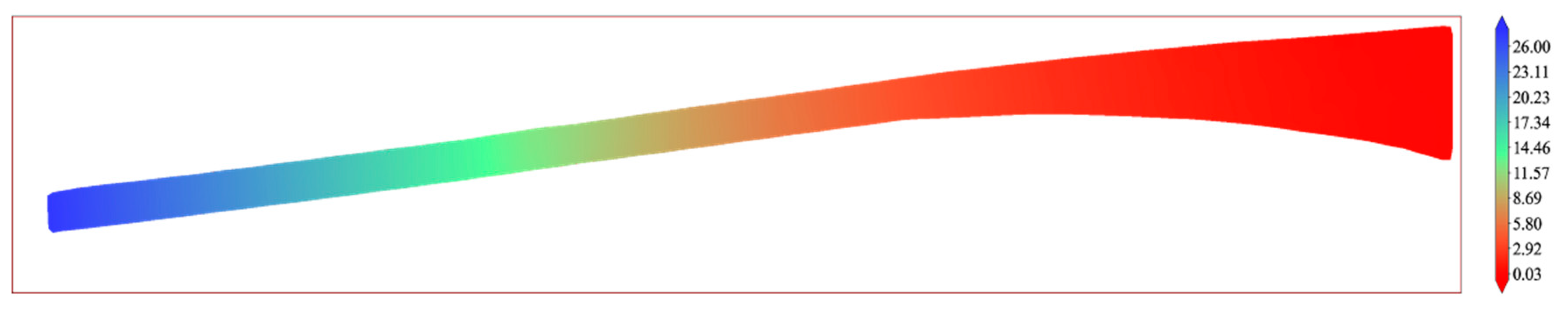
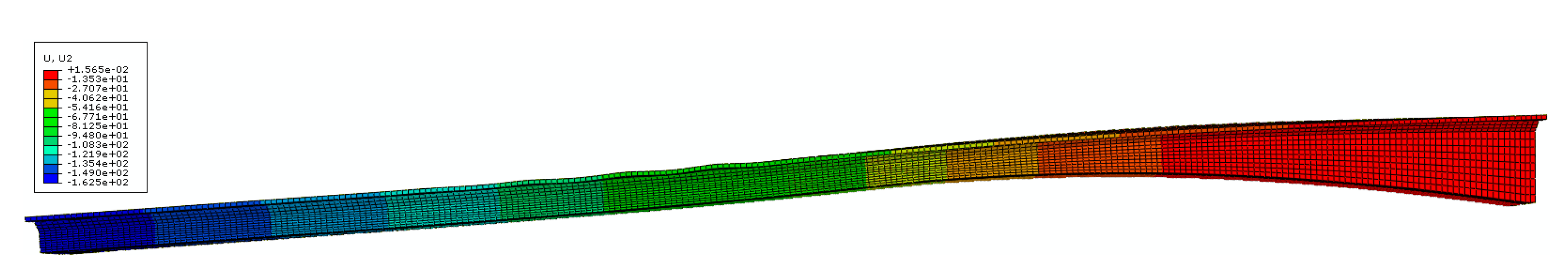
3.2. Displacement Field Calculation Results

The node displacement is calculated by the above method, and the conversion coefficient obtained by calibration is 0.073734 mm/pixel. Compared with the key point displacement of the LVDT set by 400 mm and 1300 mm, the results are shown in

Table 1. Comparison of key node displacement calculated by the proposed method and LVDT.

Loading Case	400 mm (mm)				1300 mm (mm)
	LVDT	Proposed	Error	Error (%)	LVDT	Proposed	Error	Error (%)
1	8.356	8.455	0.099	1.2	2.901	2.895	0.006	0.2
2	12.381	12.454	0.073	0.6	4.229	4.002	0.227	5.4
3	16.354	16.574	0.220	1.3	5.662	5.485	0.177	3.1
4	20.466	20.504	0.038	0.2	7.048	6.877	0.171	2.4
Average	-	-	-	0.826	-	-	-	2.7

. The maximum node displacement error calculated by the proposed method is 5.4%, which shows the effectiveness and accuracy of the proposed method.

In the generated full-field image, the lowest of the bridge structure is about 500 pixels, and the highest is about 1600 pixels. The size of the template in template matching technique is set to 81 × 81, and the mesh size is set to 400 × 400. With the initial state image as a reference, the proposed method was used to calculate the structural displacement field for four loading cases, and the results are shown in Figure 11, Figure 12, Figure 13 and Figure 14. The calculated structural displacement field conforms to the law of structural mechanics and the displacement change is continuous, which can preliminarily validate the feasibility of the proposed method.

To quantitatively evaluate the accuracy of the structural displacement field calculated by the proposed method, the corresponding finite element model was established and updated according to the geometric size and material properties of the bridge model used in the experiment (the objective is the displacement difference at the position of LVDT). The bridge material is plexiglass, the density is 1155 kg/m³, the elastic modulus is 2.2 GPa, and the Poisson’s ratio is 0.38. When meshing the model, the cutting plane is defined per 10 mm from the cantilever end, and the web plate height direction has 10 nodes, as shown in Figure 15.

The distance from the cantilever end to the 2600 mm on the side of the web plate is also 10 × 261 = 2610 nodes. The consolidation end of the model is completely consolidated, and the displacement load is applied to the section at 400 mm and 1300 mm from the cantilever end to simulate the actual load. The finite element software Abaqus was used to simulate the displacement field corresponding to the initial state and four working conditions, the displacement fields calculated by the finite element model are shown in Figure 16, Figure 17, Figure 18 and Figure 19. Considering the displacement field dimension calculated by the proposed method, the corresponding displacement fields of different load cases generated by the finite element model are extracted.

To evaluate the similarity of two displacement fields (F₁, F₂), the normalized correlation coefficient R (F₁, F₂) is proposed as the evaluation index. The calculation method is shown in Equation (14), where M and N are the number of rows and columns of the displacement field, and F (m, n) is the displacement value at the position of the displacement field (m, n). In addition, the deviation between data is an important index to measure the difference of displacement field. The difference between two displacement field data is defined as the root mean square deviation D (F₁, F₂), and its calculation method is shown in Equation (15).

$$R(F_1,F_2)=\frac{{\displaystyle \sum _{m=1}^M{\displaystyle \sum _{n=1}^N\left[F_1\left(m,n\right)\cdot F_2\left(m,n\right)\right]}}}{\sqrt{{{\displaystyle \sum _{m=1}^M{\displaystyle \sum _{n=1}^N\left[F_1\left(m,n\right)\right]}}}^2}\cdot \sqrt{{{\displaystyle \sum _{m=1}^M{\displaystyle \sum _{n=1}^N\left[F_2\left(m,n\right)\right]}}}^2}}$$

(14)

$$D(F_1,F_2)=\sqrt{\frac{{\displaystyle \sum _{m=1}^M{\displaystyle \sum _{n=1}^N\left[{\left(F_1\left(m,n\right)-F_2\left(m,n\right)\right)}^2\right]}}}{M\times N}}$$

(15)

Figure 20 shows the quantitative evaluation results of the structural displacement field under different load conditions calculated by the proposed method. The R values of the calculation results of the proposed method and the finite element model are higher than 0.9995, indicating that the overall trend of the calculated displacement field is similar to the real displacement field. The D values are all less than 0.304 mm, and the relative offset obtained by dividing the D value by the maximum displacement field of the four load cases is less than 1.2%, which verifies the accuracy of the proposed method.

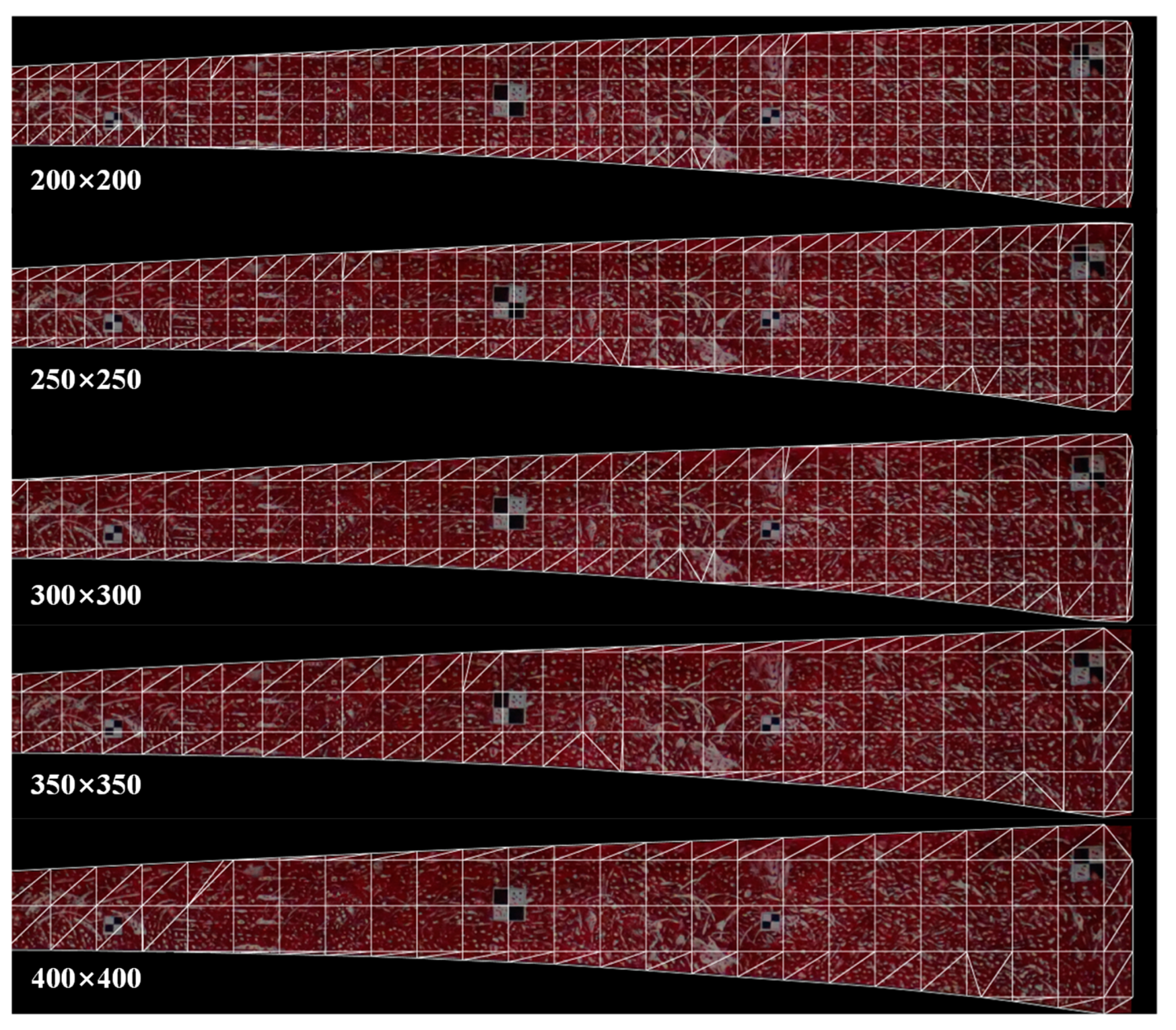
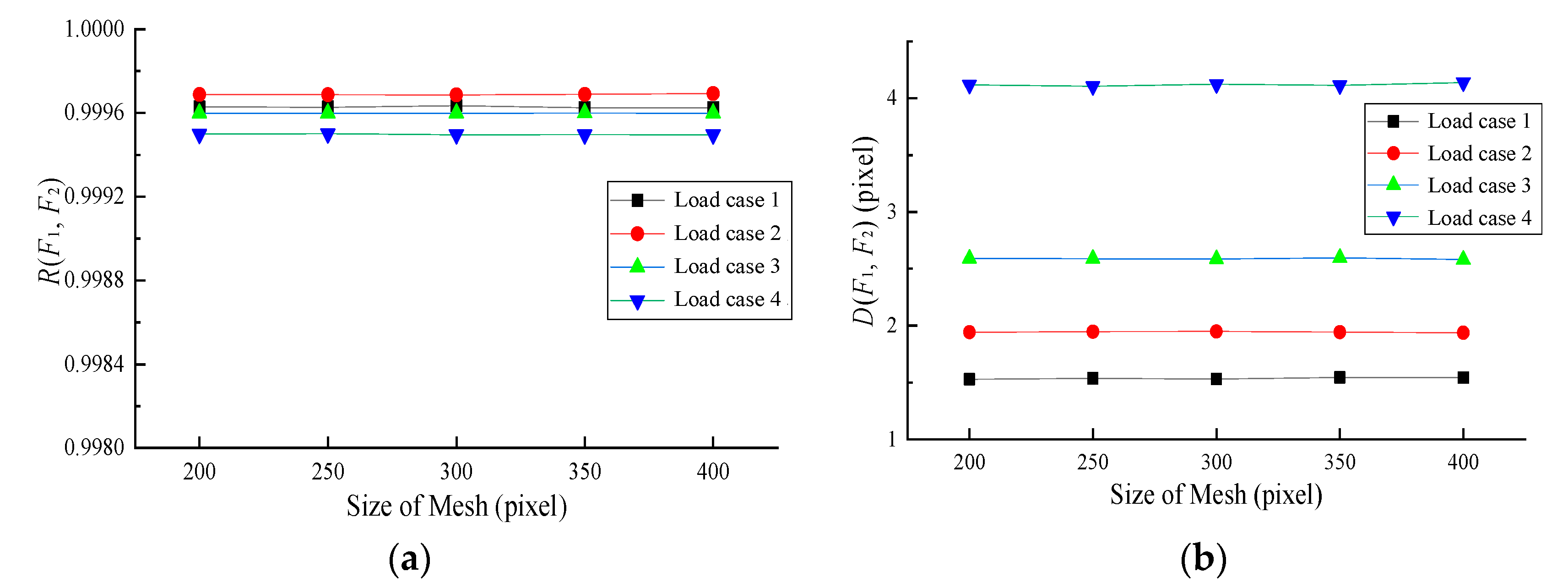
3.3. The Influence of Different Mesh Sizes

As one of the important parameters of the proposed method, the mesh size affects the number of meshes and nodes in the full-field structural image. In the full-field bridge image of this experiment, the minimum structural height is only 500 pixels, and thus the mesh size should not be greater than 500. To study the influence of mesh size on the calculation of structural displacement field, five different meshes of 200 × 200, 250 × 250, 300 × 300, 350 × 350, and 400 × 400 were used to divide the image. The local meshes near the consolidation end are shown in Figure 21.

The R and D values of the structural displacement field calculated with different mesh sizes are calculated, respectively. The results are shown in Figure 22. The R and D values corresponding to the five mesh sizes are basically unchanged, which verifies that the mesh size has no significant effect on the calculation accuracy of the structural displacement field. However, considering that the larger the mesh size, the fewer the number of generated mesh and nodes, namely, the higher the calculation efficiency, it is recommended that the mesh size can be as large as possible within the allowable range. Therefore, the selection principle of grid size is to ensure that the maximum grid size is based on ensuring at least one complete grid in the short side direction of the structure.

4. Conclusions

In this paper, a displacement field calculation framework of large-scale structures based on computer vision with physical constraints is proposed. Only a single camera is used to solve the contradiction between imaging field-of-view and resolution, and the accurate acquisition of large-scale structural displacement field is realized. The specific conclusions can be drawn as follows. It is feasible to use the camera set on the automatic rotating device to obtain high-resolution images of large-scale structures, and then use image stitching technology to generate panoramic images of structures. The laboratory bridge model (2644 mm long) is used to verify the proposed framework, and an updated finite element model is established for quantitative evaluation. The evaluation index R is greater than 0.9995, and the D value is less than 0.304 mm, which validate the accuracy of the proposed method. The parameter sensitivity analysis of mesh size, one of the important parameters, is conducted. The mesh size has no significant effect on the accuracy, but considering the computational efficiency, the mesh size can obtain the upper limit of the allowable range.

In this paper, the displacement field of a large structure is obtained at a small hardware cost, but the limitation is that it can only be used for static or quasi-static deformation of the structure, and cannot realize real-time calculation of the dynamic displacement field. This is due to the fact that the use of automatic rotating device for image shooting requires time that cannot be ignored. Future work will focus on improving the workflow of the rotating device or using multi-lens cameras for simultaneous shooting to minimize image acquisition time and further improve the efficiency of the algorithm to achieve real-time acquisition of dynamic displacement fields.

References

1. Dong, C.-Z.; Catbas, F.N. A review of computer vision–based structural health monitoring at local and global levels. Struct. Health Monit. 2020, 20, 692–743. [Google Scholar] [CrossRef]
2. Feng, D.; Feng, M.Q. Experimental validation of cost-effective vision-based structural health monitoring. Mech. Syst. Signal Process. 2017, 88, 199–211. [Google Scholar] [CrossRef]
3. Liu, Y.; Li, Y.; Wang, D.; Zhang, S. Model Updating of Complex Structures Using the Combination of Component Mode Synthesis and Kriging Predictor. Sci. World J. 2014, 2014, 476219. [Google Scholar] [CrossRef]
4. Liu, Y.; Zhang, S. Damage Localization of Beam Bridges Using Quasi-Static Strain Influence Lines Based on the BOTDA Technique. Sensors 2018, 18, 4446. [Google Scholar] [CrossRef] [PubMed]
5. Cha, Y.J.; Choi, W.; Büyüköztürk, O. Deep learning-based crack damage detection using convolutional neural networks. Comput. -Aided Civil. Infrastruct. Eng. 2017, 32, 361–378. [Google Scholar] [CrossRef]
6. Kong, X.; Li, J. Vision-based fatigue crack detection of steel structures using video feature tracking. Comput. -Aided Civil. Infrastruct. Eng. 2018, 33, 783–799. [Google Scholar] [CrossRef]
7. Ramana, L.; Choi, W.; Cha, Y.-J. Fully automated vision-based loosened bolt detection using the Viola–Jones algorithm. Struct. Health Monit. 2018, 18, 422–434. [Google Scholar] [CrossRef]
8. Xu, Y.; Li, S.; Zhang, D.; Jin, Y.; Zhang, F.; Li, N.; Li, H. Identification framework for cracks on a steel structure surface by a restricted Boltzmann machines algorithm based on consumer-grade camera images. Struct. Control. Health Monit. 2018, 25, e2075. [Google Scholar] [CrossRef]
9. Bao, Y.; Shi, Z.; Beck, J.L.; Li, H.; Hou, T.Y. Identification of time-varying cable tension forces based on adaptive sparse time-frequency analysis of cable vibrations. Struct. Control. Health Monit. 2017, 24, e1889. [Google Scholar] [CrossRef]
10. Huang, Y.; Beck, J.L.; Li, H. Bayesian system identification based on hierarchical sparse Bayesian learning and Gibbs sampling with application to structural damage assessment. Comput. Methods Appl. Mech. Eng. 2017, 318, 382–411. [Google Scholar] [CrossRef]
11. Li, H.; Lan, C.M.; Ju, Y.; Li, D.S. Experimental and Numerical Study of the Fatigue Properties of Corroded Parallel Wire Cables. J. Bridge Eng. 2012, 17, 211–220. [Google Scholar] [CrossRef]
12. Li, H.; Mao, C.-X.; Ou, J.-P. Experimental and theoretical study on two types of shape memory alloy devices. Earthq. Eng. Struct. Dyn. 2008, 37, 407–426. [Google Scholar] [CrossRef]
13. Li, S.; Wei, S.; Bao, Y.; Li, H. Condition assessment of cables by pattern recognition of vehicle-induced cable tension ratio. Eng. Struct. 2018, 155, 1–15. [Google Scholar] [CrossRef]
14. Li, S.; Zhu, S.; Xu, Y.-L.; Chen, Z.-W.; Li, H. Long-term condition assessment of suspenders under traffic loads based on structural monitoring system: Application to the Tsing Ma Bridge. Struct. Control. Health Monit. 2012, 19, 82–101. [Google Scholar] [CrossRef]
15. Sony, S.; Laventure, S.; Sadhu, A. A literature review of next-generation smart sensing technology in structural health monitoring. Struct. Control. Health Monit. 2019, 26, e2321. [Google Scholar] [CrossRef]
16. Spencer, B.F.; Hoskere, V.; Narazaki, Y. Advances in Computer Vision-Based Civil Infrastructure Inspection and Monitoring. Engineering 2019, 5, 199–222. [Google Scholar] [CrossRef]
17. Bernasconi, A.; Carboni, M.; Comolli, L.; Galeazzi, R.; Gianneo, A.; Kharshiduzzaman, M. Fatigue Crack Growth Monitoring in Composite Bonded Lap Joints by a Distributed Fibre Optic Sensing System and Comparison with Ultrasonic Testing. J. Adhes. 2016, 92, 739–757. [Google Scholar] [CrossRef]
18. Zamani, P.; Jaamialahmadi, A.; da Silva, L.F.M.; Farhangdoost, K. An investigation on fatigue life evaluation and crack initiation of Al-GFRP bonded lap joints under four-point bending. Compos. Struct. 2019, 229, 111433. [Google Scholar] [CrossRef]
19. Moradi, A.; Shariati, M.; Zamani, P.; Karimi, R. Experimental and numerical analysis of ratcheting behavior of A234 WPB steel elbow joints including corrosion defects. Proc. Inst. Mech. Eng. Part. L J. Mater. Des. Appl. 2022, 237, 451–468. [Google Scholar] [CrossRef]
20. Zamani, P.; Fm da Silva, L.; Masoudi Nejad, R.; Ghahremani Moghaddam, D.; Soltannia, B. Experimental study on mixing ratio effect of hybrid graphene nanoplatelet/nano-silica reinforcement on the static and fatigue life of aluminum-to-GFRP bonded joints under four-point bending. Compos. Struct. 2022, 300, 116108. [Google Scholar] [CrossRef]
21. Djabali, A.; Toubal, L.; Zitoune, R.; Rechak, S. Fatigue damage evolution in thick composite laminates: Combination of X-ray tomography, acoustic emission and digital image correlation. Compos. Sci. Technol. 2019, 183, 107815. [Google Scholar] [CrossRef]
22. Feng, D.; Feng, M.Q. Computer vision for SHM of civil infrastructure: From dynamic response measurement to damage detection—A review. Eng. Struct. 2018, 156, 105–117. [Google Scholar] [CrossRef]
23. Xu, Y.; Brownjohn, J.M.W. Review of machine-vision based methodologies for displacement measurement in civil structures. J. Civil. Struct. Health Monit. 2018, 8, 91–110. [Google Scholar] [CrossRef]
24. Feng, D.; Feng, M.Q. Vision-based multipoint displacement measurement for structural health monitoring. Struct. Control. Health Monit. 2016, 23, 876–890. [Google Scholar] [CrossRef]
25. Aoyama, T.; Li, L.; Jiang, M.; Takaki, T.; Ishii, I.; Yang, H.; Umemoto, C.; Matsuda, H.; Chikaraishi, M.; Fujiwara, A. Vision-Based Modal Analysis Using Multiple Vibration Distribution Synthesis to Inspect Large-Scale Structures. J. Dyn. Syst. Meas. Control. 2018, 141, 031007. [Google Scholar] [CrossRef]
26. Luo, L.; Feng, M.Q.; Wu, Z.Y. Robust vision sensor for multi-point displacement monitoring of bridges in the field. Eng. Struct. 2018, 163, 255–266. [Google Scholar] [CrossRef]
27. Lydon, D.; Lydon, M.; Rincón, J.M.d.; Taylor, S.E.; Robinson, D.; O’Brien, E.; Catbas, F.N. Development and Field Testing of a Time-Synchronized System for Multi-Point Displacement Calculation Using Low-Cost Wireless Vision-Based Sensors. IEEE Sens. J. 2018, 18, 9744–9754. [Google Scholar] [CrossRef]
28. Xu, Y.; Brownjohn, J.; Kong, D. A non-contact vision-based system for multipoint displacement monitoring in a cable-stayed footbridge. Struct. Control. Health Monit. 2018, 25, e2155. [Google Scholar] [CrossRef]
29. Song, Q.S.; Wu, J.R.; Wang, H.L.; An, Y.S.; Tang, G.W. Computer vision-based illumination-robust and multi-point simultaneous structural displacement measuring method. Mech. Syst. Signal. Process. 2022, 170, 108822. [Google Scholar] [CrossRef]
30. Lai, Z.; Alzugaray, I.; Chli, M.; Chatzi, E. Full-field structural monitoring using event cameras and physics-informed sparse identification. Mech. Syst. Signal. Process. 2020, 145, 106905. [Google Scholar] [CrossRef]
31. Shang, Z.; Shen, Z. Multi-point vibration measurement and mode magnification of civil structures using video-based motion processing. Autom. Constr. 2018, 93, 231–240. [Google Scholar] [CrossRef]
32. Yang, Y.; Dorn, C.; Farrar, C.; Mascarenas, D. Blind, simultaneous identification of full-field vibration modes and large rigid-body motion of output-only structures from digital video measurements. Eng. Struct. 2020, 207, 110183. [Google Scholar] [CrossRef]
33. Yang, Y.; Sanchez, L.; Zhang, H.; Roeder, A.; Bowlan, J.; Crochet, J.; Farrar, C.; Mascarenas, D. Estimation of full-field, full-order experimental modal model of cable vibration from digital video measurements with physics-guided unsupervised machine learning and computer vision. Struct. Control. Health Monit. 2019, 26, e2358. [Google Scholar] [CrossRef]
34. Narazaki, Y.; Gomez, F.; Hoskere, V.; Smith, M.D.; Spencer, B.F. Efficient development of vision-based dense three-dimensional displacement measurement algorithms using physics-based graphics models. Struct. Health Monit. Int. J. 2021, 20, 1841–1863. [Google Scholar] [CrossRef]
35. Narazaki, Y.; Hoskere, V.; Eick, B.A.; Smith, M.D.; Spencer, B.F. Vision-based dense displacement and strain estimation of miter gates with the performance evaluation using physics-based graphics models. Smart Struct. Syst. 2019, 24, 709–721. [Google Scholar] [CrossRef]
36. Bhowmick, S.; Nagarajaiah, S. Identification of full-field dynamic modes using continuous displacement response estimated from vibrating edge video. J. Sound Vib. 2020, 489, 115657. [Google Scholar] [CrossRef]
37. Bhowmick, S.; Nagarajaiah, S. Spatiotemporal compressive sensing of full-field Lagrangian continuous displacement response from optical flow of edge: Identification of full-field dynamic modes. Mech. Syst. Signal. Process. 2022, 164, 108232. [Google Scholar] [CrossRef]
38. Bhowmick, S.; Nagarajaiah, S.; Lai, Z. Measurement of full-field displacement time history of a vibrating continuous edge from video. Mech. Syst. Signal. Process. 2020, 144, 106847. [Google Scholar] [CrossRef]
39. Luan, L.; Zheng, J.; Wang, M.L.; Yang, Y.; Rizzo, P.; Sun, H. Extracting full-field subpixel structural displacements from videos via deep learning. J. Sound. Vib. 2021, 505, 116142. [Google Scholar] [CrossRef]
40. Cheung, W.; Hamarneh, G. n-SIFT: N-dimensional scale invariant feature transform. Trans. Img. Proc. 2009, 18, 2012–2021. [Google Scholar] [CrossRef]
41. Fischler, M.A.; Bolles, R.C. Random sample consensus: A paradigm for model fitting with applications to image analysis and automated cartography. Commun. ACM 1981, 24, 381–395. [Google Scholar] [CrossRef]
42. Rother, C.; Kolmogorov, V.; Blake, A. “GrabCut”: Interactive foreground extraction using iterated graph cuts. In Proceedings of the SIGGRAPH 2004: 31st Annual Conference on Computer Graphics and Interactive Techniques, Los Angeles, CA, USA, 8–12 August 2004; pp. 309–314. [Google Scholar]
43. Vicente, S.; Kolmogorov, V.; Rother, C. Graph cut based image segmentation with connectivity priors. In Proceedings of the 2008 IEEE Conference on Computer Vision and Pattern Recognition, Anchorage, AK, USA, 23–28 June 2008; pp. 1–8. [Google Scholar]
44. Stevenson, R. Optimality of a Standard Adaptive Finite Element Method. Found. Comput. Math. 2007, 7, 245–269. [Google Scholar] [CrossRef]
Figure 1. Overall framework of the proposed structural displacement field calculation method.
Sustainability 15 08683 g001
Figure 2. Full-size grid of the full-field structure image.
Sustainability 15 08683 g002
Figure 3. Structure region grid of the full-field structure image.
Sustainability 15 08683 g003
Figure 4. Final grid of the full-field structure image.
Sustainability 15 08683 g004
Figure 5. Rectangular bilinear element: (a) Cartesian coordinate system; (b) regular coordinate system.
Sustainability 15 08683 g005
Figure 6. Area coordinate of triangular element.
Sustainability 15 08683 g006
Figure 7. Schematic diagram of the rotation shooting process.
Sustainability 15 08683 g007
Figure 8. Four different loading cases.
Sustainability 15 08683 g008
Figure 9. Full-field image of the structure obtained by image stitching.
Sustainability 15 08683 g009
Figure 10. Structure foreground segmentation result.
Sustainability 15 08683 g010
Figure 11. Calculated structural displacement field for Case 1.
Sustainability 15 08683 g011
Figure 12. Calculated structural displacement field for Case 2.
Sustainability 15 08683 g012
Figure 13. Calculated structural displacement field for Case 3.
Sustainability 15 08683 g013
Figure 14. Calculated structural displacement field for Case 4.
Sustainability 15 08683 g014
Figure 15. Finite element model of the employed bridge model.
Sustainability 15 08683 g015
Figure 16. Calculated structural displacement field by the finite element model for Case 1.
Sustainability 15 08683 g016
Figure 17. Calculated structural displacement field by the finite element model for Case 2.
Sustainability 15 08683 g017
Figure 18. Calculated structural displacement field by the finite element model for Case 3.
Sustainability 15 08683 g018
Figure 19. Calculated structural displacement field by the finite element model for Case 4.
Sustainability 15 08683 g019
Figure 20. Quantitative evaluation results of the structural displacement field: (a) R (F1, F2); (b) D (F1, F2).
Sustainability 15 08683 g020
Figure 21. Local meshes near the consolidation end with different mesh sizes.
Sustainability 15 08683 g021
Figure 22. Quantitative evaluation results with different mesh sizes: (a) R (F1, F2); (b) D (F1, F2).
Sustainability 15 08683 g022