Control of Oxygen Excess Ratio for a PEMFC Air Supply System by Intelligent PID Methods

Abstract

The hydrogen fuel cell is a quite promising green device, which could be applied in extensive fields. However, as a complex nonlinear system involving a number of subsystems, the fuel cell system requires multiple variables to be effectively controlled. Oxygen excess ratio (OER) is the key indicator to be controlled to avoid oxygen starvation, which may result in severe performance degradation and life shortage of the fuel cell stack. In this paper, a nonlinear air supply system model integrated with the fuel cell stack voltage model is first built, based on physical laws and empirical data; then, conventional proportional-integral-derivative (PID) controls for the oxygen excess ratio are implemented. On this basis, fuzzy logic inference and neural network algorithm are integrated into the conventional PID controller to tune the gain coefficients, respectively. The simulation results verify that the fuzzy PID controller with seven subsets could clearly improve the dynamic responses of the fuel cells in both constant and variable OER controls, with small overshoots and the fastest settling times of less than 0.2 s.

1. Introduction

Nowadays, sustainable or renewable energy sources and their involved development technologies are becoming more and more important for addressing the environmental pollution [1] and national economic security issues. Owing to its ingenious features such as high efficiency and power density, low-temperature (50–100 °C) and quiet operation, and nearly “zero pollution”, a proton exchange membrane fuel cell (PEMFC) fueled by hydrogen is recognized as one of the most promising power sources for extensive applications [2,3]. Especially in the new energy vehicle industry, due to its great potential for future development, PEMFC has recently attracted many research institutes and companies to engage in its technology development to provide green electric power.

However, there remain many problems or challenges such as high expenses and short lifetime to be solved before fuel cells’ widespread commercial application in real systems thus far [4]. As a result, highly effective and feasible control methodologies are required to control or regulate the key physical variables such as mass flow, pressure, temperature, and humidity in the cathode/anode, so that the desired fuel cell transient performance, safety, and life span level can be guaranteed.

Fuel cell controllers are essentially used to modify the natural response of fuel cells and maintain desired operation despite uncertainties and disturbances; that is, effective control strategies for fuel cell operation should prevent material and electrode degradation during load transients. The transient response of a fuel cell system is quite crucial in vehicular applications, as power demand varies frequently, which renders the fuel cell stack and auxiliary subsystems not operating at the designed optimum steady-states [5]. During transients, for the sake of achieving a fast and efficient power response that can also avoid membrane damage and oxygen depletion, it is quite important to design advanced control schemes to regulate air and hydrogen intake flow [6].

Currently, hydrogen is usually stored in a pressurized tank at 35 MPa or 70 MPa in practice and then supplied to the fuel cell anode via a pressure regulator, while the oxidant in the cathode is supplied by a motor-driven compressor from the atmospheric air typically for the vehicle application. Due to the relatively slow dynamics of the compressor and the air supply manifolds, oxygen starvation may occur in the cathode if the load current changes abruptly [7]. On the other hand, the response of a regulating valve in the hydrogen channel is much faster than that of a compressor for the air supply, which means that we usually let the anode pressure follow the cathode pressure whenever operating conditions change. Furthermore, from the point of energy management, the power consumed for air supply can account for 25% of the power generated by a stack; to reduce parasitic power losses and reach maximum net power, it is required to regulate OER within an acceptable range [8]. Thus, the flow control for the air side presents to be more crucial compared with that for the hydrogen side. With respect to the cathode pressure or the objective pressure, which needs to be kept in both sides of the membrane, flow rate control can be utilized to realize it, to an extent, in view of the ideal gas law and conservation of mass. Moreover, relative investigations demonstrate that adjusting OER to a certain value can prevent oxygen starvation and reach the maximum power point in respect of the individual current demand for the fuel cell. Therefore, oxygen excess ratio control becomes a quite significant topic in fuel cell system control.

Fuel cell breathing control has been studied by many researchers in recent decades, with various control algorithms or techniques applied in the literature. At the beginning, Pukrushpan et al. [9] compared the static and dynamic feedforward controls for air supply, which formed the basis for an enhanced feedback controller design. To date, feedback plus feedforward still dominates the main design principles of the controllers for air supply control. For example, a combined air mass flow-pressure control strategy was recently designed for air supply control of a vehicular fuel cell system; the air mass flow and cathode pressure controls were implemented via feedforward plus PID feedback control, respectively [10]. Zeng et al. [11] proposed a feedforward-based decoupling control method to independently control the air mass flow and pressure by feedback loops with diagonal matrix decoupling method. However, there is a constraint that the feedforward-based control reference for actuators needs to be previously obtained from experimental results. Well-designed feedback controllers have advantages over feedforward controllers in terms of robustness when unknown disturbance and plant parameter variations exist; however, the realization of a full-state feedback controller requires all system states to be obtained. Therefore, a state observer is usually needed to estimate the unmeasurable states of the controlled plant. In [12], based on a reduced third-order nonlinear model, a disturbance extended state observer was designed to estimate the cathode pressure parameters, thus the real-time estimate of OER was realized. Jiang et al. [13] proposed an observer-based model predictive control scheme for the control of the OER; the sliding mode PI observer was used to estimate the cathode pressure and the OER. In [14], an improved high-order sliding mode observer was developed to estimate OER and showed fast convergence and good robustness despite parametric uncertainties and noisy measurements; then, several observer-based OER closed-loop controllers were presented, among which the proposed two-stage sliding mode fuzzy feedforward method exhibited the highest control precision and fastest response with the smallest overshoot or undershoot during transient response.

Based on the work in [9], Niknezhadi et al. [15] designed improved LQR/LQG strategies to control OER and validated the effectiveness of the proposed controllers through experiment. However, the method was still based on the linearized plant model. The fuel cell dynamic behavior is inherently nonlinear, any linear model cannot fully represent its nonlinear dynamics, and the corresponding linear controllers depending on the operating point are restricted or powerless to deal with complicated and changeable operating conditions. Feedback linearization is an essentially nonlinear control method, but it can utilize the design principle of linear controllers after the state variable and control input transformations. Using feedback linearization controllers can obtain better transient performances than using pure linear controllers, as the control design of feedback linearization is based on the differential geometry and independent of the operating point. In [16] a nonlinear controller using feedback linearization is proposed to track the optimal OER to reduce power consumption, based on an improved three-order air supply system model. Sliding mode control (SMC) [17,18,19] is another important and widely employed robust nonlinear control method due to its insensitivities on parametric uncertainties and external disturbances, so that it also exhibits its distinct advantage in the control for air supply. For example, Deng et al. [18] proposed a cascade adaptive SMC controller to regulate the OER in a PEM fuel cell system, and the real-time emulator results showed that faster response time, better convergence characteristics, and robustness were realized with the proposed technique. Yin et al. [19] put forward adaptive super-twisting SMC to cooperatively regulate air and hydrogen supply and maintain pressure balance between the cathode and anode; simulation results showed its advantages in various load conditions: better transient responses of gas supply and pressure balance than using conventional PID, and better chattering rejection than using super-twisting SMC.

Recently, intelligent control techniques, which mainly include fuzzy logic control (FC) and artificial neural network (NN), have been evolving quite fast and used in extensive industrial domains. Such controls’ main philosophy is to utilize the combination of qualitative and quantitative methods to deal with the complex information of the controlled plant autonomously so as to make decisions and finally achieve the purpose of controlling the plant. There have already been many applications that employ FC algorithms on fuel cell systems, such as energy management [20,21], modeling [22,23,24], fault diagnosis [25,26], and so on. Fuzzy logic techniques are also widely used to control the crucial physical variables. For example, in [27], a fuzzy controller was developed to output the change of the pulse width of the solenoid valves for the hydrogen injection so as to regulate the hydrogen inlet pressure, and the stability of hydrogen pressure with this fuzzy controller was verified to be better than with PID controller in the experiments. A fuzzy controller with its fuzzy control rules optimized by improved quantum particle swarm algorithm was introduced to maintain the stack temperature at an ideal temperature [28]. In [29], an improved extended state observer with FC was constructed to calculate OER.

As emulation of the brain’s work mechanism, NN, with the distinctive nonlinear adaptive ability for information processing, has become more and more important in extensive applications. Artificial neural networks are developing faster to form computational intelligence, integrated with fuzzy systems, genetic algorithms, and evolutionary mechanisms. In the control field, neural network has been widely utilized in modeling [30,31], prediction [32,33], controller design [34,35], and so forth. For fuel cell air supply control, Wang et al. [34] presented an observer-based adaptive neural network control and used radial basis function neural networks in both observer and controller designs: the observer was used to estimate the variable according to the transformed canonical system, and the controller ensured all signals uniformly bounded while achieving prescribed transient and steady-state tracking performance. Jia et al. [35] uses a four-layer fuzzy neural network control strategy to compensate for the shortcomings of the two preceding controllers: the double closed-loop PID cannot achieve decoupling of intake air flow and pressure, and the feedforward compensation decoupling is not adaptive.

Many of the aforementioned literature concerns complex controller design process and could render perceptual difficulties for the application engineers not majoring in control theory, or their implementation needs to consume considerable computational sources, which may hinder their practical application. Fuzzy logic control is easily comprehensible and quite useful in air or hydrogen flow control of a PEMFC system, due to its advantage of using simple rules from human expertise to regulate the complex nonlinear process, without identifying the controlled plant completely and extensive mathematical analysis [28]. The neural network could have simple or complex structures, which determine the computation burden levels, yet its work mechanism is also readily comprehensible. In this paper, based on a previously designed PID controller for air supply, a fuzzy logic inference system is utilized to tune the three PID gain coefficients to formulate the fuzzy PID controller. Furthermore, for comparison, another intelligent gain tuning method by neural network is employed for the incremental PID controller. Through a number of comparative simulations, the fuzzy PID controller with seven subsets is finally proposed at present, which exhibits the best transient responses among the discussed control methods in both constant and variable OER controls. Additionally, the NN in our study has been consistently upgraded through improved weight updating methods to improve its control efficacy and adaptation to various working conditions. Especially the introduction of parameter x in the range between 1 and 2 extends the flexibility of the changeable learning rates, as in the literature it is usually a constant of 2.

The remainder of the paper is organized as follows. Section 2 introduces the control-oriented air supply system model; Section 3 presents the basic theories of the control methods used in the work and describes how they are implemented in this investigation; Section 4 contains the simulation results and discussion; finally, Section 5 concludes the paper and presents possible extensions.

2. Plant Model Set-Up

Building up a control-oriented dynamic model of the plant is a crucial first step for analyzing system behavior and then developing model-based control methodologies. To develop a fuel cell model, several assumptions are needed: ideal and uniformly distributed gases, constant pressures in the fuel cell gas flow channels; perfectly working humidifier and temperature controllers, which have the fuel cell well humidified on both the anode and cathode sides and operating at 80 °C, thus the generated water is in liquid phase; and parameters for individual cells can be lumped together to represent the entire stack.

The gas flow rates on the anode and cathode sides depend on the partial pressures and the stack current. Using the ideal gas law and the principle of mass conservation, the dynamics of mass and pressure in the supply manifold, the pressure in the return manifold, and the gas partial pressures in the cathode can be modeled. When the inertial dynamics of the compressor joins, a simplified six-order model for the PEMFC air supply system is constructed as follows.

$$\frac{d{m}_{sm}}{dt}=W_{cp}-W_{sm,out}$$

(1)

$$\frac{d{p}_{sm}}{dt}=\frac{\gamma R_a}{V_{sm}}(W_{cp}{T}_{cp,out}-W_{sm,out}{T}_{sm})$$

(2)

$$\frac{d{p}_{O_2}}{dt}=\frac{R{T}_{fc}}{M_{O_2}{V}_{ca}}(W_{O_2,in}-W_{O_2,out}-W_{O_2,rct})$$

(3)

$$\frac{d{p}_{N_2}}{dt}=\frac{R{T}_{fc}}{M_{N_2}{V}_{ca}}(W_{N_2,in}-W_{N_2,out})$$

(4)

$$\frac{d{\omega }_{cp}}{dt}=\frac{1}{J_{cp}}({\tau }_{cm}-{\tau }_{cp})$$

(5)

$$\frac{d{p}_{rm}}{dt}=\frac{R_a{T}_{rm}}{V_{rm}}(W_{ca,out}-W_{rm,out})$$

(6)

In Equations (1)–(6), the physical quantities $m$, $p$, $W$, and $T$ are mass, pressure, mass flow, and temperature, respectively; the subscripts $sm$, $rm$, $cp$, $cm$, $a$, $O_2$, $N_2$, $fc$, and $ca$ denote supply manifold, return manifold, compressor, compressor motor, air, oxygen, nitrogen, fuel cell stack, and cathode, respectively. In addition, in and out mean that the location is at the inlet and outlet, respectively. Therefore, for example, $W_{rm,out}$ indicates the mass flow at the outlet of the return manifold. These six variables are selected as states, and the control input for the plant is the compressor motor voltage; stack current is considered as an external disturbance.

The calculations concerning the variables on the right side of Equations (1)–(6) are listed in Appendix A. Furthermore, the stack voltage model is also integrated into the plant, and the anode pressure is set to follow the cathode pressure using a simple proportional controller [9].

3. Controller Design

In this study, the control objective is to control the air flow rate in the cathode in the form of OER; the schematic diagram can be depicted as Figure 1. The pressure of the supply manifold $P_{sm}$ and cathode pressure $P_{ca}$ (the total pressures of oxygen, nitrogen and vapor in the cathode) which are from the model output are used to calculate the actual oxygen flow rate entering the cathode, and the load current (or fuel cell stack current) $I_{st}$ determines the oxygen consumption and the present requested OER value. The controller outputs the motor voltage to drive the compressor to provide air, according to the deviation between the desired and actual oxygen excess ratios.

PID is a simple but quite effective classical control method, which can deal with both linear and nonlinear systems, and thus is widely used in industrial process control. The basic form of a PID controller is:

$$u(\mathrm{t})=k_{p}e(t)+k_i{\int }_0^{t}e(\tau )d\tau +k_d\frac{de(t)}{dt}$$

(7)

where e is the feedback error, that is, the difference between the current value of the OER and its set-point value; $k_p$, $k_i$, and $k_d$ are known as proportional gain, integral gain, and derivative gain, respectively. Although the controller structure is so simple and easy to understand, the determination for the gain coefficients is not trivial and could be quite complicated if the controlled plant concerns nonlinearities, internal uncertainties, or unknown disturbances. Through several trials, in our study, the PID1 and PID2 controllers were designed via different empirical gain-tuning methods, mainly considering the oscillation conditions of the response curves; the control effects of these controllers can balance the transient responses of the controlled variable and the controller output.

3.1. Fuzzy Logic Inference

Two-dimensional fuzzy controllers (using the difference of the output variable e and the rate of this difference $ec$ as control input variables) are usually used for their effectiveness and simplicity, as they can reflect the dynamic characteristics of the output variables in the controlled process without the need for excessive calculation burden. Through the accumulation of a large number of operation experience, it is known that there is a nonlinear relationship between these three coefficients ($k_p$, $k_i$, $k_d$) and the controller inputs: deviation $e(t)$ and deviation rate of change $de(t)/dt$. These relationships cannot be described in clear mathematical terms, but they can be expressed in vague language. Therefore, the fuzzy logic method can utilize fuzzy inference to formulate the adaptive coefficients of the PID controller according to the real-time change of the output variable.

The work process of an FC controller can be briefly depicted in Figure 2, it mainly contains three steps: fuzzying, fuzzy inference, and defuzzifying. Herein, there are three gains in a PID controller; thus, three groups of such fuzzy inference are involved.

For transformations between physical universe and fuzzy universe, scaling factors are involved. Based on the original PID settings and a number of simulations, on the input side of the fuzzy inference system, the scale factors for the deviation and the deviation rate of change were chosen as 1/3 and 1/10, respectively; on the output side, the quantification factors for the P, I, and D gains were set to 700, 1500, and 0.001, respectively. These factors also have influences on the system dynamic behavior and should be cautiously selected.

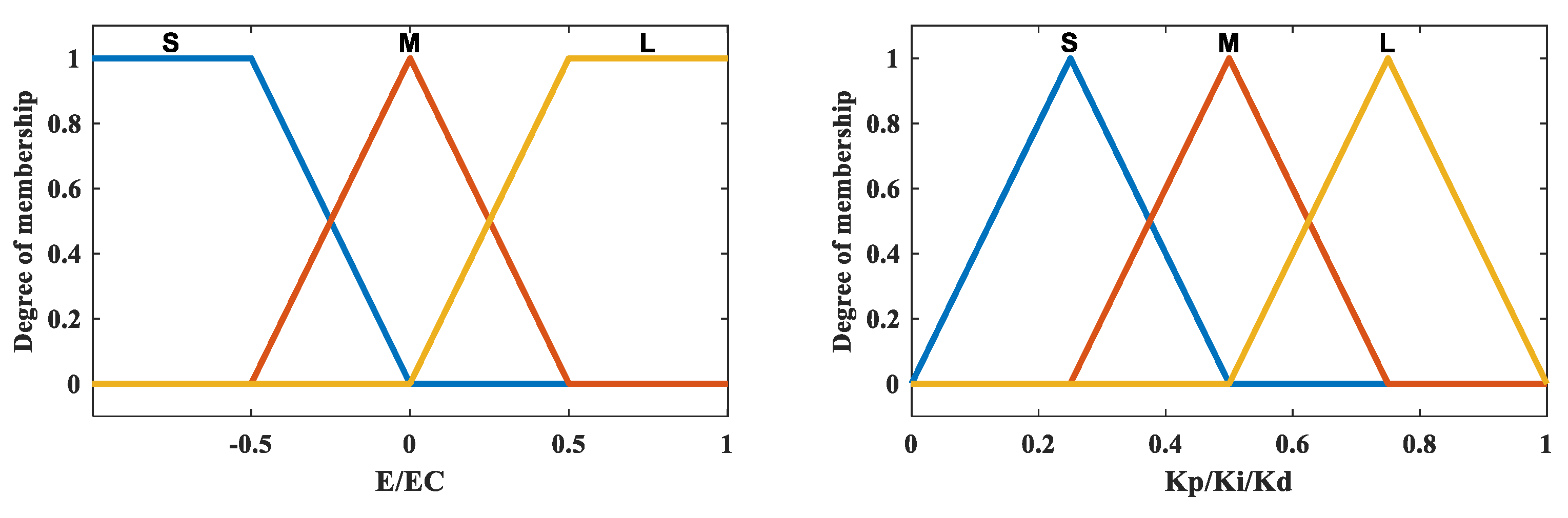
In the study, a total of three fuzzy inference systems were employed to choose the most effective one. The membership functions of the input and output fuzzy subsets were simply selected, shown in Figure 3, Figure 4 and Figure 5.

Fuzzy inference rules are depicted in

Table 1. Fuzzy rules for tuning PID gains (three fuzzy subsets).

Kp/Ki/Kd	E
		S	M	L
EC	S	M/S/S	M/S/S	L/S/S
	M	L/M/M	M/M/S	M/M/S
	L	L/L/L	M/L/S	S/L/S

,

Table 2. Fuzzy rules for tuning PID gains (four fuzzy subsets).

Kp/Ki/Kd		E
		L	M	S	ZO
EC	L	M/ZO/S	S/S/M	M/M/ZO	M/L/ZO
	M	L/ZO/M	M/S/M	L/L/S	L/L/ZO
	S	L/ZO/L	M/Z/L	L/L/S	L/L/S
	ZO	L/ZO/L	M/Z/L	L/L/S	ZO/ZO/ZO

and

Table 3. Fuzzy rules for tuning PID gains (seven fuzzy subsets).

Kp/Ki/Kd		EC
		NB	NM	NS	ZO	PS	PM	PB
E	NB	PB/NB/PS	PB/NB/NS	PM/NM/NB	PS/NM/NB	PS/NS/NB	ZO/ZO/NM	ZO/ZO/PS
	NM	PB/NB/PS	PB/NB/NS	PM/NM/NB	PS/NS/NM	PS/NS/NM	ZO/ZO/NS	NS/ZO/ZO
	NS	PM/NB/ZO	PM/NM/NS	PM/NS/NM	PS/NS/NM	ZO/ZO/NS	NS/PS/NS	NS/PS/ZO
	ZO	PM/NM/ZO	PM/NM/NS	PS/NS/NS	ZO/ZO/NS	NS/PS/NS	NM/PM/NS	NM/PM/ZO
	PS	PS/NM/ZO	PS/NS/ZO	ZO/ZO/ZO	NS/PS/ZO	NS/PS/ZO	NM/PM/ZO	NM/PB/ZO
	PM	PS/ZO/PB	ZO/ZO/NS	NS/PS/PS	NM/PS/PS	NM/PM/PS	NM/PB/PS	NB/PB/PB
	PB	ZO/ZO/PB	ZO/ZO/PM	NM/PS/PM	NM/PM/PM	NM/PM/PS	NB/PB/PS	NB/PB/PB

. The three tables represent the fuzzy inference rules for the cases with three, four, and seven fuzzy subsets of the input and output variables, respectively. For example, 4 subsets for both deviation E and deviation changing rate EC result in totally 4 × 4 rules, each of which gives out the fuzzy subsets of P, I, and D gains with four possibilities, respectively.

3.2. Neural Network Design

By discretizing the basic PID a digital-form PID formulation can be obtained as:

$$u(\mathrm{k})=k_{p}e(k)+k_i{\displaystyle {\sum }_{j=0}^{k}e(k)}+k_d[e(k)-e(k-1)]$$

(8)

then an incremental PID formulation can be described according to last three errors:

$$\Delta u(\mathrm{k})=k_p[e(k)-e(k-1)]+k_{i}e(k)+k_d[e(k)-2e(k-1)+e(k-2)]$$

(9)

$$u(\mathrm{k})=u(k-1)+\Delta u(k)$$

(10)

A two-layer feedforward neural network was constructed to generate the tuning vector for the original coefficients. The reference value for the OER, its actual output value, and the error between them, adding the constant input 1 which represents the offset, make up the total of four nodes for the input layer. The number of hidden layer nodes is set to seven appropriately, and certainly the output layer nodes are three so as to obtain three coefficients for PID gains. Figure 6 briefly displays the structure of the neural network.

As respect to the transition/activation functions, choose “tansig” function:

$${\phi }_1(x)=\frac{e^x-e^{-x}}{e^x+e^{-x}}=\frac{1-e^{-2x}}{1+e^{-2x}}$$

(11)

for the hidden layer, and “logsig” function

$${\phi }_2(x)=\frac{e^x}{e^x+e^{-x}}=\frac{1}{1+e^{-2x}}$$

(12)

for the output layer.

The weights of any two nodes between neighboring layers are adjusted according to the error back propagation principle. The error function is described as:

$$E(k)=\frac{1}{2}{[r(k)-y(k)]}^2$$

(13)

where $r(k)$ and $y(k)$ are the reference value and actual real-time value of the oxygen excess ratio at k moments, respectively. According to the gradient method, the adjusting formula for the weight coefficient of each neuron in the output layer is:

$$\Delta w_{ki}=-\eta \frac{\partial E(k)}{\partial w_{ki}}=-\eta \frac{\partial E(k)}{\partial ne{t}_k}·\frac{\partial ne{t}_k}{\partial w_{ki}}=-\eta \frac{\partial E(k)}{\partial ne{t}_k}·o_i$$

(14)

where $\eta$ denotes the learning rate, $ne{t}_k$ means the total input of the k-th neuron in the output layer, and $o_i$ is the output of the i-th neuron in the hidden layer. Define the intermediate part of the Formula (14) as:

$${\delta }_k^{(3)}=-\frac{\partial E(k)}{\partial ne{t}_k}=e(k)\frac{\partial y(k)}{\partial \Delta u(k)}\frac{\partial \Delta u(k)}{\partial O_k(k)}{\phi }_2^{\prime }(ne{t}_k)$$

(15)

where $e(k)=r(k)-y(k)$, is the error of the controlled variable, $u(k)$ denotes the current controller output through the network tuning. In practice, due to the unknown $\frac{\partial y(k)}{\partial \Delta u(k)}$, as an approximation it is replaced by the sign function $\mathrm{sgn}[\frac{\partial y(k)}{\partial \Delta u(k)}]$ in practice. As $k_p$, $k_i$, $k_d$ are the elements of the network output vector $O(k)$, $\frac{\partial \Delta u(k)}{\partial O_k(k)}$ can be obtained according to Equation (9). Finally, add an inertial term that makes the search converge fast and globally minimal, and the weight adjustment formula becomes

$$\Delta w_{ki}(n)=\eta {\delta }_k^{(3)}{o}_i+\alpha \Delta w_{ki}(n-1)$$

(16)

where $\alpha$ denotes the inertia coefficient which is between 0 and 1, $\Delta w_{ki}(n-1)=w_{ki}(n-1)-w_{ki}(n-2)$ denotes the weight change at the previous moment.

Similarly, the adjusting method for the weights of the hidden layer neurons is:

$$\Delta w_{ij}(n)=\eta {\delta }_i^{(2)}{o}_j+\alpha \Delta w_{ij}(n-1)$$

(17)

$${\delta }_i^{(2)}={\phi }_1^{\prime }(ne{t}_i){\displaystyle \sum _{k=1}^3{\delta }_k^{(3)}}{w}_{ki}$$

(18)

4. Results and Discussion

Concerning a convoluted complicated nonlinear system, linearizing the PEMFC plant model for a PID configuration may be a tough errand and also unnecessary. There have been a number of empirical or experimental methods summed up to tune the three gains for PID controllers. In this study, two relatively satisfactory results of the conventional PID control were obtained after a few tests using several tuning methods for gains. Next, three fuzzy inference systems were employed to tune PID gains, respectively. Moreover, a back-propagation neural network was also tried to tune these coefficients.

Several parameters or settings are concerned in the fuzzy inference system and the neural network, respectively. The Mamdani fuzzy inference systems in the fuzzy logic toolbox of Matlab software were employed in this study, and the default settings in the interface for the inference methods were retained, except for choosing “sum” as the aggregation method. The membership functions can be conveniently generated in the fuzzy logic toolbox, while the scale factors for transformations between the domains of discourse need to be cautiously addressed.

The neural network was implemented through an s-function integrated into the Simulink model. Four input parameters for the s-function could be easily but cautiously changed in the Masking interface. In our study, the learning rate $\eta$ was set at 0.2, the inertia coefficient $\alpha$ was 0.05, the number of hidden layer nodes j was finally set at 7, and the sampling time was 0.01 s.

4.1. Constant OER Response Test

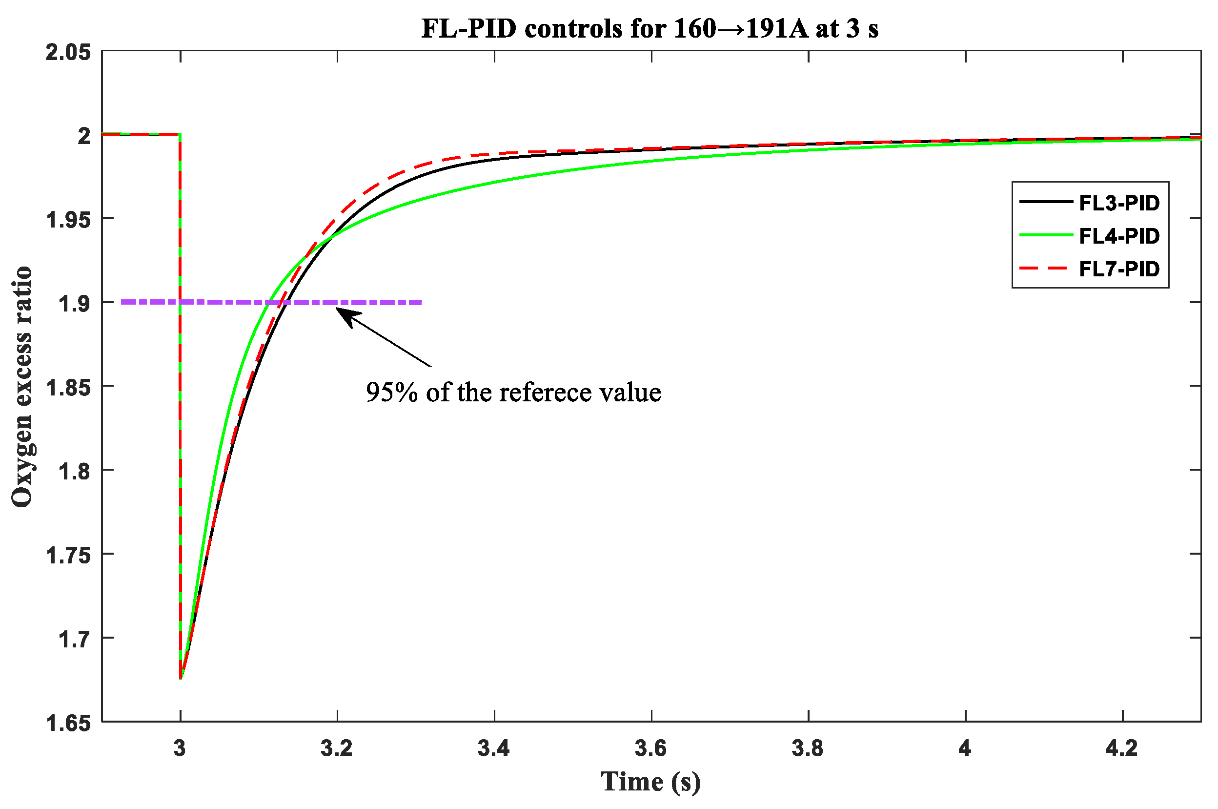
In the simulations, a constant setpoint value of 2 for the oxygen excess ratio was used first in a step response simulation, which allows the load current to change from 160 A to 191 A at 3 s. Figure 7 presents the OER responses with the PID gains tuned by three fuzzy inference systems, respectively, (corresponding control methods were named as FL3-PID, FL4-PID, and FL7-PID, respectively, according to the numbers of partitions of the respective fuzzy set). The purple line in the Figure 7 shows the 95% of the reference OER value, which eases the comparison of the settling times with these three controllers. Although the rising time of OER with FL4-PID is the shortest, the entire response is too sluggish with a settling time of about 1 s, which is obviously longer than 0.4–0.5 s in the other two cases. Comprehensively, the control methods using three subsets and seven subsets individually for the fuzzy set division behave better than the control using four subsets; furthermore, using seven subsets is a little faster than using three subsets to reach the final steady-state value.

In Figure 8, the constant oxygen excess ratio responses to the step load with four controls (named PID1, PID2, FL7-PID, and NN-PID, respectively) are displayed together. With PID2, the oxygen excess ratio increases more rapidly, yet an obvious overshoot instantly occurs unfavorably, which renders the final settling time of nearly 0.35 s; with PID 1, the rising curve becomes smooth without any overshoot or undershoot, and a settling time of about 0.32 s exhibits good performance. The FL7-PID (PID tuned by fuzzy logic inference with seven fuzzy subsets) can be recognized as the best, due to fast response speed (less than 0.1 s for the rising time, and 0.16 s for the settling time) with only a tiny overshoot, although the steady-state value of oxygen excess ratio needs more than 1 s to fully reach the setpoint value 2 (this situation can be improved by increasing the quantification factor of I part).

Distinctively, the neural network tuned PID controls behave differently in every simulation test, without changing any parameter, as the initial weights between neural network nodes are generated by random function and thus changeable each time. In Figure 8, three test results of the identical NN-PID control are shown, among which NN-PID-2 may be considered the best on the whole. Although these NN-PID tests show no advantage here, the NN method still has the potential to be upgraded via integration with other algorithms; for example, an optimal method may be adopted for providing the initial weights. In addition, it should be pointed out that the neural network in Figure 8 adopts seven hidden layer nodes, which was also compared in our study with other cases using different numbers of hidden layer nodes.

If the amplitude of the step load increases, such as from 160 A to 220 A (see Figure 9), there is also a certain overshoot with the PID1 control. On the other hand, the fuzzy logic tuned PIDs still present smooth curves and can be deemed as the best compared with the conventional PID and NN-PID methods; adjusting the quantification factor of I part for the FL7-PID method to a bigger value could fast enough make the oxygen excess ratio get more adjacent to the constant setpoint value (see FL7-PID-1, FL7-PID-2, and FL7-PID-3, with gradually increasing I-part coefficients); for example, the FL7-PID-3 exhibits quite a short rising time and reaches the setpoint value within less than 0.2 s. For NN-PID control, still three test results are shown in Figure 9 (see NN-PID-1, NN-PID-2, and NN-PID-3), among which NN-PID-3 may be considered to exhibit close performance to PID1, except for a delay for settling time of approximately 0.5 s.

4.2. Variable OER Response Test

Figure 10a shows the optimal OERs when the load current changes. This curve was obtained from the data for steady states, nevertheless, could still be utilized here for providing a series of corresponding changeable setpoints of the OER when the load current changes. It can be observed that the curve-fitted polynomial can represent the OER change with the load current well in the range of less than 220 A except for the point of 200 A; thus, a series of step load working conditions can be defined in Figure 10b for variable OER simulation tests, in which different OER reference values are generated conveniently by the polynomial.

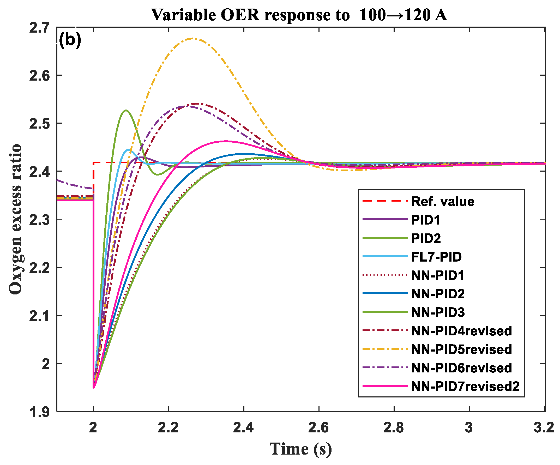
The simulation results for the variable control of the oxygen excess ratio are shown in Figure 11a. As to the first load current requests, the NN-PID control (three times of tests are showed) can reach the setpoint values with a smaller overshoot, but the settling time is approximately 1.2 s. It even gets worse that as the current increases, the settling times for the next two step load conditions become more and more longer (2 s and 2.5 s, respectively), although meanwhile overshoots gradually disappear. The FL7-PID fuzzy logic tuned PID method presents obvious advantages in the performance indices of both overshoots and settling time, and this could be observed clearly in the zoomed Figure 11b,c, which display the OER responses to the step load increases from 100 A to 120 A and from 160 A to 220 A, respectively. The settling times of FL7-PID concerned these two step loads are about 0.17 s and 0.25 s, respectively; for PID1 and PID2, the settling times are about 0.4–0.5 s and 0.45 s, respectively. Moreover, PID2 also exhibits considerably greater overshoots than PID1 and FL7-PID; the overshoot of PID1 on the condition of high load increases a little, while the overshoot of FL7-PID decreases clearly.

4.3. Discussion

4.3.1. About Fuzzy Logic Inference

The PID tuned with fuzzy logic, which used seven subsets for each fuzzy set, behaves satisfactorily under all the working conditions of the simulation tests, showing its advantage over the conventional PID and neural network controls. The distribution of fuzzy subsets and their membership functions can be further optimized to improve the control effect. Moreover, in the future, fuzzy inference system using formula method may be promising, which directly defines subsets of the input variables as fuzzy numbers and uses them to calculate the output fuzzy numbers through simple arithmetic operations. This method is such ingenious and convenient, but can be flexible by using a correction factor $b$ such as:

$$U=\langle bE+(1-b)EC\rangle ,b\in [0,1]$$

(19)

where $E$, $EC$, and $U$ are fuzzy numbers of the error, error change rate, and the output variable of the fuzzy inference system.

4.3.2. About Neural Network

As for the back propagation neural network, it still encounters two difficulties: one is the optimization issue for initial connection weights between neural network nodes, which may even lead to non-stable situations of the network if not generated properly by the random function; the other is that the OER responses with NN-PID to various load currents should be speeded up with less vibrations.

Another weight update method was also tried in our study. The updating algorithm is

$$w(k+1)=w(k)+\eta [(1-c)D(k)+cD(k-1)]$$

(20)

where $w(k+1)$, $w(k)$ are the weights at the adjacent moments, $D(k)$, $D(k-1)$ are the negative gradients of the performance index at the adjacent moments $D(k)=-\partial E/\partial w(k)$. c herein is called momentum factor and intelligibly its range is [0, 1].

Through updating the output layer weights with this method, the NN-PID could catch up to the OER demand more quickly than with the original weight update method when a step-up current of 60 A is required at 8 s (see the dash dot lines for NN-PID (4–6)-revised in Figure 12a); however, it is still regrettable that the settling times are still longer than other methods mentioned in this paper. Moreover, when a greater increase of oxygen excess ratio from 2.34 to 2.42 is requested, corresponding to a current change from 100 A to 120 A, large overshoots may occur (see Figure 12b). Therefore, how to realize the general consideration becomes a problem.

Next, we tried using changeable learning rates for updating weights of the output layer. $\eta$ in Equation (20) is replaced by the following formula:

$$\eta (k)=x^{\lambda }\eta (k-1)$$

(21)

$$\lambda =\mathrm{sgn}[D(k)D(k-1)]$$

(22)

where $\eta (k)$ and $\eta (k-1)$ represent the learning rates of two adjacent steps, $x$ denotes a real number between 1 and 2 (finally x = 1.4 was chosen), $\lambda$ is determined by the gradient direction of two successive generations. When the gradient direction of two successive generations is the same, it indicates that the descent speed is too slow, and the step size can be enlarged; when the gradient direction is opposite for two consecutive times, it indicates that the descending speed is too fast, and the step size can be shortened.

By adding this adjusting strategy for the learning rate to the weight update method (Equation (20)), a relatively better control NN-PID7revised2 is obtained (see Figure 12a,b), with which the requirements of rapidity of high current section and small overshoot of low current section are balanced, to an extent. With NN-PID7revised2 control, the overshoot of oxygen excess ratio is observably reduced during the current step-up from 100 A to 120 A compared with those by the NN-PID (4–6)-revised control; meanwhile, close performance to NN-PID4revised and NN-PID6revised is obtained during the third step-up working condition.

The simulation results of the above constant OER response test with the change in load current of “160→191 A” (see Figure 8) and the section “100→120 A” in the variable OER response test (see Figure 12b) for the change in load current of “100→120→160→220 A” can be summarized in

Table 4. Control results of OER regulation or tracking with four control methods.

Operation Condition	Control Method	Overshoot (%)	Peak Time (s)	Settling Time (s)
Constant OER response to 160→191 A	PID1	0.11	0.231	0.32
	PID2	2.55	0.116	0.35
	FL7-PID	0.42	0.108	0.16
	NN-PID2	1.13	0.391	0.84
Variable OER response to 100→120 A	PID1	0.85	0.125	0.23
	PID2	4.47	0.085	0.24
	FL7-PID	1.09	0.090	0.18
	NN-PID7revised2	2.25	0.346	0.68

for comparison. Therefore, it is obviously observed that the fuzzy PID controller with seven subsets acquires the best dynamic performance in both constant OER regulation and variable OER tracking.

4.3.3. About Fractional Order PID

When dealing with nonlinear controlled plants, using fractional order PID may acquire better control efficacy than using conventional PID; thus, we tried using fractional order PID controllers based on PID2 and FL7-PID, respectively. The orders for integral and derivative terms of the controller were finally selected at 1.15 and 1.3, respectively, through several simulation comparisons based on the original PID2.

The response comparisons of the four controllers for variable OER under the load conditions in Figure 10b are displayed in Figure 13. It can be observed that the fractional order PID (FOPID2) can reduce the overshoots of the OER and even eliminate the undershoots in the transient processes. The fuzzy fractional order PID (FL7-FOPID) also exhibited smaller overshoots than FL7-PID, but there were also two defects with FL7-FOPID: one is that when the OER needed to increase for the current request 100→120 A, a time delay of more than 1.2 s existed after the previous rapid rising process, which rendered the final settling time more than 1.5 s; the other is that the steady-state error of OER with FL7-FOPID was a little bigger than with the other methods. By increasing the quantification factor of part I, the first defect could be greatly improved (see FL7-FOPID-r1 in Figure 13c, shortened settling times in all transients); however, the steady-state error remains an issue. Therefore, so far in our study, the FL7-PID controller is still the proposed one.

5. Conclusions

For improving the oxygen supply for a PFMFC system, intelligent techniques including three fuzzy logic inference systems and a neural network were employed to adjust the gain coefficients of PID controllers. Simulation results demonstrate that the PID controller integrated with the fuzzy logic inference with seven subsets (FL7-PID) has the best control efficacy in both constant-value OER response tests and variable OER response tests, with small overshoots and the fastest settling times of less than 0.2 s, exhibiting obvious advantages over conventional PID methods.

On the other hand, the neural network tuned PID could render control effect approximate to conventional PIDs when dealing with constant OER regulations, except for the delay of settling times of about 0.5 s. However, its responses to variable OER requests are too sluggish (more than 1 s for the settling times). Through adding a momentum term and adopting changeable learning rates for the weight update of the output layer, improved performance (for example, less than 0.7 s for the settling time) is achieved to an extent. In addition, fractional order PID controllers can also render smaller overshoots than conventional PID controllers in the simulation of variable OER response tests.

In the future, other methods may be integrated to further improve the NN-PID method; for example, an optimization algorithm will be of benefit to obtaining the proper initial weights for the neural network nodes, or directly, optimization based intelligent tuning methods for PID can be considered. On the other hand, there are numerous other attractive realization forms for a fuzzy inference system, which may be applied to achieve good results in fuel cell control. Moreover, a state observer for the cathode pressure could also be considered in view of the difficulty for obtaining accurate measurement.