Enhancing Power Grid Resilience through Real-Time Fault Detection and Remediation Using Advanced Hybrid Machine Learning Models

Abstract

Ensuring a reliable and uninterrupted supply of electricity is crucial for sustaining modern and advanced societies. Traditionally, power systems analysis was mostly dependent on formal commercial software, mathematical models produced via a mix of data analysis, control theory, and statistical methods. As power grids continue to grow and the need for more efficient and sustainable energy systems arises, attention has shifted towards incorporating artificial intelligence (AI) into traditional power grid systems, making their upgrade imperative. AI-based prediction and forecasting techniques are now being utilized to improve power production, transmission, and distribution to industrial and residential consumers. This paradigm shift is driven by the development of new methods and technologies. These technologies enable faster and more accurate fault prediction and detection, leading to quicker and more effective fault removal. Therefore, incorporating AI in modern power grids is critical for ensuring their resilience, efficiency, and sustainability, ultimately contributing to a cleaner and greener energy future. This paper focuses on integrating artificial intelligence (AI) in modern power generation grids, particularly in the fourth industrial revolution (4IR) context. With the increasing complexity and demand for more efficient and reliable power systems, AI has emerged as a possible approach to solve these difficulties. For this purpose, real-time data are collected from the user side, and internal and external grid faults occurred during a time period of three years. Specifically, this research delves into using state-of-the-art machine learning hybrid models at end-user locations for fault prediction and detection in electricity grids. In this study, hybrid models with convolution neural networks (CNN) have been developed, such as CNN-RNN, CNN-GRU, and CNN-LSTM. These approaches are used to explore how these models can automatically identify and diagnose faults in real-time, leading to faster and more effective fault detection and removal with minimum losses. By leveraging AI technology, modern power grids can become more resilient, efficient, and sustainable, ultimately contributing to a cleaner and greener energy future.

1. Introduction

The fourth energy revolution is witnessing the increasing integration of artificial intelligence in every industrial field across the globe. The energy production sector is no exception, and AI techniques are now playing a vital role in the process. As a result, power generation grid stations worldwide are quickly transitioning towards smart grids, which are the fundamental requirement for the near future. This shift is largely driven by the declining dependence on fossil fuels, which is happening progressively every day. Renewable energy resources such as solar, wind, hydel, biogas, and tidal power are taking center stage in the energy production arena and are rapidly replacing fossil fuels. However, developing and underdeveloped countries still face significant challenges in maintaining their power-generation grids, mainly due to the continued use of conventional tools and software. Therefore, there is a need to invest in modern technologies to support the transition towards renewable energy and the maintenance of power-generation grids in these countries. The detection, collection, and management of faults are critical components in ensuring the efficiency and dependability of intricate systems, such as industrial machinery, power grids, and transportation systems. However, these systems are susceptible to diverse kinds of faults and malfunctions, which can lead to expensive downtime, decreased productivity, and potentially dangerous safety risks [1,2,3,4,5,6,7]. Additionally, refs. [8,9,10] propose an autonomous load restoration architecture that enhances the resilience of power distribution grids against HILP events. The solution is resilience-driven, uses imported power, distributed energy resources, and vehicle-to-grid capacity, and includes a resilience evaluation framework. Real-world testing demonstrates the efficacy of the proposed solution in enhancing the resilience of power-distribution systems against HILP scenarios. Traditional fault detection and management methods rely on rule-based expert systems designed to detect specific types of faults based on predetermined criteria [11,12,13,14,15,16]. However, these methods are limited in their ability to adapt to new and unpredictable fault patterns and require a significant amount of domain expertise to develop and maintain [15]. Currently, there has been a growing interest in using artificial intelligence (AI) and machine learning techniques for fault detection and management [16]. Machine learning in AI offers a promising approach for automating the process of fault detection and management by enabling systems to learn from data and adapt to new and changing fault patterns [17]. This research article aims to review the current state-of-the-art application of AI and machine learning techniques for fault detection, collection, and management in complex systems [18]. In recent years, there has been a substantial rise in interest in using AI strategies for fault detection. One of the main advantages of these techniques is their ability to identify and classify faults based on data patterns without the need for explicit rule-based systems [19]. Several machine learning algorithms have been proposed for fault detection, including deep neural networks (DNN), support vector machines (SVM), decision trees (DT), and Bayesian networks (BN) [20]. These algorithms may be taught to learn patterns and correlations between multiple variables by being trained on historical data. These patterns and relationships can reveal the existence of problems in the system. Once trained, these algorithms can be used to classify new data and identify the presence of faults in real-time [21]. In addition to fault detection, these machine learning models can also be used for fault collection and management. Regarding this issue, previous research has been conducted [22] in which fault collection involves the process of gathering and analyzing data related to faults in the system. These data can be used to identify the root cause of faults and develop strategies for preventing similar faults in the future [23]. Machine learning algorithms can be used to analyze large datasets of fault data to identify patterns and relationships between different variables that can be used to develop predictive models for fault management [24]. These predictive models can identify potential faults before they occur and develop proactive maintenance strategies to prevent downtime and reduce costs [25]. Machine learning fault detection and management models are a rapidly growing field with many applications in various industries. However, several challenges need to be addressed to ensure the effectiveness and reliability of these techniques. One of the main challenges is the availability of high-quality data for training and testing machine learning algorithms [26]. Another challenge is the interpretability of machine learning models, as many models operate as “black boxes”, and it can be challenging to understand how they make decisions [27]. Additionally, there are concerns about the ethical implications of using AI machine learning for fault detection and management, particularly in safety-critical systems [28]. The use of ML in power systems has been widely explored in the literature [29]. Various machine learning models such as artificial neural networks (ANNs), decision trees (DTs), support vector machines (SVMs), and hybrid and ensemble methods have been applied for fault detection, prediction, and removal. Among these techniques, hybrid models have gained increasing attention due to their ability to combine the strengths of different models to achieve better performance. One of the most popular types of hybrid models is the combination of convolutional neural networks (CNNs) and recurrent neural networks (RNNs), including long short-term memory (LSTM) and gated recurrent units (GRUs) [30]. CNNs are used to extract the spatial features of fault signals, while RNNs are utilized to capture the temporal dependencies. CNN-RNN hybrid models have been applied to fault diagnosis in power systems [31] and have shown promising results. Another type of hybrid model that has been applied to fault detection in power systems is the combination of CNNs and gradient boosting methods such as XGBoost and AdaBoost. Several strategies have been used to make the categorization more accurate while lowering false alarms [32]. Support vector machines (SVMs) have also been applied as a hybrid model with CNNs for fault detection [33]. The combination of SVM and CNN can improve detection accuracy by reducing the noise in the data. Furthermore, ensemble methods such as random forests have also been applied in hybrid models for fault detection and diagnosis [34]. Ensemble methods are known for reducing overfitting and improving models’ generalization performance [35]. For instance, in [36], a hybrid model combining a deep belief network and a self-organizing map was proposed for fault diagnosis in power systems. Another study [37] proposed a hybrid model that combines a stacked denoising autoencoder and a deep neural network for fault detection and classification. A hybrid model combining wavelet transform, PCA, and a back propagation neural network was proposed in [38] for power transformer fault diagnosis. Other studies have explored the use of hybrid models in other aspects of power systems, such as load forecasting and energy management. For instance, a hybrid model combining a deep learning model and an ARIMA model was proposed in [39] for short-term load forecasting. Another study [40] proposed a hybrid model that combines clustering and reinforcement learning for energy management in microgrids. Overall, the application of hybrid machine learning models in power systems has shown promising results, and further research in this area can lead to more effective and reliable power systems.

In this research, AI techniques, specifically hybrid machine learning models, are integrated for real-time fault prediction and detection in modern power generation grids. The goal is to enhance the resilience, efficiency, and sustainability of power grids by leveraging AI technology for faster and more effective fault removal. This aligns with the objective of achieving a cleaner and greener energy future in the context of the fourth industrial revolution (4IR). Additionally, feature selection techniques are investigated to improve the efficiency of the proposed approach. The following novelties are present in this research work:

• Utilization of real-time fault collection data from a working power grid station situated in Saudi Arabia, which is a significant contribution to the research. The rarity of faults in the station made the data collection process time-consuming, making it a valuable addition to the literature.
• Implementation of artificial intelligence techniques in this research for a power grid station, which is a unique idea and has not been implemented before. This innovation challenges the traditional software currently in use in most grid stations.
• Acknowledgment of the need for further improvement in this research area and the intention to explore similar ideas.

The rest of the paper is structured as follows: Section 2 describes the process of fault detection, prediction, and removal in power systems using hybrid machine-learning models. Additionally, the structure of models, along with mathematical equations, has been discussed. Section 3 explains the case study in which the description of data is given, i.e., from where and how data are collected. Section 4 presents a performance evaluation, graphical visualizations, and experimental results for the proposed approach. Finally, Section 5 concludes the paper.

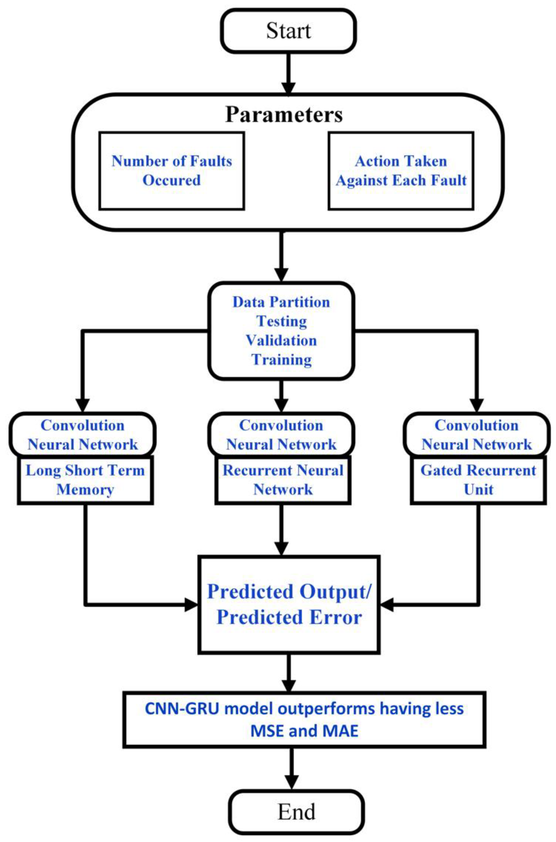
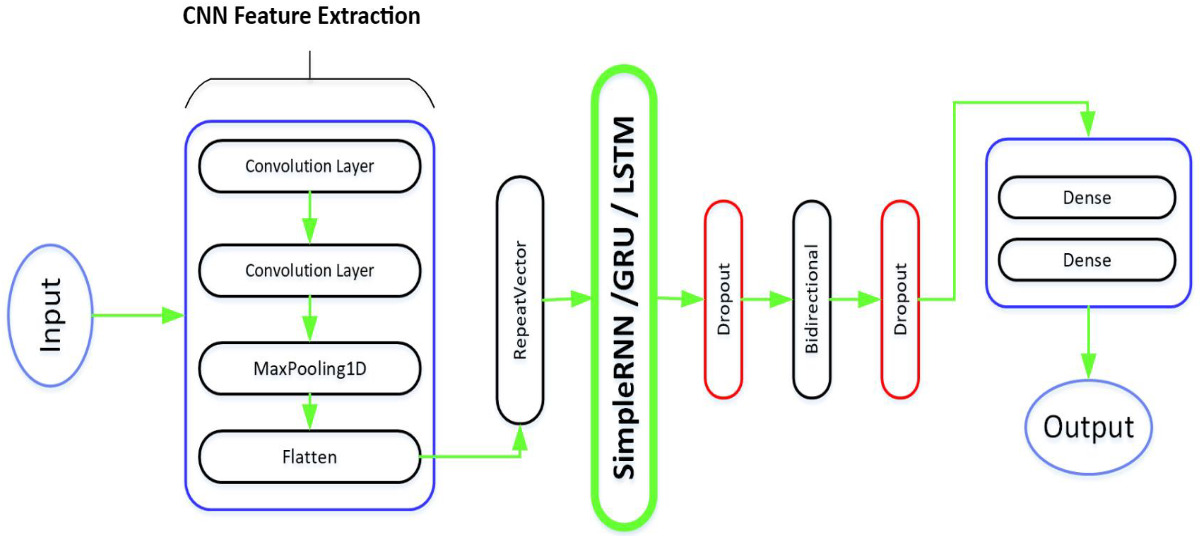
2. Proposed Framework for Fault Prediction and Elimination

Figure 1 illustrates that the hybrid model framework that has been developed makes use of four factors, including regular users, VIP users, faults that happened, and the action that is taken in response to those problems. For the goal of prediction, three different hybrid models, namely, CNN-RNN, CNN-GRU, and CNN-LSTM, are chosen and trained using 70% of the real-time data collected by the grid station, while the remaining 30% of the data are set aside for the purposes of validation and testing. The outcomes of the prediction are graphically represented, and after making a comparison between the two representations, it is clear that the CNN-GRU model performs better than the other two hybrid models. Additionally, the mean error values that are generated by the CNN-GRU model are noticeably lower than those that are generated by other hybrid models.

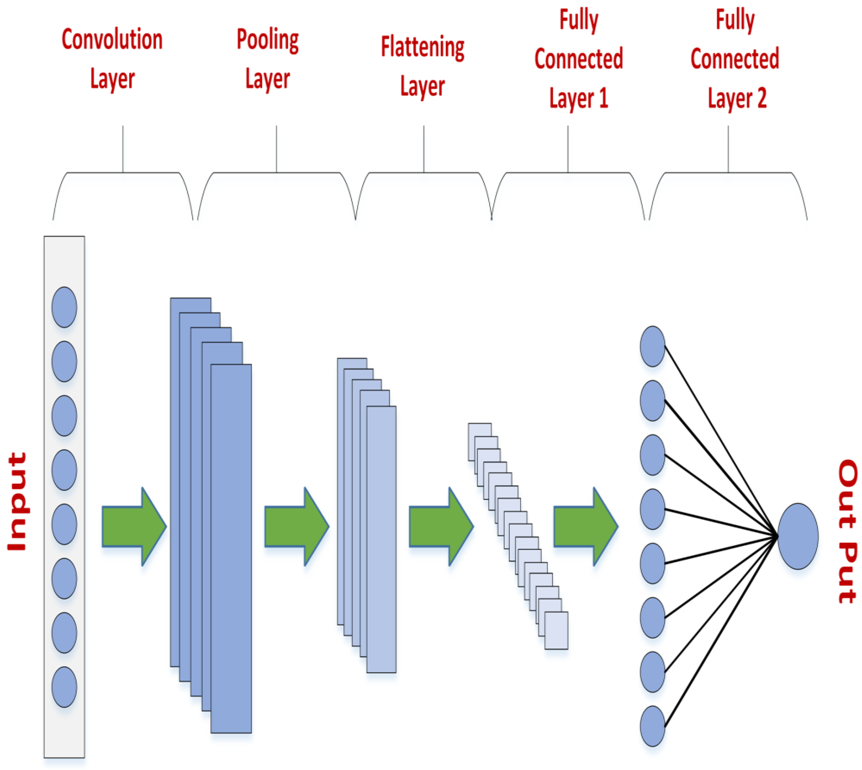
2.1. Structure of Convolutional Neural Network

Convolutional Neural Networks, often known as CNNs, are a specific sort of neural network design that has been shown to be helpful in time series analysis. This is particularly true in the context of tasks such as signal processing, voice recognition, and picture analysis. The core idea behind CNNs is that they use layers, which are small matrices of weights convolved with the input data. For example, in the context of time series analysis, the input data could be a sequence of time-stamped data points, and the layers could be designed to extract relevant features from this sequence. The structure of a CNN is shown in Figure 2.

The main layers and their functionality in this process are discussed as follows:

2.1.1. Convolution Layer

The input sequence is convolved with a set of layers to produce a set of feature outputs. Each output is obtained by sliding the layer along the input sequence and calculating the dot product that exists between the layer and the input subsequence that corresponds to it.

2.1.2. Non-Linearity

A non-linear activation function is applied to each element of the layer outputs. This step introduces non-linearities into the model, which enables it to learn complex patterns in the data.

2.1.3. Pooling Layer

The layer outputs are down-sampled by applying a pooling function, such as max pooling or average pooling, which reduces the spatial dimensions of the layer outputs while preserving their salient features.

2.1.4. Dropout

A regularization technique called dropout can be applied to the output of the pooling layer to prevent overfitting. Dropout randomly sets a fraction of the activations to zero during training, which forces the model to learn more robust features.

2.1.5. Fully Connected Layer

The output of the convolutional layers is first transformed into a vector and then fed into one or more fully connected layers. These layers are responsible for the classification or regression job at the end.

2.2. Structure of RNN, GRU, and LSTM

2.2.1. Recurrent Neural Networks (RNNs)

RNNs can process time-series data and sequential data. The RNN cell structure consists of a series of “memory cells” that can maintain information over time, as shown in Figure 3a. Each memory cell is connected to the next memory cell in the sequence, forming a chain-like structure. At each time step, the input is fed into the first memory cell, which updates its internal state and passes the information to the next memory cell. The output of each memory cell is a function of its internal state and the input at that time step. The critical difference between RNNs and other neural network architectures is that the output of a memory cell at each time step is also fed back into the next memory cell in the sequence. This allows the network to maintain a “memory” of previous inputs and use it to predict future inputs. Equations (1) and (2) show the mathematical expression for the internal structure of the Recurrent Neural Network Unit [22]:

$${\mathrm{H}}_{\mathrm{t}-1}=\mathsf{\sigma } ({\mathrm{P}}_{\mathrm{h}}\ast {\mathrm{H}}_{\mathrm{t}-1}+{\mathrm{P}}_{\mathrm{x}}\ast {\mathrm{X}}_{\mathrm{t}}+{\mathrm{B}}_{\mathrm{a}})$$

(1)

$${\mathrm{Y}}_{\mathrm{t}}=\mathrm{t}\mathrm{a}\mathrm{n}\mathrm{h} ({\mathrm{P}}_{\mathrm{o}}\ast {\mathrm{H}}_{\mathrm{t}}+{\mathrm{B}}_{\mathrm{o}})$$

(2)

where:

• ${\mathrm{H}}_{\mathrm{t}-1}$: The “hidden state” at time t – 1, which is a vector that summarizes the previous input sequence up to time t – 1. It is computed as the output of a sigmoid activation function (σ) applied to the weighted sum of the previous hidden state ${\mathrm{P}}_{\mathrm{h}}$ ∗ ${\mathrm{H}}_{\mathrm{t}-1}$ and the current input ${\mathrm{P}}_{\mathrm{x}}\ast {\mathrm{X}}_{\mathrm{t}}$ plus a bias term ${\mathrm{B}}_{\mathrm{a}}$.
• ${\mathrm{X}}_{\mathrm{t}}$: The input to the SRNN at time t.
• ${\mathrm{Y}}_{\mathrm{t}}$: The output of the SRNN at time t, which is a transformed version of the hidden state ${\mathrm{H}}_{\mathrm{t}}$ computed using a hyperbolic tangent activation function (tanh), and a weight matrix ${\mathrm{P}}_{\mathrm{o}}$ plus a bias term ${\mathrm{B}}_{\mathrm{o}}$.
• ${\mathrm{P}}_{\mathrm{h}}$: The weight matrix that determines the influence of the previous hidden state on the current hidden state.
• ${\mathrm{P}}_{\mathrm{x}}$: The weight matrix that determines the influence of the current input on the current hidden state.
• ${\mathrm{B}}_{\mathrm{a}}$: The bias term that determines the baseline activation level of the hidden state.
• ${\mathrm{P}}_{\mathrm{o}}$: The weight matrix that determines how the hidden state is transformed into the output.
• ${\mathrm{B}}_{\mathrm{o}}$: The bias term that determines the baseline activation level of the output.

Overall, the RNN equation represents that it uses the previous hidden state and current input state to compute the current hidden state, which is further used to compute the output at the current time step.

Figure 3. Basic structure of (a) RNN; (b) GRU; (c) LSTM.

Figure 3. Basic structure of (a) RNN; (b) GRU; (c) LSTM.

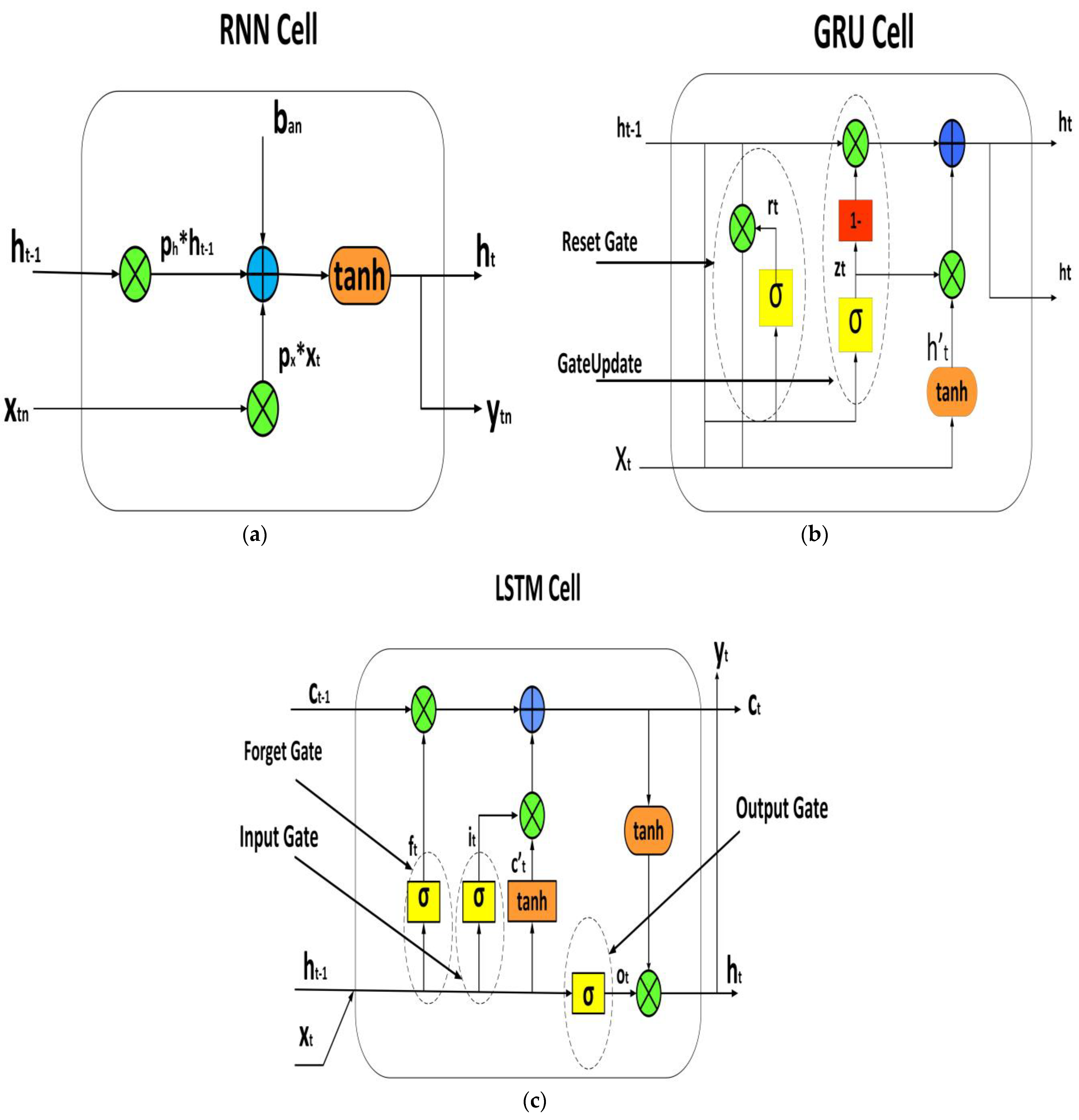
2.2.2. Gated Recurrent Units

GRUs are a particular kind of recurrent neural network that was developed as an alternative to long short-term memory (LSTM). Figure 3b illustrates the internal structure, which is comparable to that of an LSTM but has fewer parameters. Much like an LSTM, a GRU comprises a group of memory cells that can retain information over a period of time; however, in contrast to an LSTM, a GRU utilizes a gating mechanism to govern the flow of information between its memory cells. Two gates make up a GRU; the first gate is known as the reset gate, and the second gate is known as the update gate. The update gate is positioned to decide how much of the last memory should be kept and how much new state should be built up from the current input. The reset gate determines the amount of the initial memory state that will be forgotten. Before computing the update and reset gates, the input at each time step is first put through a series of linear transformations. These transformations are what are utilized to determine the state of the gates. After that, the update gate and the reset gate are put to use in order to update the state of the present memory cell, which is a mix of the state it was in before and the input it is receiving at the moment. The ultimate output of the GRU is a function of the state of the memory cell at each time step, and this output may be put to use for tasks involving either prediction or classification. The mathematical expression describing the internal structure of the Gate Recurrent Unit can be found in Equations (3)–(6), which read as follows [22]:

$${\mathrm{R}}_{\mathrm{t}}=\mathsf{\sigma } ({\mathrm{W}}_{\mathrm{r}\mathrm{h}}\ast {\mathrm{H}}_{\mathrm{t}-1}+{\mathrm{W}}_{\mathrm{r}\mathrm{x}}\ast {\mathrm{X}}_{\mathrm{t}})$$

(3)

$${\mathrm{Z}}_{\mathrm{t}}=\mathsf{\sigma } ({\mathrm{W}}_{\mathrm{z}\mathrm{h}}\ast {\mathrm{H}}_{\mathrm{t}-1}+{\mathrm{W}}_{\mathrm{z}\mathrm{x}}\ast {\mathrm{X}}_{\mathrm{t}})$$

(4)

$${{\mathrm{H}}^{\prime }}_{\mathrm{t}}=\mathrm{t}\mathrm{a}\mathrm{n}\mathrm{h} \{{\mathrm{W}}_{{\mathrm{h}}^{\prime }\mathrm{h}}\ast \left({\mathrm{R}}_{\mathrm{t}}\ast {\mathrm{H}}_{\mathrm{t}-1}\right)+{\mathrm{W}}_{{\mathrm{h}}^{\prime }\mathrm{x}}\ast {\mathrm{X}}_{\mathrm{t}}\}$$

(5)

$${\mathrm{H}}_{\mathrm{t}}=\{\left(1-{\mathrm{Z}}_{\mathrm{t}}\right){\mathrm{H}}_{\mathrm{t}-1}+{\mathrm{Z}}_{\mathrm{t}}\ast {{\mathrm{H}}^{\prime }}_{\mathrm{t}}\}$$

(6)

where:

• ${\mathrm{R}}_{\mathrm{t}}$: The “reset gate” controls how much of the previous hidden state ${\mathrm{H}}_{\mathrm{t}-1}$ is retained and how much is reset based on the current input ${\mathrm{X}}_{\mathrm{t}}$. It is computed as the element-wise multiplication of the output of a sigmoid activation function (σ) applied to the weighted sum of the previous hidden state ${\mathrm{W}}_{\mathrm{r}\mathrm{h}}\ast {\mathrm{H}}_{\mathrm{t}-1}$ and the current input ${\mathrm{W}}_{\mathrm{r}\mathrm{x}}\ast {\mathrm{X}}_{\mathrm{t}}$.
• ${\mathrm{Z}}_{\mathrm{t}}$: The “update gate” determines how much of the previous hidden state ${\mathrm{H}}_{\mathrm{t}-1}$ should be updated with the new candidate hidden state H′(t). It is computed as the output of a sigmoid activation function (σ) applied to the weighted sum of the previous hidden state (${\mathrm{W}}_{\mathrm{z}\mathrm{h}}\ast {\mathrm{H}}_{\mathrm{t}-1}$) and the current input (${\mathrm{W}}_{{\mathrm{h}}^{\prime }\mathrm{x}}\ast {\mathrm{X}}_{\mathrm{t}}$).
• ${{\mathrm{H}}^{\prime }}_{\mathrm{t}}$: The “candidate hidden state” represents a new candidate for the next hidden state based on the current input ${\mathrm{X}}_{\mathrm{t}}$ and the previous hidden state ${\mathrm{H}}_{\mathrm{t}-1}$ modified by the reset gate. It is computed as the output of a hyperbolic tangent activation function (tanh) applied to the weighted sum of the reset gate ${\mathrm{R}}_{\mathrm{t}}$ and the previous hidden state ${\mathrm{W}}_{{\mathrm{h}}^{\prime }\mathrm{h}}\ast \left({\mathrm{R}}_{\mathrm{t}}\ast {\mathrm{H}}_{\mathrm{t}-1}\right)$ and the current input ${\mathrm{W}}_{{\mathrm{h}}^{\prime }\mathrm{x}}\ast {\mathrm{X}}_{\mathrm{t}}$.
• ${\mathrm{H}}_{\mathrm{t}}$: The “hidden state” represents the output of the LSTM cell at time t, which is a combination of the previous hidden state ${\mathrm{H}}_{\mathrm{t}-1}$ and the new candidate hidden state ${{\mathrm{H}}^{\prime }}_{\mathrm{t}}$ based on the update gate. It is computed as a weighted sum of the previous hidden state ($1-{\mathrm{Z}}_{\mathrm{t}}$) and the new candidate hidden state (${\mathrm{Z}}_{\mathrm{t}}\ast {{\mathrm{H}}^{\prime }}_{\mathrm{t}}$).
• ${\mathrm{X}}_{\mathrm{t}}$: The input to the LSTM cell at time t.
• ${\mathrm{H}}_{\mathrm{t}-1}$: The previous hidden state of the LSTM cell at time t − 1.

2.2.3. Long Short-Term Memory (LSTM)

The internal structure of LSTM, which is likewise a sort of recurrent neural network RNN, can be seen in Figure 3c. Long-term dependencies in sequential data can be captured, and the vanishing gradient issue can be solved. The internal structure of an LSTM consists of a series of memory cells, each with a set of gates that control the flow of information through the cell. It consists of three types of gates: input, output, and forget gate. At each time step, the input is first passed through a set of linear transformations, which are used to compute the activations of the gates. The forget gate determines which information to discard from the previous memory state, the input gate determines which new information to add to the current memory state, and the output gate determines which information to output from the current memory state. The internal state of an LSTM cell is updated using a combination of the previous state and the new information, which is controlled by the forget and input gates. The output gate then determines which information to pass on to the next cell in the sequence. LSTMs effectively handle long-term dependencies in various sequential data tasks, including natural language processing, time-series prediction, and speech recognition. The mathematical expressions for the internal structure of the Long Short Term Memory Unit in Equations (7)–(12) are as follows [22]:

$${\mathrm{F}}_{\mathrm{t}}=\mathsf{\sigma } \left\{{\mathrm{W}}_{\mathrm{F}}\right({\mathrm{H}}_{\mathrm{t}-1},{\mathrm{X}}_{\mathrm{t}}\left)\right\}$$

(7)

$${\mathrm{I}}_{\mathrm{t}}=\mathsf{\sigma } \left\{{\mathrm{W}}_{\mathrm{I}}\right({\mathrm{H}}_{\mathrm{t}-1},{\mathrm{X}}_{\mathrm{t}}\left)\right\}$$

(8)

$${{\mathrm{C}}^{\prime }}_{\mathrm{t}}=\mathrm{t}\mathrm{a}\mathrm{n}\mathrm{h} \{{\mathrm{W}}_{\mathrm{C}}\ast \left({\mathrm{H}}_{\mathrm{t}-1},{\mathrm{X}}_{\mathrm{t}}\right)$$

(9)

$${\mathrm{C}}_{\mathrm{t}}=\left({\mathrm{F}}_{\mathrm{t}}\ast {\mathrm{C}}_{\mathrm{t}-1}\right)+{\mathrm{C}}_{\mathrm{t}}\ast {{\mathrm{C}}^{\prime }}_{\mathrm{t}}$$

(10)

$${\mathrm{O}}_{\mathrm{t}}=\mathsf{\sigma } \left\{{\mathrm{W}}_{\mathrm{O}}\right({\mathrm{H}}_{\mathrm{t}-1},{\mathrm{X}}_{\mathrm{t}}\left)\right\}$$

(11)

$${\mathrm{H}}_{\mathrm{t}}={\mathrm{O}}_{\mathrm{t}}\ast \tanh \left({\mathrm{C}}^{\mathrm{t}}\right)$$

(12)

where:

• ${\mathrm{H}}_{\mathrm{t}-1}$: The “hidden state” at time t − 1, which is a vector that summarizes the previous input sequence up to time t − 1.
• ${\mathrm{X}}_{\mathrm{t}}$: The input to the LSTM network at time t.
• ${\mathrm{F}}_{\mathrm{t}}$: The “forget gate” at time t, which determines how much of the previous cell state should be kept and how much should be forgotten. It is computed as the output of a sigmoid activation function (σ) applied to the weighted sum of the previous hidden state and the current input.
• ${\mathrm{I}}_{\mathrm{t}}$: The “input gate” at time t, which determines how much of the new input should be added to the cell state. It is computed as the output of a sigmoid activation function (σ) applied to the weighted sum of the previous hidden state and the current input.
• ${{\mathrm{C}}^{\prime }}_{\mathrm{t}}$: The “candidate cell state” at time t, which represents the candidate new values that could be added to the cell state. It is computed as the output of a hyperbolic tangent activation function (tanh) applied to the weighted sum of the previous hidden state and the current input.
• ${\mathrm{C}}_{\mathrm{t}}$: The “cell state” at time t, which represents the memory of the LSTM network at time t. It is computed as the combination of the previous cell state ${\mathrm{C}}_{\mathrm{t}-1}$ multiplied by the forget gate, ${\mathrm{F}}_{\mathrm{t}}$ and the current candidate cell state ${{\mathrm{C}}^{\prime }}_{\mathrm{t}}$ multiplied by the input gate, ${\mathrm{I}}_{\mathrm{t}}$.
• ${\mathrm{O}}_{\mathrm{t}}$: The “output gate” at time t, which determines how much of the cell state should be output as the hidden state. It is computed as the output of a sigmoid activation function (σ) applied to the weighted sum of the previous hidden state and the current input.
• tanh ${\mathrm{C}}_{\mathrm{t}}$: The hyperbolic tangent function applied to the cell state at time t.
• ${\mathrm{H}}_{\mathrm{t}}$: The “output” or “hidden state” at time t, which is the final output of the LSTM network at time t. It is computed as the element-wise multiplication of the output gate ${\mathrm{O}}_{\mathrm{t}}$ and the hyperbolic tangent of the cell state tanh ${\mathrm{C}}_{\mathrm{t}}$.
• ${\mathrm{W}}_{\mathrm{F}}$, ${\mathrm{W}}_{\mathrm{I}}$, ${\mathrm{W}}_{\mathrm{c}}$, and ${\mathrm{W}}_{\mathrm{o}}$: The weight matrices that determine how much each input and hidden state element affects the forget gate, input gate, candidate cell state, and output gate, respectively.

The next section, Section 3, details the case study in which the details about the collected data are given, which is further divided into Section 3.1 and Section 3.2, i.e., data collection and data analysis.

3. Case Study

To conduct this investigation, a grid station located in a particular area collected one-year real-time data from 2017 to 2022. The system’s distribution side employed physical and logical alarms to detect and gather information about any issues that may occur. The alerts were then categorized, and corrective or preventive measures were implemented accordingly. In this region, there are two types of energy consumers: VIP users, which are given priority, and normal users, which are charged at a standard rate. The system logs the event only when the defect has been resolved; otherwise, the problem is categorized as requiring further corrective action.

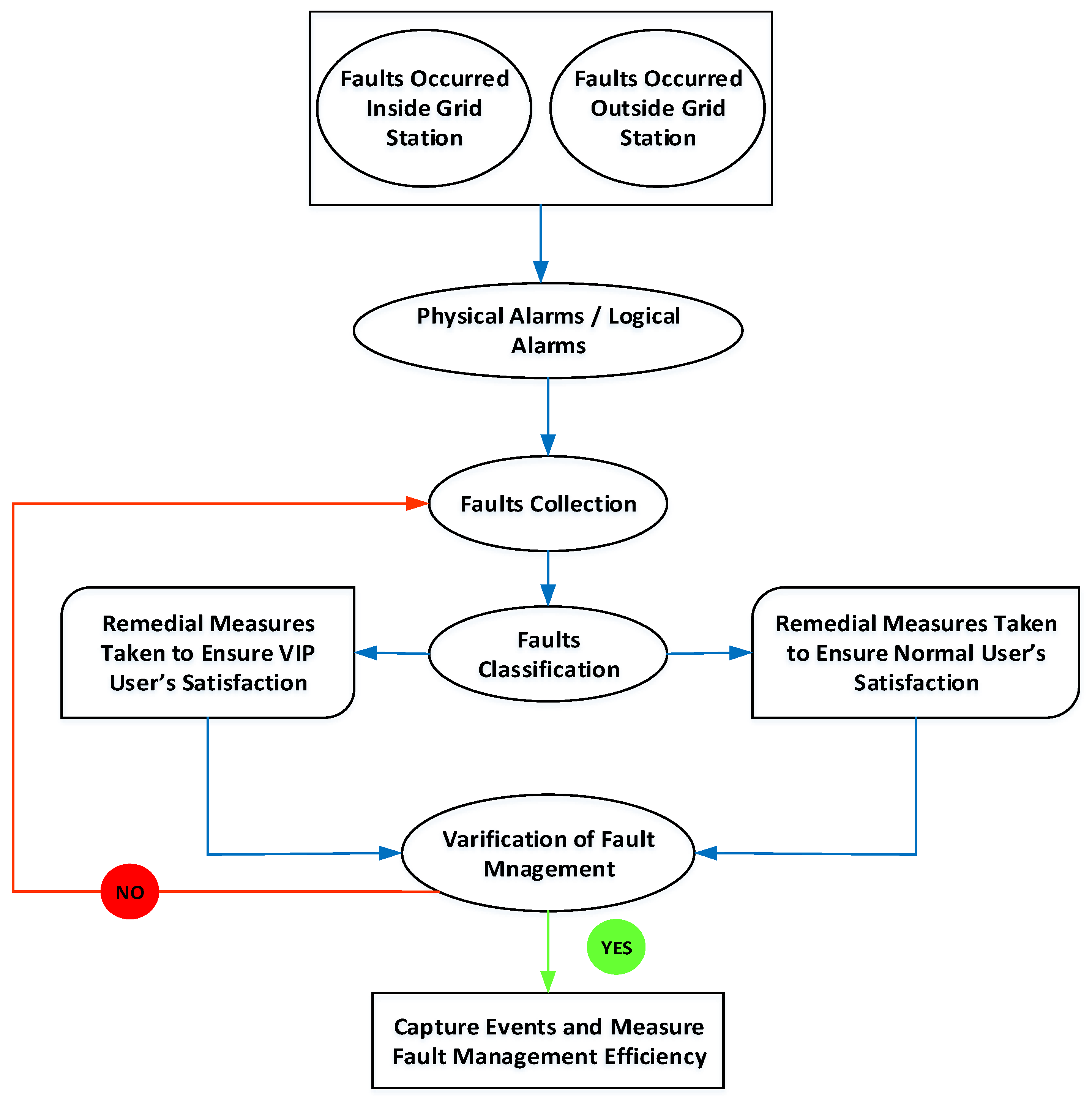
3.1. Data-Collection and Fault-Elimination Process

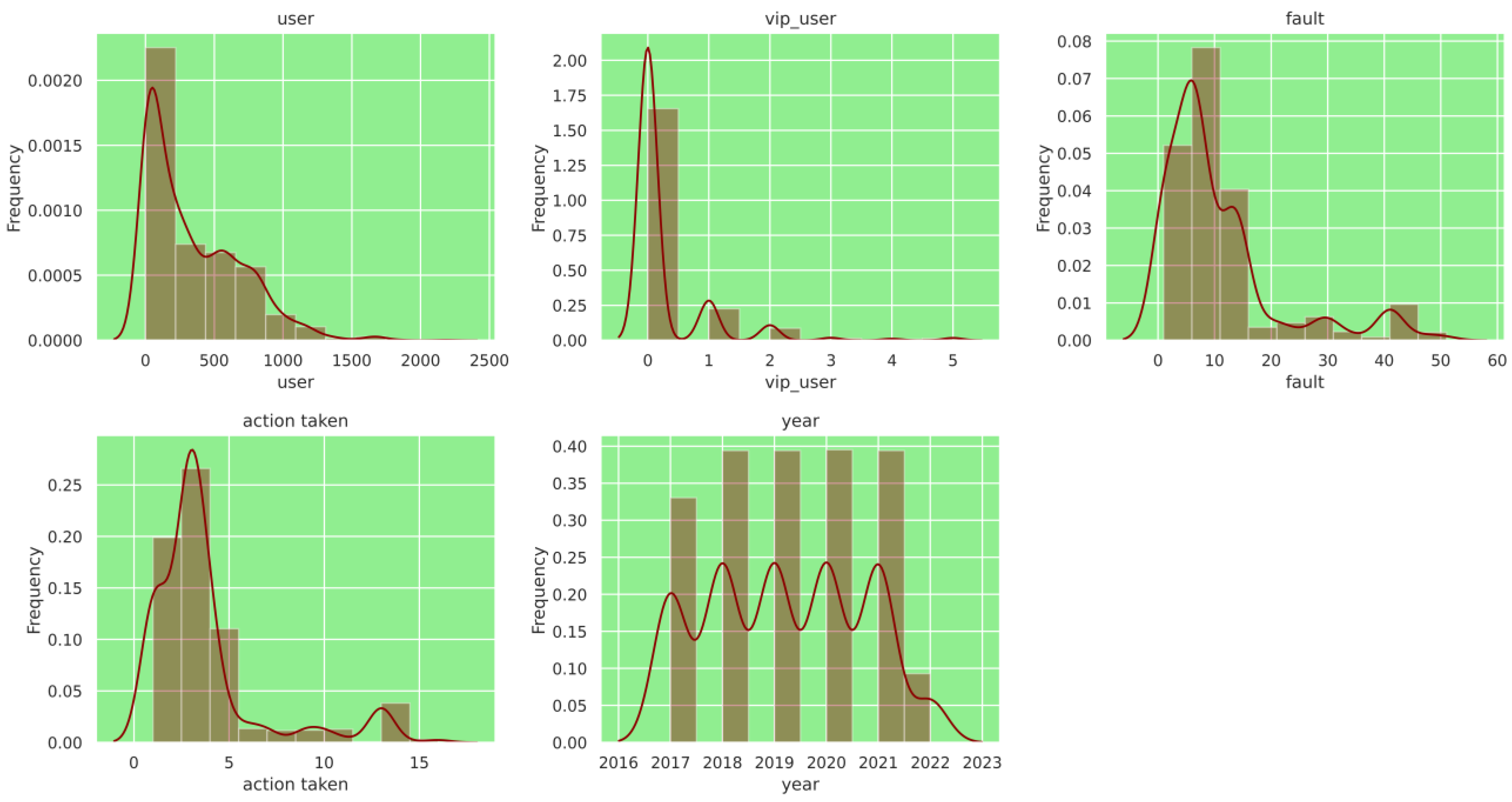
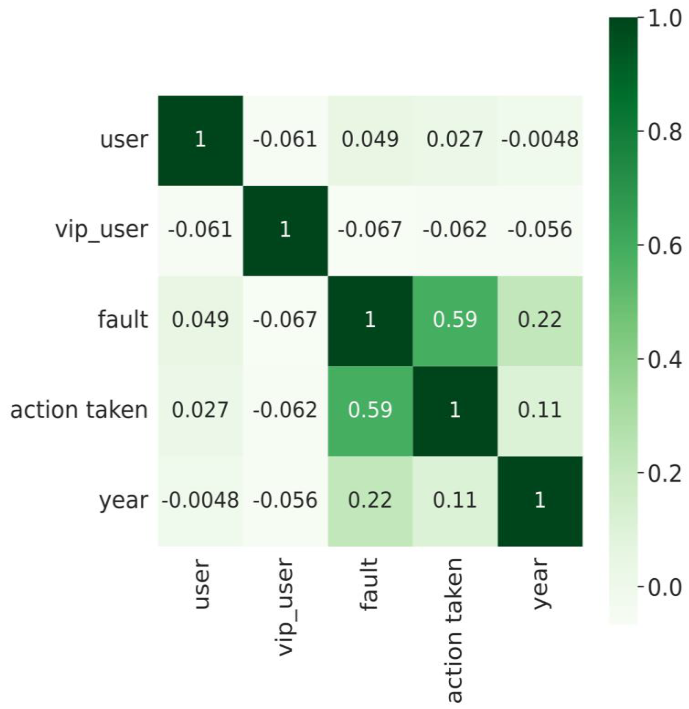
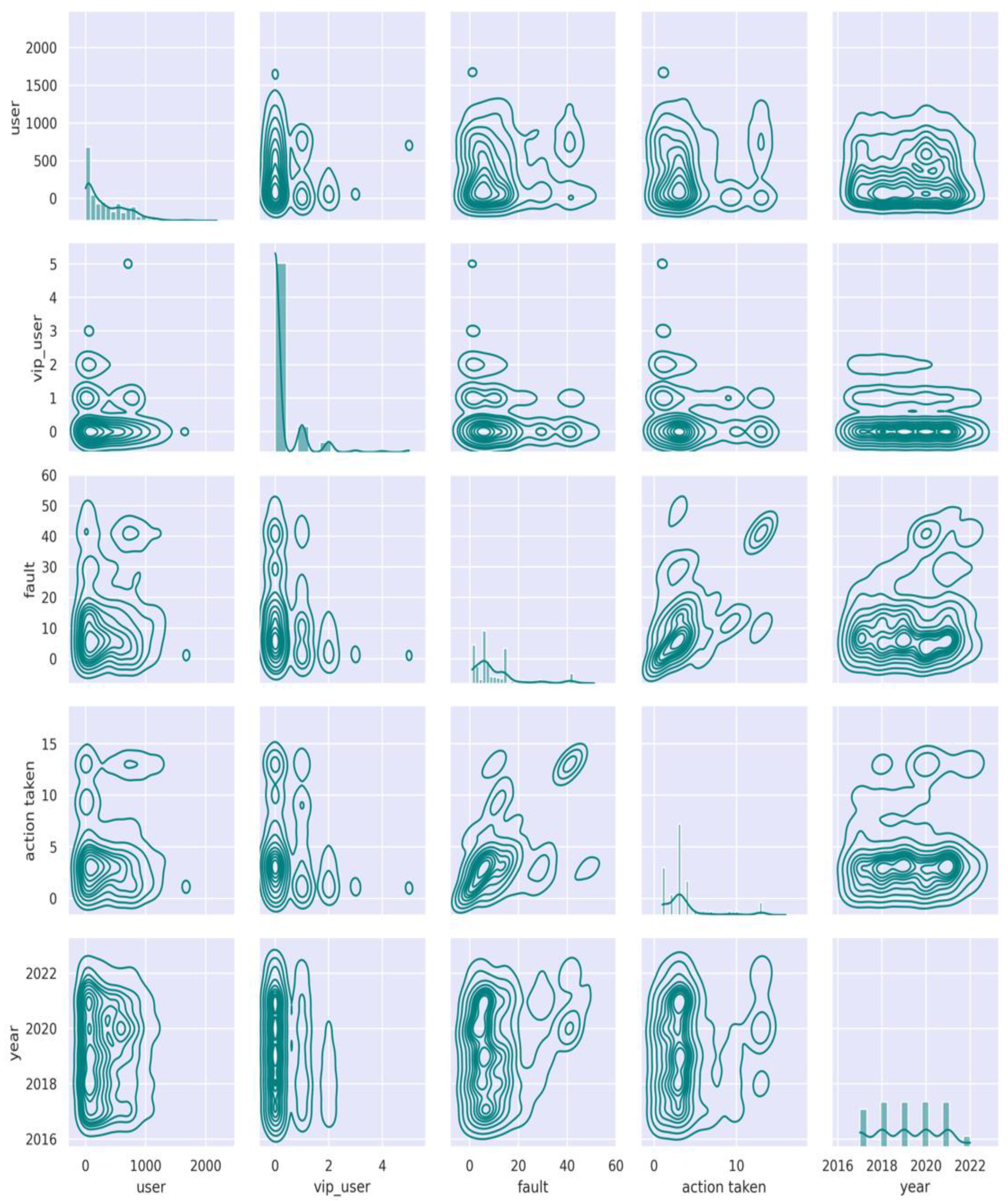
The first step to collecting data on faults outside a power grid station is determining the geographical area and type of faults to be monitored. Fault recorders, power quality monitors, visual inspections, customer reports, and system alarms are common data-collection methods. Next, the necessary equipment must be installed and configured, and parameters must be set. Data on fault events are then recorded, collected, and analyzed using software tools to identify patterns and trends. This data analysis provides insights to improve network performance by taking corrective actions or improving general infrastructure.

Similarly, to collect data on faults inside a power grid station, the first step is identifying critical equipment and systems that need monitoring. Next, monitoring equipment is installed, including sensors, meters, and other devices that record various parameters. Then, the equipment is configured, parameters are set, and data on the performance of the equipment and systems are recorded. Finally, these data are analyzed to identify patterns or trends in the occurrence of faults inside the power grid station using software tools. The insights gained from the data analysis are used to improve maintenance, reduce downtime, and identify potential problems before they become significant issues, allowing for proactive maintenance. The process of gathering information on faults and the corresponding corrective actions is illustrated in Figure 4.

3.2. Data Analysis

The histogram in Figure 5 shows the distribution of the variables in the dataset. The variable “Number of years” is continuous and ranges from 0 to 6, representing the number of years between 2017 and 2022. The variable “Number of faults occurred” ranges from 0 to 59, indicating the number of faults that occurred during this period. The histogram of this variable shows that most values fall within the range of 0 to 20, with a long tail on the right indicating some occurrences of high fault rates. The variable “Number of VIP Electricity Users” ranges from 0 to 10, indicating the number of high-priority customers. The histogram shows that the majority of values fall within the range of 0 to 2, with a few occurrences of higher values. Finally, the variable “Number of Normal Electricity Users” ranges from 0 to 2000, representing the number of regular customers. The histogram of this variable shows that most values fall within the range of 0 to 500, with a long tail on the right indicating that some customers use a siginficant amount of electricity, as shown in Figure 5.

Figure 6 presents a heat map depicting the relationships between the dataset’s variables. Normal electricity consumers have increased as the number of years since 2017 has increased, suggesting a trend towards more customers. Additionally, the number of VIP electricity consumers positively correlates with the number of regular energy users, suggesting that high-priority customers may be more likely to have more regular customers. Finally, assuming that having more high-priority clients is correlated with fewer defects, there is a modest negative association between the number of faults and the number of VIP power consumers. Overall, the heat map provides insights into the relationships between the variables in the dataset, as represented in Figure 6.

A pair plot is a graphical representation of the pairwise relationships between multiple variables. It typically shows scatter plots for each pair of variables along with their histograms on the diagonal. The purpose of the pair plot is to visualize the relationships between different variables and to identify any patterns or trends in the data, as described in Figure 7.

The scatter plots in Figure 7 illustrate the connection between each set of variables. In contrast, the histograms arranged diagonally demonstrate how each variable is distributed, and it can be seen that there is a positive connection between the number of users and the number of faults that have occurred. Additionally, there is a positive correlation between the number of VIP users and the actions that have been performed in response to the faults. It also tends to raise defects over time and show a trend of more significant action being performed against the flaws. Both of these trends are related. In general, the pair plot offers a helpful visual depiction of the interactions between the various characteristics and may be used to gain insights into the data.

All the above discussion shows that data acquired from the grid are valuable and help to proceed further. The next section, Section 4, details the results and discussion.

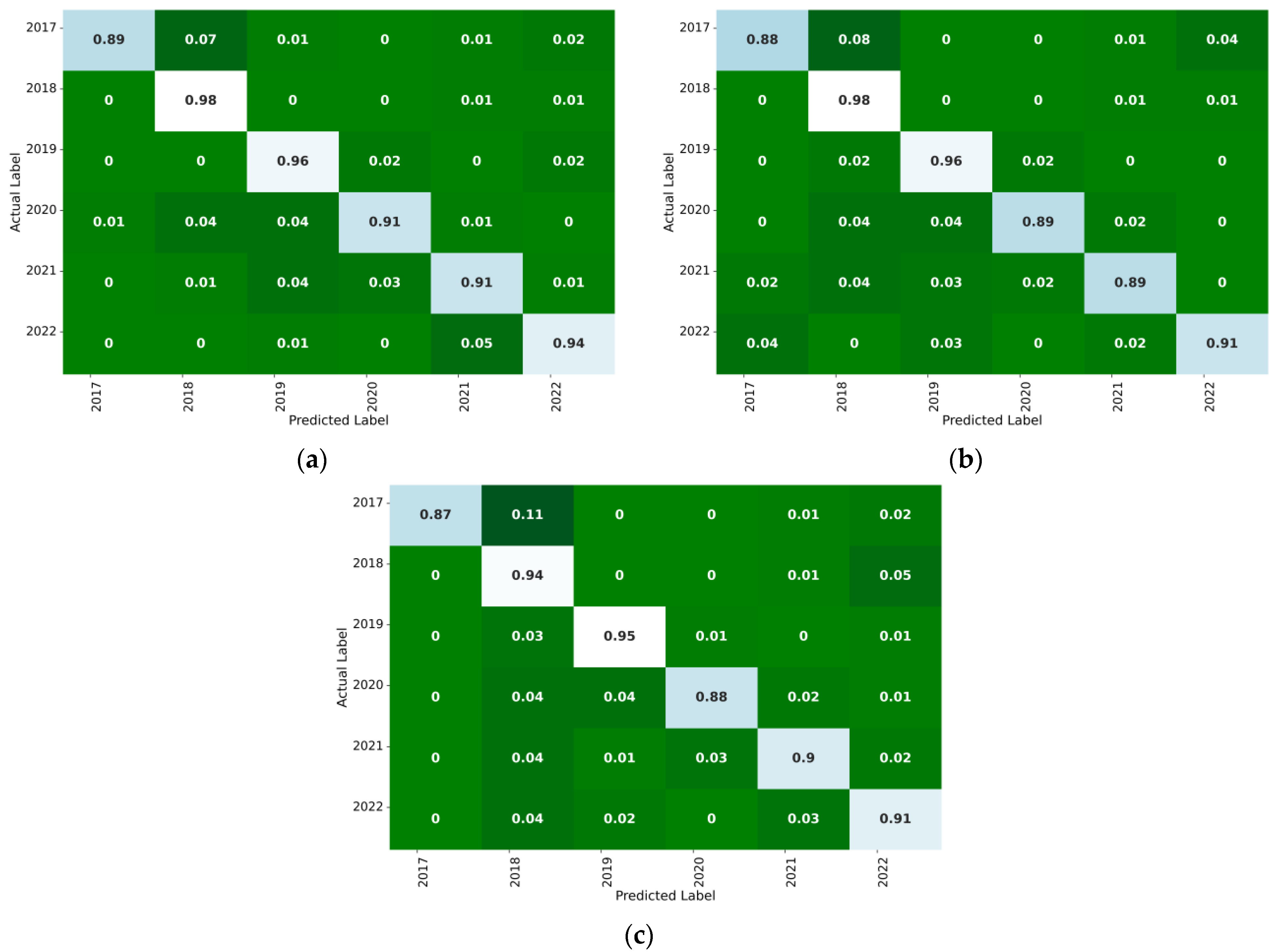
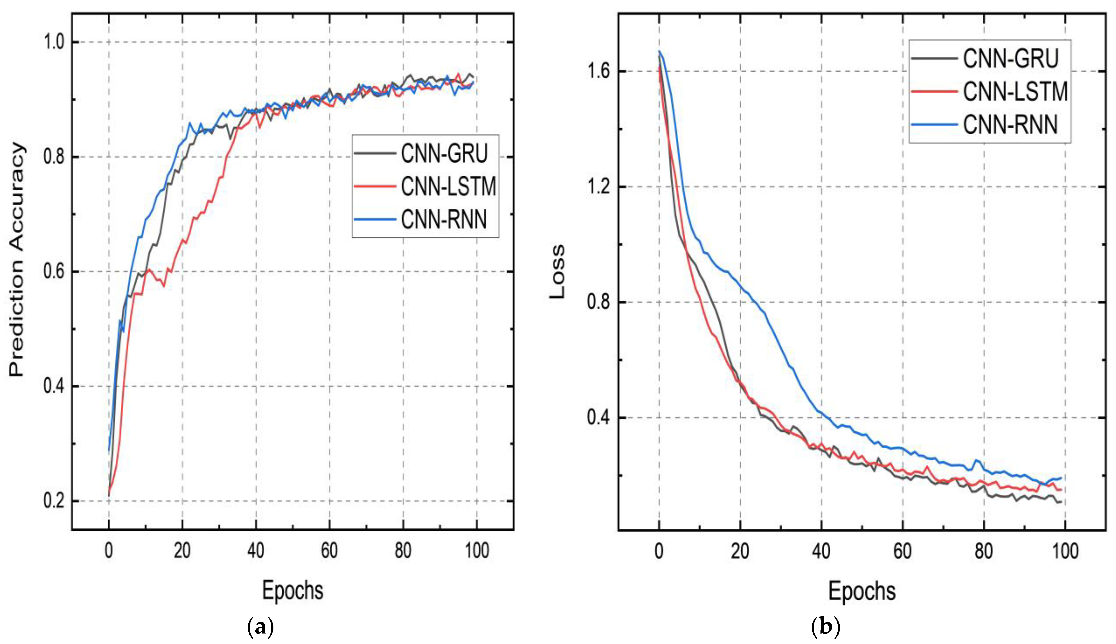
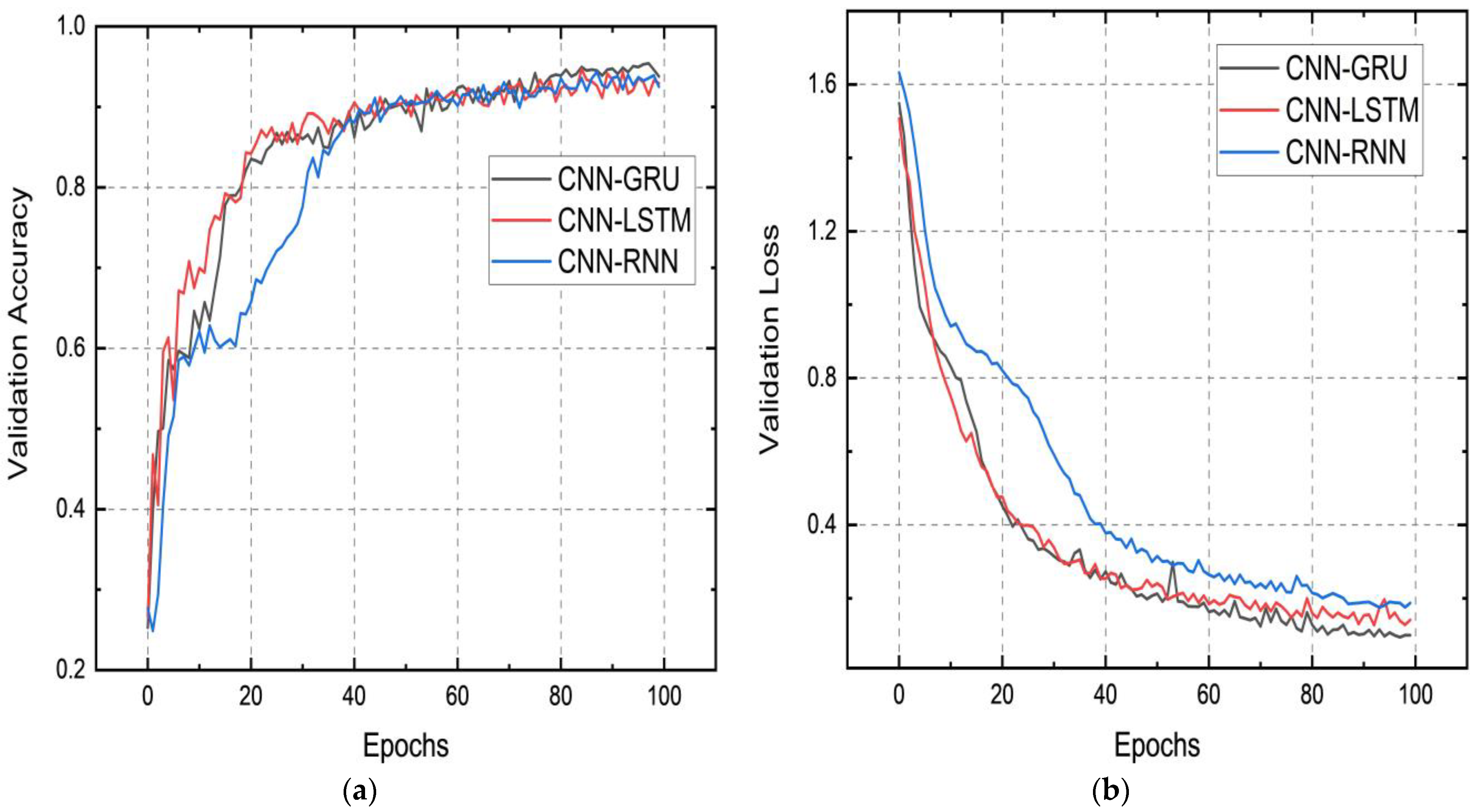
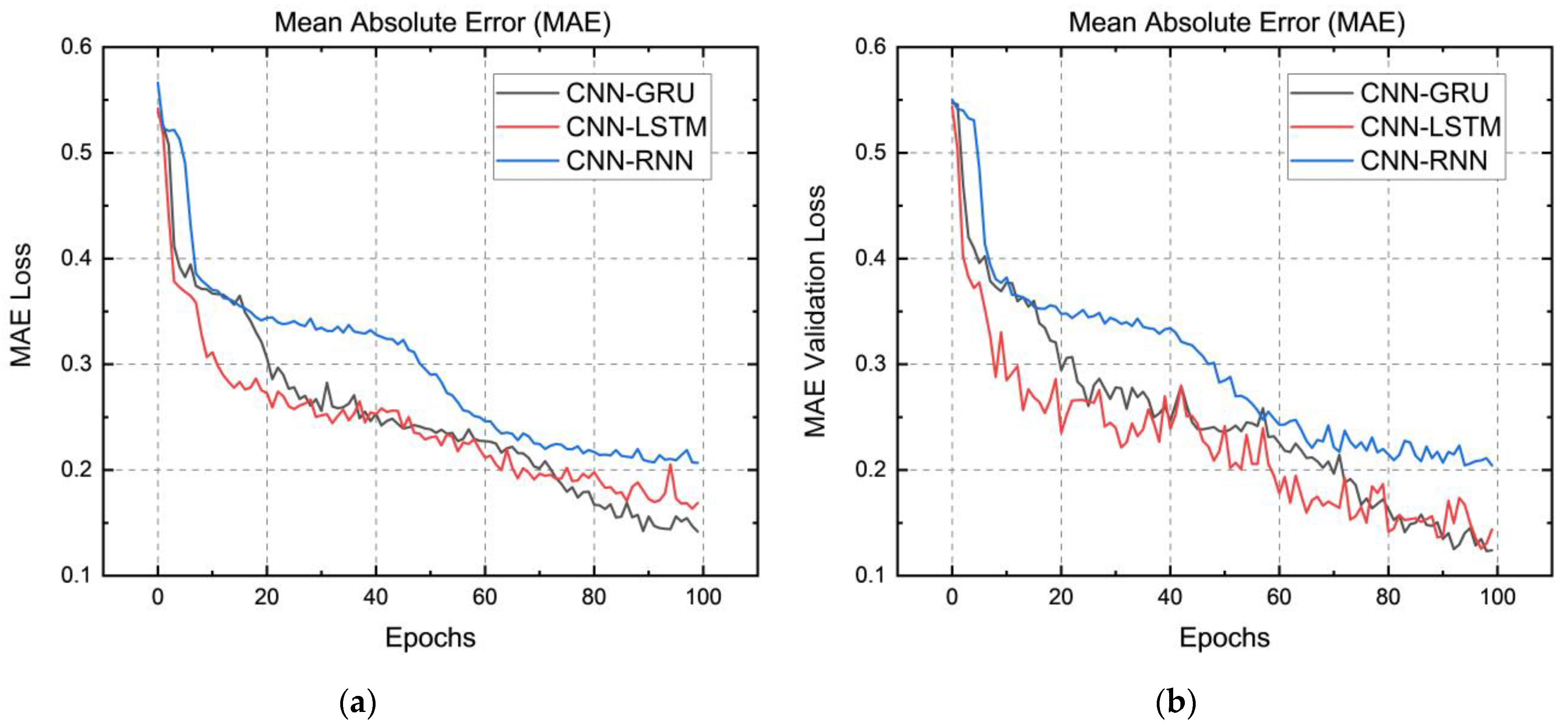
4. Results and Discussion

The confusion matrices of three different models that are utilized for fault classification prediction in real-time data are shown in Figure 8. When there is an imbalance in the number of observations that belong to each class or when there are many classes present in the dataset, a confusion matrix may be used to summarize a classification system’s efficacy. This allows us to assess the advantages and downsides of the categorization models based on the results they generated. Figure 8a depicts the confusion matrix created by comparing the actual values of the dataset to the predicted values produced by the CNN-GRU hybrid model. Compared to the other two models, the findings suggest that the model successfully predicted real positive values with the most significant percentage. This suggests that the data were categorized with fewer misleading values. The confusion matrices of the other two models, CNN-LSTM and CNN-RNN, illustrated in Figure 8b,c, respectively, exhibit the performance outcomes of these models. The CNN-GRU hybrid model outperforms the CNN-LSTM and CNN-RNN hybrid models, whereas the CNN-RNN hybrid model fares poorly.

Figure 9 shows a general flowchart representing a typical deep learning process for input data and generating output results. First, the input data go through two convolution layers before being sent to a max pooling layer. The maximum pooling layer’s output is then flattened and repeated vector-wise to prepare it for processing by the selected machine learning model. In this case, three models are selected individually after the convolution neural network (CNN) layer. To prevent overfitting, a dropout layer is applied after the selected model, and then the layer is wrapped in a bidirectional layer to allow for bidirectional processing of the input sequence. Finally, another dropout layer is applied before passing the output to two dense layers, which use a variety of activation functions to produce the final output results for comparison.

Table 1. Hybrid CNN-GRU machine learning model for fault prediction.

Model: “sequential_8”
Layer (Type)	Output Shape	Param #
conv1d_14 (Conv1D)	(None, 3, 128)	384
conv1d_15 (Conv1D)	(None, 2, 64)	16,448
max_pooling1d_7 (MaxPooling 1D)	(None, 1, 64)	0
flatten_7 (Flatten)	(None, 64)	0
repeat_vector_7 (RepeatVector)	(None, 10, 64)	0
gru_6 (GRU)	(None, 10, 200)	159,600
dropout_12 (Dropout)	(None, 10, 200)	0
bidirectional_6 (Bidirectional)	(None, 256)	253,440
dropout_13 (Dropout)	(None, 256)	0
dense_12 (Dense)	(None, 100)	25,700
dense_13 (Dense)	(None, 1)	101
Total params: 455,673
Trainable params: 455,673
Non-trainable params: 0

shows a description of a neural network model called CNN-GRU, which operates on a series of data and returns a single value. The model has a series of layers, including convolutional, max pooling, flattening, repeat vector, gated recurrent unit (GRU), dropout, bidirectional, and dense layers. The actual number of trainable parameters in the model is 455,673. The model extracts features from the input sequence using convolutional layers and processes the sequence using a GRU layer. Dropout layers are used to prevent overfitting, and a bidirectional layer processes the output of the GRU layer in both forward and backward directions. Finally, a dense layer produces the final output with a sigmoid activation function.

The CNN-LSTM sequential neural network model is shown in

Table 2. Hybrid CNN-LSTM machine learning model for fault prediction.

Model: “sequential_8”
Layer (Type)	Output Shape	Param #
conv1d_4 (Conv1D)	(None, 3, 128)	384
conv1d_5 (Conv1D)	(None, 2, 64)	16,448
max_pooling1d_2 (MaxPooling1D)	(None, 1, 64)	0
flatten_2 (Flatten)	(None, 64)	0
repeat_vector_2 (RepeatVector)	(None, 10, 64)	0
lstm_4 (LSTM)	(None, 10, 200)	212,000
dropout_4 (Dropout)	(None, 10, 200)	0
bidirectional_2 (Bidirectional)	(None, 256)	336,896
dropout_5 (Dropout)	(None, 256)	0
dense_4 (Dense)	(None, 100)	25,700
dense_5 (Dense)	(None, 1)	101
Total params: 591,529
Trainable params: 591,529
Non-trainable params: 0

. This model accepts a data sequence as its input and generates a single output. Convolutional, max pooling, flattening, repeat vector, long short-term memory (LSTM), dropout, bidirectional, and dense layers are some of the types of layers included in this model. A total of 591,529 is the maximum number of trainable parameters that may be found in the model. The model extracts features from the input sequence using convolutional layers and processes the sequence using an LSTM layer. Dropout layers prevent overfitting, and a bidirectional layer processes the output of the LSTM layer in both forward and backward directions. A dense layer produces the final output with a sigmoid activation function.

A single output is generated by the CNN-RNN sequential neural network model described in

Table 3. Hybrid CNN-RNN machine learning model for fault prediction.

Model: “sequential_8”
Layer (Type)	Output Shape	Param #
conv1d_16 (Conv1D)	(None, 3, 128)	384
conv1d_17 (Conv1D)	(None, 2, 64)	16,448
max_pooling1d_8 (MaxPooling1D)	(None, 1, 64)	0
flatten_8 (Flatten)	(None, 64)	0
repeat_vector_8 (RepeatVector)	(None, 10, 64)	0
simple_rnn (SimpleRNN)	(None, 10, 200)	53,000
dropout_14 (Dropout)	(None, 10, 200)	0
bidirectional_7 (Bidirectional)	(None, 256)	84,224
dropout_15 (Dropout)	(None, 256)	0
dense_14 (Dense)	(None, 100)	25,700
dense_15 (Dense)	(None, 1)	101
Total params: 179,857
Trainable params: 179,857
Non-trainable params: 0

. This model accepts a data sequence as its input and generates just one output. Some of the models’ components are convolutional, max pooling, flattening, repeat vector, basic recurrent neural network (RNN), dropout, bidirectional, and thick layers. The model has a total of 179,857 trainable parameters in its infrastructure. The model extracts features from the input sequence using convolutional layers and processes the sequence using a simple RNN layer. Dropout layers prevent overfitting, and a bidirectional layer processes the output of the simple RNN layer in both forward and backward directions. Finally, a dense layer produces the final output with a sigmoid activation function.

The results of this study focused on evaluating the performance of three machine-learning hybrid models, CNN-GRU, CNN-LSTM, and CNN-RNN, for fault classification and elimination in a power grid station. In Figure 10a, a graphical representation was used to visualize the prediction accuracy of these models, with the y-axis showing the prediction accuracy ranging from 0.2 to 1.0 and the x-axis indicating the number of epochs from 0 to 100. The acquired results clearly indicate that the CNN-GRU hybrid model outperformed the other two models, CNN-LSTM and CNN-RNN, in terms of prediction accuracy. This finding suggests that the CNN-GRU model can more accurately identify and eliminate faults in power grid stations. Similarly, in Figure 10b, a graphical representation is used to visualize the prediction loss of these models, with the y-axis showing the prediction loss ranging from 0 to 1.6 and the x-axis indicating the number of epochs from 0 to 100. Again, the results clearly indicate that the CNN-GRU hybrid model has the minimum loss compared to the other two models, CNN-LSTM and CNN-RNN. This finding suggests that the CNN-GRU model can effectively identify and eliminate faults in power grid stations with greater accuracy and precision, resulting in minimal prediction loss.

In Figure 11a, the proposed hybrid models are evaluated on their performance using validation accuracy as the metric. To visually represent the results, the validation accuracy is plotted against the number of epochs, ranging from 0 to 100 on the x-axis, and the validation accuracy ranges from 0.2 to 1.0 on the y-axis. The results show that all three models achieve high validation accuracy, with CNN-GRU achieving the highest accuracy, followed by CNN-RNN and CNN-LSTM. Similarly, in Figure 11b, the validation loss is plotted against the number of epochs, ranging from 0 to 100, on the x-axis. In contrast, the validation loss is displayed on the y-axis, ranging from 0 to 1.6. Again, the results demonstrate that the CNN-GRU model outperformed both the CNN-LSTM and CNN-RNN models, with the lowest validation loss observed.

In Figure 12a, a graphical representation of Mean Absolute Error (MAE) loss is depicted against the number of epochs ranging from 0 to 100. It is evident from the plot that the MAE loss exhibits a gradual decrease from 50% as the number of epochs increases. However, upon comparing the three models, the hybrid model CNN-GRU yields a minimum loss of approximately 15%, outperforming the other two models. Similarly, Figure 12b displays a graphical representation of MAE validation loss against the number of epochs ranging from 0 to 100. Again, the plot reveals a gradual decrease in MAE loss from 55% with increasing epochs. However, upon comparing the three hybrid models, it is evident that the CNN-GRU model produces the minimum validation loss for MAE, which is approximately 11%, outperforming the other two hybrid models. This is clearly visible from the graphical visualization shown in Figure 12b.

Figure 13a is a graphical representation of this evaluation, showing the relationship between MSE loss and the epoch ranges from 0 to 100. The results show that as the number of epochs increases, the MSE loss decreases gradually. The hybrid model CNN-GRU achieved the minimum MSE loss, around 5%, as shown in Figure 13a. This was significantly lower than the MSE loss achieved by the other two hybrid models evaluated in the same experiment. Similarly, in Figure 13b, the graphical representation of this evaluation shows the relationship between MSE validation loss and the number of epochs. The results show that as the number of epochs increases, the MSE validation loss decreases gradually. The hybrid model CNN-GRU achieved the minimum MSE validation loss, around 5%, as shown in Figure 13b. This was significantly lower than the MSE validation loss achieved by the other two hybrid models evaluated in the same experiment.

Earlier studies on the same dataset have been conducted to make predictions using various hybrid machine learning models. The models that were taken into consideration for this analysis were a basic Recurrent Neural Network (RNN), a Long-Short Term Memory (LSTM), and a Gated Recurrent Unit (GRU) [22]. The following metrics—Losses, Accuracy (%), MAE loss, and RMSE loss—were taken into consideration: the performance of the GRU model was superior to that of the other models, with a loss of 0.22, an accuracy of 91.69%, an MAE loss of 0.42, and the RMSE loss of 0.40. Following closely in terms of performance was the LSTM model, which had a loss of 0.21, an accuracy of 92.13%, an MAE loss of 0.37, and an RMSE loss of 0.39. The RNN model had the lowest accuracy, at 89.21%, and the most significant loss, at 0.28, with an MAE loss of 0.45 and the RMSE loss of 0.47 [22]. The GRU model demonstrated improved performance in terms of accuracy and loss, making it ideal for predicting the intended outcomes.

Table 4. Results of fault classification and fault elimination data via hybrid CNN-RNN, CNN-LSTM, and CNN-GRU models.

Hybrid Models for Prediction	Accuracy (%)	MAE Loss	Loss	RMSE Loss
CNN-RNN	92.85	0.21	0.19	0.10
CNN-LSTM	93.05	0.17	0.15	0.07
CNN-GRU	93.92	0.14	0.10	0.05
RNN [22]	89.21	0.45	0.28	0.47
LSTM [22]	91.69	0.42	0.22	0.40
GRU [22]	92.13	0.37	0.21	0.39

displays the enhanced outcomes achieved by combining RNN, LSTM, and GRU layers with Convolutional Neural Network (CNN) layers throughout this research.

The performance of each model was evaluated based on four metrics: losses, accuracy, mean absolute error (MAE) loss, and Mean Square Error (MSE) loss. The losses metric indicates the difference between the model’s predicted output and actual output. Lower losses indicate superior performance. The accuracy metric indicates the percentage of the total correct predictions. Higher accuracy indicates superior performance. Finally, the MAE and MSE loss metrics measure the absolute and squared differences between the predicted and actual output, respectively. Again, lower MAE and MSE values indicate superior performance. It can be seen that the CNN-GRU model has the best overall performance, with the lowest losses, highest accuracy, and lowest MAE and MSE values. The CNN-LSTM model also performs well, with lower losses and higher accuracy than the CNN-RNN model.

Compared to the results in [22], the models in Table 4 show significantly better performance in terms of losses, accuracy, and MAE and MSE values. Overall, the addition of CNN layers improves the models’ performance, particularly in reducing the losses and improving accuracy. In addition, the GRU and LSTM models consistently perform better than the RNN model. The results suggest that combining CNN and RNN, LSTM, or GRU layers can lead to better predictions of target variables in neural network models.

All the above findings indicate that machine learning hybrid models, particularly the CNN-GRU model, can effectively improve prediction accuracy and reduce prediction loss, enhancing the reliability and efficiency of power grid systems. Furthermore, this study suggests that the CNN-GRU hybrid model outperforms the other two hybrid models, CNN-LSTM and CNN-RNN, in terms of minimizing MSE loss. These results provide valuable insights and can guide future research in developing more accurate and efficient fault-detection and -elimination systems in power grids. However, further research is needed to validate these findings and explore the potential of other machine learning models for this application.

5. Experimental Setup Used

The experimental system that was used for this research required the usage of specific hardware and software in order to function properly. The central processor unit (CPU) that was used was an Intel(R) Core(TM) i7-10875H CPU operating at 2.30 GHz. The graphics card used was an NVIDIA GeForce RTX 2060, and it played a significant role in successfully completing the graphical activities that were necessary for the study. It was possible to save and retrieve data quickly and easily because of the system’s 16.0 GB of RAM, of which 6.0 GB was dedicated to the GPU’s memory. Our investigation was carried out using a 64-bit Windows operating system version. Python, Keras, and TensorFlow version 2.3.1 were some of the software packages that were used, and they were the ones that made it possible to carry out the necessary machine learning activities. The overall hardware and software setup provided a dependable and effective platform for carrying out the study.

6. Conclusions

The integration of renewable energy resources into smart grids is crucial for developing a more sustainable energy system and mitigating the impact of climate change. Machine learning hybrid models can play a vital role in predicting energy demand and optimizing the use of renewable energy sources. This research study emphasizes the importance of such models in improving the efficiency and reliability of power grids by detecting and eliminating faults in a timely manner, thus preventing power outages and minimizing consumer impact. The results indicate that CNN-GRU achieved the highest accuracy of 93.92% and the lowest MAE and MSE losses of 0.14 and 0.05, respectively. CNN-LSTM and CNN-RNN also performed well, with an accuracy of 93.05% and 92.85%, respectively. The research concludes that machine learning hybrid models such as CNN-RNN, CNN-LSTM, and CNN-GRU can effectively detect and eliminate faults in grid stations, facilitating the integration of renewable energy sources and improving power grid efficiency and reliability. Combining machine learning, artificial intelligence, reinforcement learning, and advanced control techniques can create strategies to forecast load, monitor and adjust output in real-time, optimize grid performance, and handle complex load variations in the future.

References

1. Fu, X.; Zhou, Y. Collaborative Optimization of PV Greenhouses and Clean Energy Systems in Rural Areas. IEEE Trans. Sustain. Energy 2022, 14, 642–656. [Google Scholar] [CrossRef]
2. Fu, X. Statistical machine learning model for capacitor planning considering uncertainties in photovoltaic power. Prot. Control Mod. Power Syst. 2022, 7, 5. [Google Scholar] [CrossRef]
3. Meng, A.; Wang, H.; Aziz, S.; Peng, J.; Jiang, H. Kalman filtering based interval state estimation for attack detection. Energy Procedia 2019, 158, 6589–6594. [Google Scholar] [CrossRef]
4. Yang, W.; Wang, M.; Aziz, S.; Kharal, A.Y. Magnitude-reshaping strategy for harmonic suppression of VSG-based inverter under weak grid. IEEE Access 2020, 8, 184399–184413. [Google Scholar] [CrossRef]
5. Ma, Z.; Guo, S.; Xu, G.; Aziz, S. Meta learning-based hybrid ensemble approach for short-term wind speed forecasting. IEEE Access 2020, 8, 172859–172868. [Google Scholar] [CrossRef]
6. Zhang, R.; Li, G.; Bu, S.; Aziz, S.; Qureshi, R. Data-driven cooperative trading framework for a risk-constrained wind integrated power system considering market uncertainties. Int. J. Electr. Power Energy Syst. 2023, 144, 108566. [Google Scholar] [CrossRef]
7. Chen, W.; Liu, B.; Nazir, M.S.; Abdalla, A.N.; Mohamed, M.A.; Ding, Z.; Bhutta, M.S.; Gul, M. An energy storage assessment: Using frequency modulation approach to capture optimal coordination. Sustainability 2022, 14, 8510. [Google Scholar] [CrossRef]
8. Eskandarpour, R.; Khodaei, A.; Arab, A. Improving Power Grid Resilience Through Predictive Outage Estimation. In Proceedings of the 2017 North American Power Symposium (NAPS), Morgantown, WV, USA, 17–19 September 2017; IEEE: Piscataway, NY, USA; pp. 1–5. [Google Scholar]
9. Jamborsalamati, P.; Hossain, M.J.; Taghizadeh, S.; Konstantinou, G.; Manbachi, M.; Dehghanian, P. Enhancing power grid resilience through an IEC61850-based ev-assisted load restoration. IEEE Trans. Ind. Inform. 2019, 16, 1799–1810. [Google Scholar] [CrossRef]
10. Barik, A.K.; Das, D.C.; Latif, A.; Hussain, S.S.; Ustun, T.S. Optimal voltage–frequency regulation in distributed sustainable energy-based hybrid microgrids with integrated resource planning. Energies 2021, 14, 2735. [Google Scholar] [CrossRef]
11. Nazir, M.S.; Abdalla, A.N.; Zhao, H.; Chu, Z.; Nazir, H.M.J.; Bhutta, M.S.; Javed, M.S.; Sanjeevikumar, P. Optimized economic operation of energy storage integration using improved gravitational search algorithm and dual stage optimization. J. Energy Storage 2022, 50, 104591. [Google Scholar] [CrossRef]
12. Bhutta, M.S.; Sarfraz, M.; Ivascu, L.; Li, H.; Rasool, G.; ul Abidin Jaffri, Z.; Farooq, U.; Ali Shaikh, J.; Nazir, M.S. Voltage Stability Index Using New Single-Port Equivalent Based on Component Peculiarity and Sensitivity Persistence. Processes 2021, 9, 1849. [Google Scholar] [CrossRef]
13. Abubakar, M.; Che, Y.; Ivascu, L.; Almasoudi, F.M.; Jamil, I. Performance Analysis of Energy Production of Large-Scale Solar Plants Based on Artificial Intelligence (Machine Learning) Technique. Processes 2022, 10, 1843. [Google Scholar] [CrossRef]
14. Sarfraz, M.; Naseem, S.; Mohsin, M.; Bhutta, M.S. Recent analytical tools to mitigate carbon-based pollution: New insights by using wavelet coherence for a sustainable environment. Environ. Res. 2022, 212, 113074. [Google Scholar] [CrossRef]
15. Zhang, X.; Chen, X.; Chen, Z. A rule-based fault detection and diagnosis method for hydropower generating units. Energies 2018, 11, 114. [Google Scholar]
16. Abbas, M.H.; Datta, R.L.; Li, S. An expert system for power transformer fault diagnosis. IEEE Trans. Power Deliv. 1999, 14, 1142–1148. [Google Scholar]
17. LeCun, Y.; Bengio, Y.; Hinton, G. Deep learning. Nature 2015, 521, 436–444. [Google Scholar] [CrossRef] [PubMed]
18. Singh, S.K.; Pardasani, K.R.; Tripathi, R.K. Review of artificial intelligence techniques for prognostics and health management of machinery systems. Mech. Syst. Signal Process. 2018, 109, 357–380. [Google Scholar]
19. Chen, N.; Shi, Y.; Zhang, C.; Chen, W. Fault detection, fault collection, and fault management using artificial intelligence and machine learning techniques: A review. IEEE Access 2019, 7, 124485–124497. [Google Scholar]
20. Hu, B.G.; Tan, G.Q.; Zhang, W.H. A review of data-driven approaches for fault detection and diagnosis in industrial processes. IEEE Trans. Ind. Inform. 2018, 14, 3204–3216. [Google Scholar]
21. Zhao, D.; Huang, Y.; Lei, Y. A survey on deep learning-based fault diagnosis of rotating machinery. IEEE Trans. Ind. Electron. 2018, 65, 4269–4281. [Google Scholar]
22. Almasoudi, F.M. Grid Distribution Fault Occurrence and Remedial Measures Prediction/Forecasting through Different Deep Learning Neural Networks by Using Real Time Data from Tabuk City Power Grid. Energies 2023, 16, 1026. [Google Scholar] [CrossRef]
23. Zhang, Y.; Zhang, L.; Jia, S. A survey of fault diagnosis methods with deep learning. J. Sens. 2019, 2019, 2936725. [Google Scholar]
24. Raza, M.F.; Iqbal, S.Z.; Iqbal, M.Z. Fault detection and diagnosis in industrial systems using machine learning techniques: A review. J. Ind. Inf. Integr. 2020, 20, 100136. [Google Scholar]
25. Zeng, D.; Song, Q.; Li, D. Machine learning and artificial intelligence for fault diagnosis and prognosis of rotating machinery: A review. Measurement 2021, 173, 108–121. [Google Scholar]
26. El-Feky, S.S.; Elsayed, S.T.; Zaher, A.H. A review of artificial intelligence applications in fault diagnosis of rotating machinery. Arch. Comput. Methods Eng. 2021, 28, 1303–1323. [Google Scholar]
27. Liu, Y.; Sun, H.; Lin, Z.; Zhang, H. Data-driven fault detection and diagnosis methods: A review. J. Process Control 2019, 73, 28–44. [Google Scholar]
28. Hohman, F.; Otterbacher, J.; Klasnja, P. Towards Interpretable Machine Learning for Healthcare: Predicting ICU Readmission Using Tree-Based Models. In Proceedings of the 2019 CHI Conference on Human Factors in Computing Systems, Glasgow, UK, 4–9 May 2019; pp. 1–12. [Google Scholar]
29. Xue, Y.; Zhang, J. Machine learning applications in power systems. IEEE Access 2018, 6, 21912–21926. [Google Scholar]
30. Bello, O.; Li, N.; Chen, W. Machine learning applications in power systems: A review. Energies 2019, 12, 1554. [Google Scholar]
31. Han, X.; Zhang, P.; Wang, H. Fault diagnosis in power systems using a hybrid convolutional and recurrent neural network model. Energies 2019, 12, 464. [Google Scholar]
32. Wang, H.; Cao, Y.; Zhou, B. Power system fault diagnosis based on convolutional neural network and gated recurrent unit. IEEE Access 2019, 7, 53627–53634. [Google Scholar]
33. Hu, Y.; Xiang, Y.; Zhang, Y. Improved fault diagnosis method for power system based on XGBoost and convolutional neural network. IET Gener. Transm. Distrib. 2019, 13, 763–770. [Google Scholar]
34. Singh, J.; Kumar, R. Hybrid support vector machine and convolutional neural network for fault detection in power transmission systems. IET Gener. Transm. Distrib. 2020, 14, 1325–1331. [Google Scholar]
35. Lu, Y.; Li, H.; Guo, Q. An improved ensemble learning model based on random forest for power system fault diagnosis. IEEE Access 2020, 8, 156478–156487. [Google Scholar]
36. Li, Y.; Xu, C. A hybrid fault diagnosis model based on PCA and SVM optimized by bat algorithm. Energies 2018, 11, 799. [Google Scholar]
37. Li, Y.; Wang, C. Fault diagnosis of power systems based on a hybrid deep belief network and self-organizing map. Energies 2020, 13, 3411. [Google Scholar]
38. Zhang, J.; Li, D.; Zhang, Y. Hybrid fault diagnosis model based on stacked denoising auto encoder and deep neural network. IEEE Access 2020, 8, 114114–114122. [Google Scholar]
39. Sun, L.; Cai, X. A hybrid power transformer fault diagnosis model based on wavelet transform, PCA, and BP neural network. Energies 2021, 14, 306. [Google Scholar]
40. Lv, T.; Wang, X.; Li, Y. A hybrid model for short-term load forecasting based on deep learning and ARIMA. Appl. Sci. 2020, 10, 1284. [Google Scholar]
Figure 1. Proposed strategy to find efficient hybrid model for fault prediction and fault elimination at power grid station.
Sustainability 15 08348 g001
Figure 2. The structure of a convolutional neural network.
Sustainability 15 08348 g002
Figure 4. Data-collection process and remedial action taken against faults.
Sustainability 15 08348 g004
Figure 5. Histogram as per collected data from grid station.
Sustainability 15 08348 g005
Figure 6. Heat map as per collected data from grid station.
Sustainability 15 08348 g006
Figure 7. Heat map as per collected data from the grid station.
Sustainability 15 08348 g007
Figure 8. Confusion matrix results of (a) CNN-GRU hybrid model; (b) CNN-LSTM hybrid model; (c) CNN-RNN hybrid model.
Sustainability 15 08348 g008
Figure 9. Proposed general framework for hybrid models.
Sustainability 15 08348 g009
Figure 10. Graphical visualization of (a) Prediction accuracy of proposed hybrid models; (b) Prediction loss of proposed hybrid models.
Sustainability 15 08348 g010
Figure 11. Graphical visualization of (a) Validation accuracy of proposed hybrid models; (b) Validation loss of proposed hybrid models.
Sustainability 15 08348 g011
Figure 12. Graphical visualization of (a) Mean Absolute Error loss of proposed hybrid models; (b) Mean Absolute Error validation loss of proposed hybrid models.
Sustainability 15 08348 g012
Figure 13. Graphical visualization of (a) Mean Square Error loss of proposed hybrid models; (b) Mean Square Error validation loss of proposed hybrid Models.
Sustainability 15 08348 g013