A Hybrid Brain Storm Optimization Algorithm to Solve the Emergency Relief Routing Model

Abstract

Due to the inappropriate or untimely distribution of post-disaster goods, many regions did not receive timely and efficient relief for infected people in the coronavirus disease outbreak that began in 2019. This study develops a model for the emergency relief routing problem (ERRP) to distribute post-disaster relief more reasonably. Unlike general route optimizations, patients’ suffering is taken into account in the model, allowing patients in more urgent situations to receive relief operations first. A new metaheuristic algorithm, the hybrid brain storm optimization (HBSO) algorithm, is proposed to deal with the model. The hybrid algorithm adds the ideas of the simulated annealing (SA) algorithm and large neighborhood search (LNS) algorithm into the BSO algorithm, improving its ability to escape from the local optimum trap and speeding up the convergence. In simulation experiments, the BSO algorithm, BSO+LNS algorithm (combining the BSO with the LNS), and HBSO algorithm (combining the BSO with the LNS and SA) are compared. The results of simulation experiments show the following: (1) The HBSO algorithm outperforms its rivals, obtaining a smaller total cost and providing a more stable ability to discover the best solution for the ERRP; (2) the ERRP model can greatly reduce the level of patient suffering and can prioritize patients in more urgent situations.

1. Introduction

This study was partly motivated by the emergency relief problem caused by the coronavirus disease 2019 (COVID-19). At the end of 2019, pneumonia of an unknown origin was detected and was contagious. Afterward, it showed an outbreak situation and rapidly expanded its contagious range, and a global epidemic occurred. Various countries have been trying to end the outbreak for over two years, but with little success. As of September 2022, more than 6 million people worldwide have died from COVID-19, and more than 600 million people have been diagnosed with the coronavirus. Most regions exhibited varying degrees of inadequate emergency medical services. To prevent the further spread of the outbreak, traffic control was implemented in many of the heavily infected areas. The lack of medical services in these areas is further exacerbated by the severe decline in the efficiency of the logistics centers. Due to this, ERRP is receiving more and more attention.

The emergency relief problem has been thoroughly studied by many academics, extending to the construction of relief models and relief route selections. To ensure the effectiveness of relief operations, indicators, such as equity, efficiency, and efficacy, need to be factored into emergency relief models [1]. Taking into account dual-target, multi-modal, and multi-commodity situations and road reliability in times of reduced capacity can help improve the efficiency of casualty transport in disaster areas [2]. At the same time, the location of the warehouse has some influence on vehicle routes. A suitable warehouse location can speed up the efficiency of rescue vehicles to a certain extent [3]. In the specific context of emergencies, the time sensitivity of the post-disaster routing problem can be high [4]. By dispatching assessment vehicles, establishing an assessment and response system [5], and validating the needs identified by social media [6], rescue needs can be predicted more accurately. The emergency repair of the damaged road network after a disaster [7] is highly important in the implementation of relief operations. Mobile Internet networks can be applied to disaster relief scenarios to ensure communication between rescuers and casualties, and to achieve improved connectivity in small-scale disaster areas [8]. The emergency relief problem has been examined from many perspectives by the academics described above, and several feasible optimization strategies for emergency relief have been proposed. There are only some optimizations that have been made to models, which have not made the solutions for the ERRP faster or more accurate. Furthermore, the relief distribution problem in emergencies has received little attention.

ERRP is a complex optimization problem that arises in emergency management scenarios, such as natural disasters or humanitarian crises. The objective of ERRP is to minimize rescue time, maximize the number of people whose probability of survival exceeds a marginal level, or minimize loss of life and human suffering under various constraints, such as capacity constraints and time windows [9,10,11]. Post-disaster emergency relief and material distribution can be viewed as a specific type of vehicle routing problem (VRP) with time windows, which has garnered considerable attention in the field of path selection. VRP with time windows plays a crucial role in various aspects of our daily lives, ranging from small delivery arrangements for take-away and express delivery to large-scale deployment of materials across different regions.

While traditional VRP models can be adapted for scheduling emergency supplies, such models have significant limitations when it comes to emergency relief and material distribution. In contrast to solving VRPs, where minimizing total cost and time is typically the main objective, solving the ERRP requires more consideration of the degree of suffering of the patients or casualties. Priority must be given to patients in more critical conditions. Consequently, a realistic gap exists between traditional VRP models and ERRP models. To address this issue, we have proposed a model that incorporates the concept of deprivation cost to prioritize support for patients in urgent situations [12]. The proposed ERRP model considers time windows, vehicle load capacity, and deprivation cost. By using this model, we can more accurately simulate the actual post-disaster material distribution scenario and obtain a more realistic solution that meets the needs of emergency relief operations.

The BSO algorithm, a novel intelligent optimization computing technique, has demonstrated its benefits in handling large-scale, high-dimensional, multi-peak function issues that are challenging for traditional optimization methods to address [13]. In the fight against COVID-2019, the BSO can be used to analyze the severity of COVID-19 in terms of the coagulation index [14] or to perform feature selection for COVID-19 classification [15]. In predictive computing, the BSO algorithm has advantages in terms of fast velocity, accuracy, and reliability in predicting protein structures [16] and also demonstrates the effectiveness in the fast prediction of fixations [17]. In the VRP, the BSO algorithm shows a strong ability to explore space [18]. In addition, the application of the BSO algorithm can be extended to image classification [19] and electromagnetic classification [20]. Since BSO demonstrates powerful performance, in this study, we use the BSO algorithm to solve the model. However, since the original BSO algorithm generates new solutions randomly with fixed probability, searching for the solution space is slow and unstable. For this reason, many scholars have made improvements to the BSO algorithm. The performance of the BSO algorithm can be improved on different autonomous system (AS) ontology alignment tasks using the idea of the compact co-evolutionary [21]. To reduce the limitation of the algorithm’s exploration capability by generating new individuals, the alternative search pattern strategy can be used to control the transition between grid-based search operators and the BSO. In this way, the BSO’s effectiveness in terms of solution quality and population diversity will significantly improve [22]. Adding a reinforcement learning mechanism to the BSO algorithm can improve the comprehensive performance [23]. The BSO algorithm can also be enhanced to find better or explore viable evolutionary routes and speed up the convergence by using the improved Nelder–Mead and elite learning mechanism [24]. Moreover, combining the BSO algorithm with the orthogonal learning design [25] or the SA algorithm [26] can enhance the algorithm’s performance as well. The BSO algorithm, as an emerging metaheuristic algorithm, has attracted significant attention from scholars, who have studied and improved it to promote its application and development in various fields. However, despite these efforts, there are still certain shortcomings that need to be addressed. For example, while the improved BSO algorithms have shown some improvements in convergence speed, they still tend to converge relatively slowly. Additionally, it remains challenging to escape from local optima when using these algorithms.

LNS, initially proposed by Shaw [27], is a metaheuristic approach that gradually improves an initial solution by iteratively destroying and repairing the solution. The destroy method removes a portion of the current solution, and the repair method rebuilds the destroyed portion. The destroy method often includes stochastic elements to ensure that different portions of the solution are removed each time it is applied. One popular approach is to scan all free customers and insert the one with the lowest insertion cost, repeating until all customers are served [28]. LNS is widely used in solving various types of VRP problems due to its powerful local search capability. Goeke et al. [29] improved the consistency of solution arrival time by incorporating LNS into solving the consistent vehicle routing problem (ConVRP). The inclusion of LNS in the model can also improve the heterogeneous fleet VRP with draft limits, which contains a large number of objectives and has high robustness [30]. The LNS framework is used to search for efficient solutions that effectively find high-quality non-dominated solutions [31]. In general, LNS has a powerful local search capability to find the optimal solution within a certain range. It is also because of this that the LNS algorithm is prone to fall into local optimality.

SA was first introduced by N. Metropolis et al. [32]. The SA method is based on the analogy of cooling liquid metals to form crystals, called annealing. At high temperatures, liquid molecules have higher energy levels, making it easier for them to move towards other molecules. When the temperature is lowered, the molecules arrange themselves to find configurations with lower energy levels. By slowly reducing the temperature, the molecules can self-regulate and reach a stationary or stable state with the lowest energy level. SA is widely used in solving VRP problems. An improved SA algorithm with a crossover operator, called ISA-CO, is proposed to solve the capacitated vehicle routing problem (CVRP) [33]. Incorporating SA in the search process yields better initial solutions. To account for multiple cross-docks and heterogeneous fleets in distribution systems, an adaptive neighborhood simulated annealing algorithm is proposed, which implements an adaptive mechanism to select neighborhood moves to improve the solution [34]. The SA algorithm has a global exploration ability that can compensate for the local optimality issue in LNS.

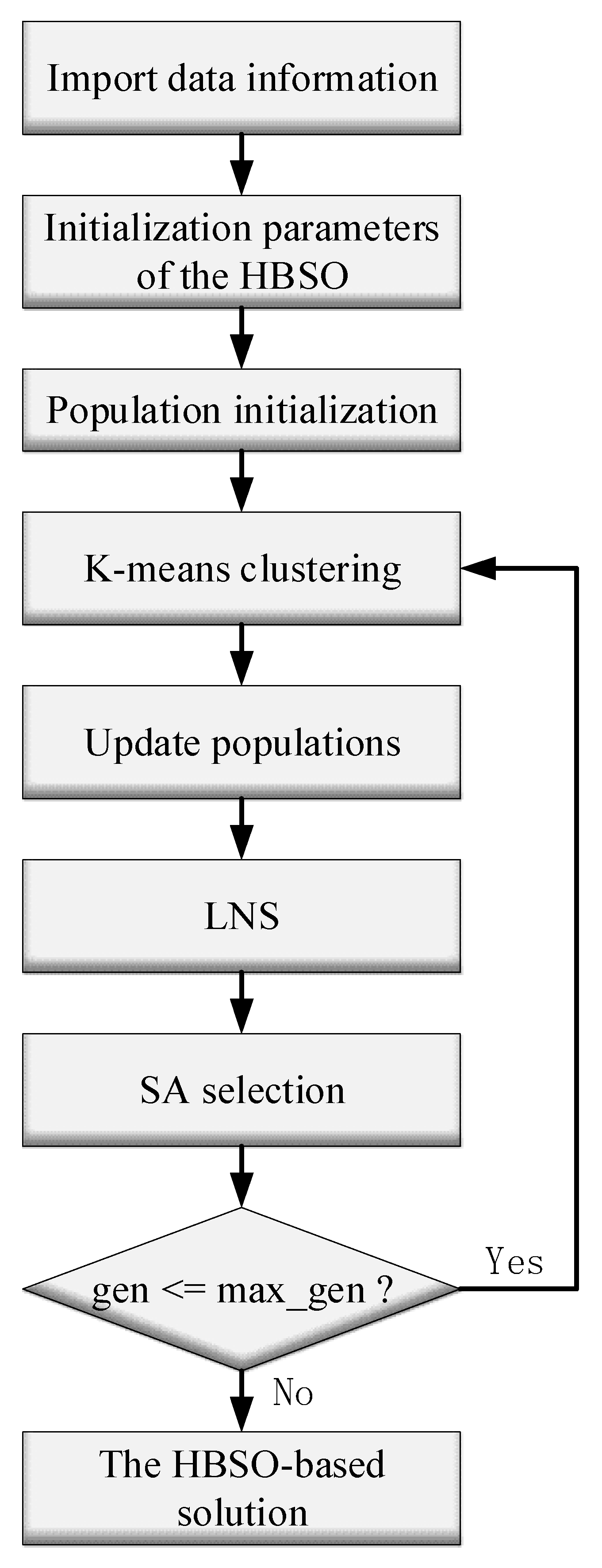
Considering the powerful search capability of LNS, it can solve the shortcoming of the BSO algorithm in finding new solutions with random values and speed up the convergence speed. SA, on the other hand, can guarantee the global exploration and avoid falling into local optimum. We establish a hybrid BSO algorithm based on the LNS and SA, and the ERRP solution model is then solved using the HBSO algorithm. All abbreviations in this article are shown in Abbreviations Part.

The main innovations of this study are as follows:

(1)

An emergency relief routing model is established, in which the dynamic distress of patients (the deprivation cost) is introduced. Patients in critical conditions can now obtain priority assistance.

(2)

The LNS and SA algorithms’ concepts are included in the BSO algorithm, accelerating the convergence and enhancing the algorithm’s ability to avoid falling into the local optimum trap.

(3)

The process of using random steps to find new solutions is changed to enhance the search capability in the BSO algorithm.

This paper is organized as follows. Section 2 describes the related work of ERRP. Section 3 introduces the description and model for the ERRP. Section 4 presents the main elements of the HBSO algorithm. Section 5 briefly describes the solution strategy of the HBSO algorithm to the ERRP. Section 6 contains the experiments, corresponding results, and analysis. Section 7 concludes the paper.

2. Related Work

2.1. The Emergency Relief Problem

There are various performance metrics defined for the distribution of relief goods. Efficiency measures the extent to which the objective of rapid and adequate distribution is achieved, while equity measures the degree to which all recipients are served in a comparable manner. Examining how efficiency, efficacy, and equity influence the structure of vehicle routes and resource allocation is an important question [1]. After a disaster, some routes may become partially or entirely inaccessible, leading to a need for a new bi-objective, multi-modal, and multi-commodity model. This model considers reliability as one of its parameters to aid managers in making more informed decisions [2]. In emergency logistics, quick and well-informed decisions regarding warehouse locations and vehicle routes are essential for post-disaster relief efforts. Xiaowen Wei et al. designed a distribution system for a homogeneous fleet of rescue vehicles that considered a set of candidate warehouse locations to deliver relief supplies to disaster areas after an incident [3]. The assessment routing problem involves sending teams to different communities to assess damage and relief needs after a disaster. To address time sensitivity, a continuous approximation method is proposed [4]. As part of the response operation, post-disaster assessments are critical. Selecting roadway segments and population points for assessment activities should be based on their value to the continuous response operations [35]. Forecasting methods for estimating rescue needs are currently inadequate. This issue can be addressed by dispatching assessment vehicles to the affected region during a disaster. A Markov decision process is proposed as a multi-intelligence assessment and response system to enhance emergency response operations and reduce fatalities [5]. Social media can improve situational awareness during disaster relief by quickly identifying needs. However, needs identified through social media must be validated initially, as some may be inaccurate. This validation challenge can hinder their use during disaster response decisions [6]. In the aftermath of a disaster, the lack of basic necessities, such as clean water, food, shelter, and medical care, often leads to an increase in the number of casualties. A critical issue that affects the distribution of relief supplies is the condition of the road network following the disaster. The dispatch and routing of repairers to optimize accessibility to towns and villages in need of humanitarian relief is a critical problem, commonly referred to as the network repairer dispatch and routing problem [7]. To reduce the negative effects of disasters on human health, it is essential to prioritize which roads to clean to transport relief items. Debris removal has been studied mostly during the recovery or reconstruction phase of a disaster, but Nihal Berktaş et al. aimed to provide a solution to the debris removal problem during the response phase [36]. Mobile ad-hoc networks (MANETs) are well-suited for disaster relief scenarios that often lack network infrastructure, and a proactive routing protocol called MQ-Routing has been proposed to maximize the minimum node lifetime and quickly adapt to network topology changes [8]. Effective communication between local authorities, first responders, and the population in disaster-affected areas is critical to the success of relief operations. However, the typical telecommunication network infrastructure may be damaged or not working properly, resulting in a lack of communication. To address this issue, a device-to-device based framework is proposed to organize users in the disaster area into user clusters and select a gateway for each cluster to maximize energy efficiency [37]. The intelligent collaborative evolution customized industrial Internet of Things (IoT) has also demonstrated superiority and stability in this regard [38]. Finally, to protect against various attacks that may occur in distributed and resource-limited networks, a resilient and secure device-to-device communication framework for emergencies called RESCUE has been proposed, which provides comprehensive protection against common attacks [39].

Several perspectives have been explored in the study of emergency relief, resulting in the proposal of various feasible optimization strategies. However, existing research mainly focuses on the enhancement of relief models and the development of relief systems, with little emphasis on expediting and improving the accuracy of emergency relief solutions. Moreover, the issue of relief distribution during emergency situations has received limited attention.

2.2. Route Optimization for Emergency Relief

Academics have studied current emergency relief routing issues to identify precise solutions. In the context of the traveling salesman problem (TSP) and vehicle routing problem (VRP), two alternative objective functions are available: one for minimizing the maximum arrival time (minmax) and one for minimizing the average arrival time (minavg). Campbell et al. investigated the impact of using these alternative objectives and found that routing costs could increase [40]. Computational experiments were conducted to identify instances where TSP and VRP solutions significantly differed from optimal minmax and minavg solutions. Coordinating vehicle routes in post-disaster mass distribution and evacuation activities can increase the effectiveness of material relief. This can be accomplished by taking into account the three objective functions in the model: maximizing the total agency utility, maximizing the worst agency utility, and minimizing the deviation between the best and worst utility [41], or by establishing hierarchical clustering and routing procedures [42]. Setting up a supply system of intermediate warehouses [43] and setting demand parameters as fuzzy variables [44] can improve fault tolerance when providing relief operations. While focusing on rescue efficiency, it should also reduce additional traffic congestion [45]. When assigning relief operations, relief vehicles with different functions should be coordinated reasonably [46]. In computing relief routes, greedy heuristics [47], extended insertion algorithms, and the tabu search [48] are often used for large-scale emergency relief problems. For relief distribution problems that consider travel time, total cost, and the reliability of bulk delivery [49], genetic and differential evolutionary algorithms can be used to solve them. Scatter search and variable neighborhood search could be used to speed up the solving process [50]. Finally, the fast and fair distribution of supplies is the key to successful relief operations [51]. Multi-attribute decision-making techniques [52] and rolling optimization techniques [53] can help improve the reliability of the selected routes.

The aforementioned studies have made significant contributions to path selection. However, in the context of ERRP, factors beyond minimizing cost and time must be considered. Prioritizing patients in critical conditions is crucial during ERRP operations. Therefore, we propose a model that incorporates deprivation cost to simulate relief needs more accurately. The proposed ERRP model considers time windows, vehicle load capacity, and deprivation cost to create a more precise simulation of the actual post-disaster material distribution scenario.

3. The Emergency Relief Routing Problem

3.1. Problem Description

Taking the 2019 epidemic as the background, we consider the following emergency relief process: a relief vehicle k departs from the emergency logistics center ($O$), delivers and collects a certain number of supplies for the infected (hereafter refers as patients), and finally returns to the emergency logistics center. When providing and collecting supplies, it is necessary to reach the patient’s location within the time window of the patient $i$. The patient’s deprivation cost is ${DC}_i$, the number of supplies that need to be provided is $d_i$, to be collected is $P_i$, and the time spent on the relief operation is $s_i$. The patient can be reached before the left time window ($a_i$), but the relief operation cannot be performed until his left time window. It is not allowed to arrive at the patient after the right time window ($b_i$). When considering the relief routes, the shortest total travel distance is calculated, and the patient’s deprivation cost is considered. The deprivation cost increases as the patient’s waiting time increases, starting from his left time window. It is also necessary to calculate the default cost of the vehicle violating the patient’s time window ($q$) and the default cost of breaking the load capacity ($w$, the maximum loading of the vehicle is $C$). Thus, the objective function consists of the total travel distance, the deprivation costs, and the default costs multiplied by their respective coefficients. The relief vehicle needs to depart and return within the time window of the emergency logistics center (the left time window is $E$, the right time window is $L$), the time of departure is $w_k$, and the loading at this time is denoted as $L_{ok}$. The vehicle travels at a constant speed $v$.

Table 1. The parameters in the model for the ERRP.

Parameter Symbols	Parameter Meaning
$c_{ij}$	The distance between patient $i$ and patient $j$
$v$	Travel speed of the relief vehicle
$s_i$	Operation time for patient $i$
$t_{ij}$	Travel time from patient $i$ to patient $j$
$a_i$	The left time window for patient $i$
$b_i$	The right time window for patient $i$
$E$	The left time window for the emergency logistics center
$L$	The right time window for the emergency logistics center
$d_i$	Distribution demand of patient $i$
$P_i$	Recovery demand of patient $i$
$C$	The maximum loading of the relief vehicle
$M$	A large enough positive number
$\alpha$	Coefficient of the penalty function for exceeding the capacity restriction
$\beta$	Coefficient of the penalty function for exceeding the time window restriction

displays the model’s input parameters, and

Table 2. The variables in the model for the ERRP.

Variable Symbols	Variable Meaning
$w_{ik}$	Start time of the operation to patient $i$ for vehicle $k$
$L_{ok}$	Current loading of the vehicle $k$ when leaving the emergency logistics center
$L_i$	Current loading of the vehicle after operating on patient $i$
$x_{ijk}$	Whether vehicle $k$ departs from patient $i$ to patient $j$ (yes, $x_{ijk}=1$; no, $x_{ijk}=0$)
${DC}_i$	Deprivation cost of patient $i$ when the vehicle arriving
$q$	The sum of the default costs associated with exceeding the vehicle capacity constraint for each relief route
$w$	The sum of the default costs associated with each relief route exceeding the time window restriction

shows the model’s variables.

3.2. Deprivation Cost

This paper is based on the premise that commercial and humanitarian logistics have a fundamental difference. Commercial logistics prioritize delivery strategies based on efficiency and customer satisfaction in a supply–demand balanced or surplus environment. Conversely, humanitarian logistics operations aim to minimize the social cost of disasters in situations of severe shortage. This necessitates prioritizing assistance to those who need it the most within a given timeframe.

When conducting emergency relief, speed and efficiency are considered as the priority. In previous studies, scholars mostly used the objective function values of total time and total travel distance. They used the total time to gauge the efficiency of relief operations and the total travel distance to gauge whether relief routes were cost-saving. Few scholars have considered the degree of patients’ suffering. In emergency relief operations, the longer the waiting time, the higher the degree of patients’ suffering, and the less likely they are to be successfully rescued. To ensure patients’ safety, the patient should be reached before the degree of suffering reaches a dangerous level. From this perspective, the suffering of patients at the time of receiving rescue operations can also measure the effectiveness of relief operations.

José Holguín Veras et al. defined the deprivation cost as an economic assessment of human suffering [12]. While logistics costs can be estimated using standard cost estimation techniques, the most appropriate approach to reflect the impact of a delivery strategy on a population is by formally estimating a deprivation cost function. This function represents the economic cost of human suffering as a function of the amount of time a person is without a particular good or service. Although this estimate is based on economic evaluation techniques, the authors suggest that it is superior and preferable to the use of the alternative measures suggested in the literature. Then, they determined the appropriate basis for deprivation cost estimation. The objective functions they used are as follows:

$${\Psi }_T^{CP}\left(X,T\right)={\Omega }_T\left(X,T\right)+\sum _{i=1}^N\sum _{j=1}^J\rho y_{i{t}_j}$$

(1)

$${\Psi }_T^{CP}\left(X,T\right)={\Omega }_T\left(X,T\right)+P_T(X,T)$$

(2)

where $X$ is a solution to the problem, $T$ is the time frame for completing all activities, $N$ is the set of all nodes, $J=\left|X\right|$, $\rho$ represents the penalty imposed each time that the specified service level is not met, ${\Omega }_T\left(X,T\right)$ computes the total logistic cost, if the specified service level is not met, the binary variable $y_{i{t}_j}$ has a value of 1 and a value of 0 otherwise, $P_T(X,T)$ is the total penalty imposed by implementing $X$ within the planning horizon $T$, and ${\Psi }_T^{CP}\left(X,T\right)$ is the deprivation cost under a constant penalty model. Among them, they use the following deprivation cost curve, as shown in Figure 1.

3.3. Building the Model

When constructing the ERRP model, the relief vehicle can arrive at the patient before the left time window, but it must wait until the left time window to operate for the patient. The relief vehicle is not permitted to reach the patient after the right time window.

Therefore, the constructed ERRP model is as follows:

$$min\sum _{k\in K}\sum _{(i,j)\in A}(c_{ij}{x}_{ijk}+{MI}_i+\alpha \ast q+\beta \ast w)$$

(3)

$$\sum _{k\in K}\sum _{j\in {∆}^{+}\left(i\right)}{x}_{ijk}=1 \forall i\in N$$

(4)

$$\sum _{j\in {∆}^{+}\left(0\right)}{x}_{0jk}=1 \forall k\in K$$

(5)

$$\sum _{i\in {∆}_{-}\left(j\right)}{x}_{ijk}-\sum _{i\in {∆}^{+}\left(j\right)}{x}_{jik}=0 \forall j\in N,\forall k\in K$$

(6)

$$\sum _{i\in {∆}^{-}(n+1)}{x}_{i,n+1,k}=1 \forall k\in K$$

(7)

$$t_{ij}=\frac{c_{ij}}{v}$$

(8)

$$w_{ik}+s_i+t_{ij}-w_{jk}\le \left(1-x_{ijk}\right)M \forall \left(i,j\right)\in A,\forall k\in K$$

(9)

$$a_i\left(\sum _{j\in {∆}^{+}\left(i\right)}{x}_{ijk}\right)\le w_{ik}\le b_i\left(\sum _{j\in {∆}^{+}\left(i\right)}{x}_{ijk}\right) \forall i\in N,\forall k\in K$$

(10)

$$E\le w_{ik}\le L \forall i\in \left\{0,n+1\right\} \forall k\in K$$

(11)

$$L_{0k}=\sum _{i\in N}{d}_i\sum _{j\in {∆}^{+}\left(i\right)}{x}_{ijk} \forall k\in K$$

(12)

$$L_j\ge L_{0k}-d_j-p_j-M\left(1-x_{0jk}\right) \forall j\in N,\forall k\in K$$

(13)

$$L_j\ge L_i-d_j+p_j-M\left(1-\sum _{k\in K}{x}_{ijk}\right) \forall i\in N,\forall j\in N$$

(14)

$$L_{0k}\le C \forall k\in K$$

(15)

$$L_j\le C+M\left(1-\sum _{i\in V\backslash \left\{0\right\}}{x}_{ijk}\right) \forall j\in N,\forall k\in K$$

(16)

$$x_{ijk}\in \left\{\mathrm{0,1}\right\} \forall \left(i,j\right)\in A,\forall k\in K$$

(17)

The objective function (3) specifies that the total travel distance, the patients’ deprivation costs, and the default costs are minimized. Constraint (4) restricts each patient to appear on only one relief route. Constraints (5) to (7) indicate the traffic restriction of the relief vehicle $k$ on the relief routes. According to constraint (8), the ratio of the distance between node $i$ and $j$ to the vehicle’s travel speed determines the travel time that the relief vehicle costs to go from node $i$ to node $j$. Constraint (9) indicates the continuity of the travel time of the relief vehicle $k$. Constraint (10) denotes that the start service time of the relief vehicle $k$ to the patient $i$ is requested to stay within the time window of patient $i$. Constraint (11) reveals that the departure time of the relief vehicle $k$ from the emergency logistics center and the time of returning to the emergency logistics center must stay within the time window of the emergency logistics center. Constraint (12) is for calculating the initial loading of the relief vehicle $k$ at the emergency logistics center. Constraint (13) is to calculate the loading of the relief vehicle $k$ after the operation on the first patient of the relief route where it is located. Constraint (14) is to compute the loading of the relief vehicle $k$ after the operation on any patient (not including the first patient) of the relief route where it is located. Constraint (15) indicates that the initial loading of the relief vehicle $k$ at the emergency logistics center must be no greater than the maximum loading. Constraint (16) indicates that the loading of the relief vehicle $k$ at the end of the operation on any one patient of the relief route where it is located must be no greater than the maximum loading.

4. The Proposed Hybrid BSO Algorithm

The proposed hybrid BSO algorithm is based on the BSO, LNS, and SA. In this section, three methods are introduced briefly. Then, the proposed hybrid algorithm is presented in detail.

4.1. BSO Algorithm

Humans are widely considered the most intelligent species on the planet. Consequently, optimization algorithms that are inspired by human creativity and problem-solving processes are often viewed as superior to algorithms inspired by collective insect behavior, such as ants and bees. Motivated by the creative problem-solving process of humans, Yuhui Shi proposed a novel swarm intelligence algorithm, the BSO algorithm [13]. The main assumption of the BSO algorithm is that a group of individuals can generate more diverse and high-quality solutions than individuals working alone. In the BSO algorithm, a group of individuals, called agents, are randomly initialized in the search space. These agents exchange their information and collaborate with each other to generate new solutions. The exchange of information is based on the concept of brainstorming, where individuals share their ideas and suggestions to improve the quality of solutions. The algorithm iteratively updates the positions of the agents in the search space based on their collaboration and exploration. The algorithm uses the clustering concept to find the local optimum, and the global optimum is obtained through comparing the local optimums. The concept of variation broadens the algorithm’s variety and keeps it from settling into the local optimum. The BSO algorithm has demonstrated its benefits in tackling large-scale, high-dimensional, multi-peaked function problems that are challenging for conventional optimization methods to tackle. Intelligent optimization algorithms have received more and more attention. They have been widely used in industry and agriculture, especially in the economic scheduling problems of various projects to reduce costs and increase profits. In this context, the BSO algorithm has a very good development prospect. The flowchart of the BSO algorithm is presented in Figure 2.

4.2. LNS Algorithm

The LNS metaheuristic method was proposed by Shaw [27]. At each iteration, the LNS algorithms (or local search algorithms) seek a better solution by looking for the “neighborhood” of the existing solutions. The selection of the neighborhood structure, or how the neighborhood is defined, is crucial to the design of a neighborhood search algorithm. Experience has shown that both the locally optimum solution and the optimal global solution improve with increasing neighborhood size [27]. On the other hand, the time needed to find the neighborhood during each iteration increases with neighborhood size. For this reason, heuristic search does not work well unless larger neighborhoods can be searched efficiently. A neighborhood is the set of all solutions obtained by operating on the existing solutions (the operation is also known as a neighborhood action). A neighborhood action is a function by which the current solutions produce their corresponding neighboring solutions. The pseudocode of the LNS is presented in Algorithm 1.

Algorithm 1: LNS

Input: a feasible solution $x$

1 Initialization: let the current optimal individual equal x;

2 while the stop criterion is not met do

3          Destroy: destroy the current optimal individual to get a new individual 1;

4          Repair: repair the damaged individual to get a new individual 2;

5          if individual 2 is better than individual 1 then

6              Retain individual 2 as the new generation of individuals;

7          end if

8          if the new individual outperforms the optimal individual of the previous generation then

9              Keep the new individual as the current optimal individual;

10          end if

12 end while

Output: the current optimal individual

4.3. SA Algorithm

The SA algorithm was first proposed by N. Metropolis et al. [32] in 1953. The concept of annealing was effectively incorporated into combinatorial optimization by S. Kirkpatrick et al. in 1983. It is a method for stochastically seeking optimization based on the iterative Monte Carlo solution approach. Its foundation is the resemblance between generic combinatorial optimization issues and the annealing process of solids in physics. Starting at a specific high beginning temperature, the SA algorithm runs. It combines the probabilistic jump property with the decreasing temperature parameter to randomly locate the objective function’s global optimal solution. Probabilistically, the best local solution may emerge and eventually converge to the best global solution. The algorithm performs probabilistic global optimization according to theory. By introducing a time-varying and ultimately zero probabilistic burstiness to the search process, it may successfully prevent slipping into a serial structure of the local optimum and eventually converge to a global optimum. The pseudocode of the SA is listed in Algorithm 2.

Algorithm 2: SA

Input: initial feasible solution $x$, initial temperature $T_0$, termination temperature $T_f$

1 Initialization: let the current optimal individual equal x;

2 while the stop criterion is not met do

3          Perturbation generates a new individual;

4          if the new individual outperforms the optimal individual of the previous generation then

5              Keep the new individual as the current optimal individual;

6          else

7              Accept the new individual according to Metropolis guidelines;

8              Slowly reduce the temperature as the guidelines;

9          end if

10 end while

Output: the current optimal individual

4.4. Hybrid BSO Algorithm

As a novel type of intelligent optimization algorithm, the BSO has been applied in many fields. However, it has also been found that the BSO algorithm has two notable drawbacks.

Only the optimal solution is adjusted when updating the solutions, which means the algorithm may tend to become stuck in the local optimum trap. The method of generating random steps is used to find new solutions when calculating child solutions, and the search efficiency is relatively slow. It is worth mentioning that the ideas of the SA and LNS can make up for the shortcomings of the BSO algorithm. The LNS algorithm can help speed up the convergence and compute the optimal solution faster, while the SA algorithm can expand the range of the optimal search and help stay away from the local optimum. These two algorithms can enhance the comprehensive performance of the BSO algorithm. Based on observation, we propose the HBSO algorithm, combining the SA algorithm and LNS algorithm with the BSO algorithm.

In the HBSO, the initial solution is first generated using K-means clustering. A cluster center is randomly selected, and this cluster center is updated with a newly developed random solution. After updating all individuals, a new generation of solutions is obtained. Then, the new solutions are further searched using the LNS algorithm. The individuals are split and regrouped using the “destroy” and “repair” operators to compute better individuals. Then, the SA selection and retention operation are performed on all newly generated individuals. The solutions that are better than the previous generation are retained, and the non-best solutions are recorded according to probability. A random number is compared with the dynamically changing probability. If the current probability is larger than the random number, this generation of individuals will be retained. The current probability is calculated according to the iteration number and the improvement rate of the repaired individual over the pre-repair individual. The exploration can be increased by using the SA algorithm, and the likelihood of discovering the global optimal solution can be improved. The pseudocode of the HBSO is shown in Algorithm 3.

Algorithm 3: HBSO

Input: $NP$ (population size), $ND$ (the number of clusters),                  $max\_gen$ (the maximum number of iterations),                  $p$ (the dynamically changing probability of remaining the non-optimal individual)

1 Initialization: create n probable solutions (individuals) at random, and evaluate them;

2 while the stop criterion is not met then

3          Clustering: using the k-means clustering algorithm, cluster n individuals into m clusters;

4          Update populations: choose one or two cluster(s) at random to generate a new individual;

5          LNS: further search for updated individuals using the “damage” and “repair” operators;

6          SA selection: the newly generated individual is compared with the optimal individual of the previous generation;

7                    if $rand<p$ then

8                            Accept the new individual as the optimal individual of the previous generation;

9                    else if

10                          Accept the optimal individual of the previous generation as the new individual;

11                  end if

12 end while

Output: the optimal individual and its fitness

5. Solving the ERRP Model Based on the Proposed Hybrid Algorithm

In this section, how the proposed HBSO algorithm is used to address the ERRP is discussed, and it can be found that the proposed algorithm connects well to the optimization problem. The flowchart of the solving model is shown in Figure 3. The details of the procedure are presented as follows.

5.1. Objective Function

The objective function (or the total cost) consists of the total travel distance, the default costs, and the patients’ deprivation costs. The total travel distance is the sum of the distance in each relief route. The default costs include the penalty cost of violating loading constraints and the penalty cost of breaking time window constraints. The patients’ distress is the sum of the deprivation cost of each patient at the time they receive the relief operation. When calculating the objective function, a penalty factor is added to the relief routes and patients which violate the constraints to make each relief route satisfy the loading and time window constraints. The total cost of the relief solutions is calculated as follows:

$$f\left(s\right)=c\left(s\right)+\alpha \times q\left(s\right)+\beta \times w\left(s\right)+dc\left(s\right)$$

(18)

$$c\left(s\right)={\sum }_{k=1}^K{\sum }_{i,j\in N}{x}_{ijk}$$

(19)

$$q\left(s\right)=\sum _{k=1}^K\{\max \left\{\left(L_{0k}-C\right),0\right\}+\sum _{j\in N}\max \{\left[L_j-C-M\left(1-\sum _{i,j\in N}{x}_{ijk}\right)\right],0\}\}$$

(20)

$$w\left(s\right)=\sum _{i=1}^n\max \{\left(l_i-b_i\right),0\}$$

(21)

$$dc\left(s\right)={\sum }_{i=1}^{n}DC(l_i-b_i)$$

(22)

where $s$ is the relief solution transformed from an individual, $V=\{\mathrm{0,1},2,\cdots ,n+1\}$ is the set of all nodes, including the patients and the emergency logistics center (the emergency logistics center at the start and end of each relief route is represented by $0$ and $n+1$, respectively), $N=V\{0,n+1\}=\{\mathrm{1,2},\cdots ,n\}$ is the set of patients obtained by deleting $0$ and $n+1$ from V, respectively, $i$ and $j$ are the patient numbers, $K$ is the set of relief vehicles, $k$ denotes the vehicle number, $L_{ok}$ is the loading of the relief vehicle $k$ when it leaves the emergency logistics center, $L_j$ is the loading of the relief vehicle after operating patient $j$, $x_{ijk}$ refers to whether vehicle $k$ travels from patient $i$ to patient $j$, $C$ is the maximum loading of the relief vehicle, $M$ is a sufficiently large positive number, $l_i$ denotes the time when the relief vehicle reaches the patient $i$, $b_i$ is the right time window for patient $i$, $DC$ is a function for calculating the deprivation cost, $f\left(s\right)$ is the objective function of the current relief solution, which consists of the total travel distance, default cost, and deprivation costs, $c\left(s\right)$ is the total travel distance by relief vehicles, obtained by accumulating the distances between adjacent nodes in each relief route, $q\left(s\right)$ represents the sum of the loading constraints violated by each relief route, obtained by comparing the loading of the relief vehicle after serving each patient with the maximum loading, $w\left(s\right)$ denotes the sum of the violated patients’ time window constraints, obtained by comparing the time when the relief vehicle reaches the patient with the patient’s left time window, and $dc\left(s\right)$ refers to the sum of patients’ deprivation costs, obtained by accumulating the deprivation cost of each patient at the time of receiving relief.

5.2. Initialization

Random initialization is used to generate the initial population. Assuming that the number of patients is $N$ and the emergency logistics center allows the most $K$ vehicles for rescue operations, any individual in the initial population is a random arrangement of $1~(N+K-1)$. Each individual is an available solution. At first, the population is initialized randomly with $n$ solutions, as follows:

$$X_i=\left(x_{i1},x_{i2},\cdots ,x_{id}\right),i=1,2,\cdots ,NP$$

(23)

where $NP$ is decided by the population size, $d$ is decided by the cluster number. Then, the objective function value of each solution is calculated.

5.3. Clustering

The object of the clustering is the objective function values when using the HBSO to solve the ERRP. In this paper, the k-means method is used to cluster objective function values of individuals. The $n$ solutions of each generation are divided into $m$ clusters, and optimal solutions in each cluster are treated as cluster centers. By comparing all the centers, the optimal solution among all the individuals of this generation can be found. If the condition is satisfied, the optimal solution will be output. In the HBSO algorithm, a cluster center is selected at random from the $m$ cluster centers with a certain probability. Then, a new solution is created to update this selected cluster center. The objective function value of the new solution is calculated and stored for the next step of updating the individuals. The pseudocode of the clustering in the HBSO is shown in Algorithm 4.

Algorithm 4: The Solution Clustering Strategy

Input: the $n$ individuals of this generation, $p_{clustering}$ (the probability of replacing the cluster center)

1 Clustering: using the k-means clustering algorithm, cluster $n$ individuals into $m$ clusters;

2 Each individual should be ranked, and the best ones should be designated as the center of the cluster where it is in;

3 Generate a value $r_{clustering}$ at random in the range $\left[\mathrm{0,1}\right)$;

4 if $r_{clustering}<p_{clustering}$ then

5          Choose a cluster center at random;

6          Create an individual at random to take the place of the chosen cluster center.;

7 end if

Output: clusters and individuals

5.4. Update Populations

In the clustering operation, we create a new random individual to take the place of the cluster center. When operating updating populations, all the individuals need to be updated to take advantage of the newly generated individual. Firstly, a random value will be generated. A random cluster will be selected if the random value is less than the set probability. From this cluster, an individual will be chosen randomly, and a swap operation will be performed. If the random value is not less than the set probability, then two clusters will be randomly selected. Afterward, one individual from each cluster will be chosen randomly and crossed over. In the above two operations of the random selection of individuals, the center of the cluster will be selected when there is only one individual in the cluster. The resulting new individuals will be stored and await the next operations. The pseudocode for updating the population in the HBSO is shown in Algorithm 5.

Algorithm 5: Update Population Strategy

Input: individuals after clustering, $p_{one}$ (the probability of selecting only one cluster to generate new individuals), $p_{onecenter}$ (the probability of selecting the cluster center to generate new individuals), $p_{twocenter}$ (the probability of selecting cluster centers to generate new individuals)

1 Update Population: randomly select one or two cluster(s) to generate new individuals;

2 if $rand<p_{one}$ then

3          Choose one cluster at random;

4          if $rand<p_{onecenter}$ or the cluster has only one individual then

5                  The cluster center of this cluster is chosen;

6          else

7                  Randomly choose an individual in the cluster other than the cluster center;

8          end if

9          Perform a swap operation on this individual;

10 else

11         Choose two clusters at random;

12        if $rand<p_{twocenter}$ or only one individual in both clusters then

13                  Select the cluster centers of these two clusters;

14        else

15                  if only one cluster has just one individual in it then

16                     Randomly select an individual in another cluster other than the cluster center;

17                  else

18                     Select an individual from each of the two clusters other than the cluster centers;

19                  end if

20        end if

21        Perform crossover operations on these two individuals;

22 end if

23 Store the new individuals and update populations;

Output: individuals after update

5.5. LNS

The LNS step is not performed on all the updated individuals. After completing the update of populations, the HBSO algorithm ranks all individuals based on objective function values. Then, the LNS operation is performed on the top 50% of all the individuals. Firstly, the number of patients to be removed needs to be determined. A reasonable number of patients to be removed is decided upon in accordance with the number of patients involved in the problem. If the number of patients to be removed is too small, it will lead to an insignificant search effect; if it is too large, it will lead to a long calculation time for the algorithm. Then, the “destroy” operation is performed on the individuals to remove the corresponding patients. Before the “repair” operation, objective function values of the current individuals are calculated. It is used to compare with objective function values of repaired individuals. Then, “repair” individuals insert the removed patients into the individuals one by one and calculate the objective function values of the repaired individuals. If the objective function value of the repaired individual outperforms that of the unrepaired individual, the repaired individual will be retained. The pseudocode of the LNS in the HBSO is shown in Algorithm 6.

Algorithm 6: The LNS Strategy

Input: the total number of patients and individuals after the update

1 LNS: perform destroy and repair operations on the selected individuals and calculate objective function values before and after repairment;

2 Calculate the number of patients to be moved out;

3 Transform individuals into distribution solutions and move out corresponding patients;

4 Calculate the objective function value before repairment $f_1$;

5 Repair the individual and calculate the objective function value $f_2$;

6 if $f_2<f_1$ then

7          Replace the original individual with the new one;

8 end if

Output: individuals and objective function values before and after repairment

5.6. SA Selection

In the LNS operation, individuals whose objective function values are less than the original are retained. To broaden the search space covered by the algorithm in the solution space, we add the SA selection step to the HBSO algorithm. Individuals whose objective function values are bigger than the original individuals are retained according to the principle of SA. In the first half of the iterations, the obtained individuals are not good enough, and the SA selection is not performed. In the second half of the iterations, the non-better individuals are selectively retained based on the probability. According to Metropolis guidelines, the probability of maintaining a non-optimal new individual is dynamic, calculated as in Equations (24) and (25), where $f_1$ and $f_2$ are objective function values before and after repair, $T$ is the initial temperature, and the temperature decrease after each iteration is measured by the coefficient $K$. Therefore, the HBSO algorithm explores the solution space more comprehensively, and the final individuals obtained could be better. The pseudocode of the SA selection in the HBSO is shown in Algorithm 7.

$$delta=\frac{f_2-f_1}{f_1}$$

(24)

$$p_{select}=\exp \left(\frac{-delta}{KT}\right)$$

(25)

Algorithm 7: The SA Selection Strategy

Input: individuals after “repair”, $p_{\mathrm{s}\mathrm{e}\mathrm{l}\mathrm{e}\mathrm{c}\mathrm{t}}$ (the probability of retaining non-optimal new individuals), $f_1$ (the objective function value of the unrepaired individual), $f_2$ (the objective function value of the repaired individual), $gen$ (the current iteration number), $max\_gen$ (the maximum number of iterations)

1 SA Selection: Selecting whether to retain new individuals based on the probability

2 if $f_1>f_2$ then

3          if $gen>0.5\ast max\_gen$ then

4                   Calculate the probability of retaining a new individual $p_{\mathrm{s}\mathrm{e}\mathrm{l}\mathrm{e}\mathrm{c}\mathrm{t}}$;

5                   Create a value $r_{\mathrm{s}\mathrm{e}\mathrm{l}\mathrm{e}\mathrm{c}\mathrm{t}}$ at random in the range [0,1);

6                   if $r_{select}<p_{select}$ then

7                       Retain the new individual as the solution for this generation;

8                   else

9                       Retain the original individual as the solution for this generation;

10                 end if

11        end if

12 end if

Output: the current optimal individual

6. Experimental Results

The simulation experiments are divided into three groups to assess the efficacy of the HBSO algorithm. The performance is tested with different numbers of patients, namely 20, 30, and 50. The three algorithms, namely the BSO algorithm, BSO+LNS algorithm, and HBSO algorithm, are compared. Under identical circumstances, these three algorithms are separately executed 30 times.

The base data in the simulation experiments are as follows: the maximum loading capacity of the vehicle ($C$) is 300 kg, the map range is a square with a side length of 100 km, the travel speed of the vehicle ($v$) is 30 km/h, the penalty function coefficient for the violation of the capacity constraint ($\alpha$) is 10, the penalty function coefficient for the breach of time window constraints ($\beta$) is 100, the number of populations ($NP$) is 50, and the number of clusters is 5, the probability that a cluster center will be replaced by a random solution ($p_{clustering}$) is 0.4, the likelihood of selecting a cluster ($p_{one}$) is 0.5, the probability of choosing the cluster center in a cluster ($p_{onecenter}$) is 0.3, and the likelihood of selecting the cluster centers in 2 clusters ($p_{twocenter}$) is 0.2. The geographic locations of the patients are shown separately in the simulation experiments.

In this paper, the deprivation cost ($DC$) of the patient at the time of obtaining relief is also added to the objective function. $DC$ is a function of the patient’s waiting time, which is a multi-stage continuously increasing function from the time a patient is injured and needs relief to the time he successfully receives relief materials. $DC$ increases with time. In the simulation experiment, we use the following Equation (26) to compute the $DC$:

$${DC}_i=\left\{\begin{array}{cc}8t_i,& 0<t_i\le 15\\ 120+16t_i,& 15<t_i\le 50\\ 680+32t_i,& t_i>50\end{array}\right.$$

(26)

where $t_i$ represents the waiting time from needing relief to receiving it for the patient $i$ in minutes, and ${DC}_i$ is the suffering of patient $i$ from the time of needing to receiving relief supplies.

During the simulation, time windows of each patient are subtracted from the left time window of the emergency logistics center to obtain the relative time windows of each patient and the emergency logistics center. Then, the hourly time is converted into minutes. The service time of the emergency logistics center is from 0 min (00:00) to 840 min (14:00), and time windows of each patient are also expressed by the corresponding minutes.

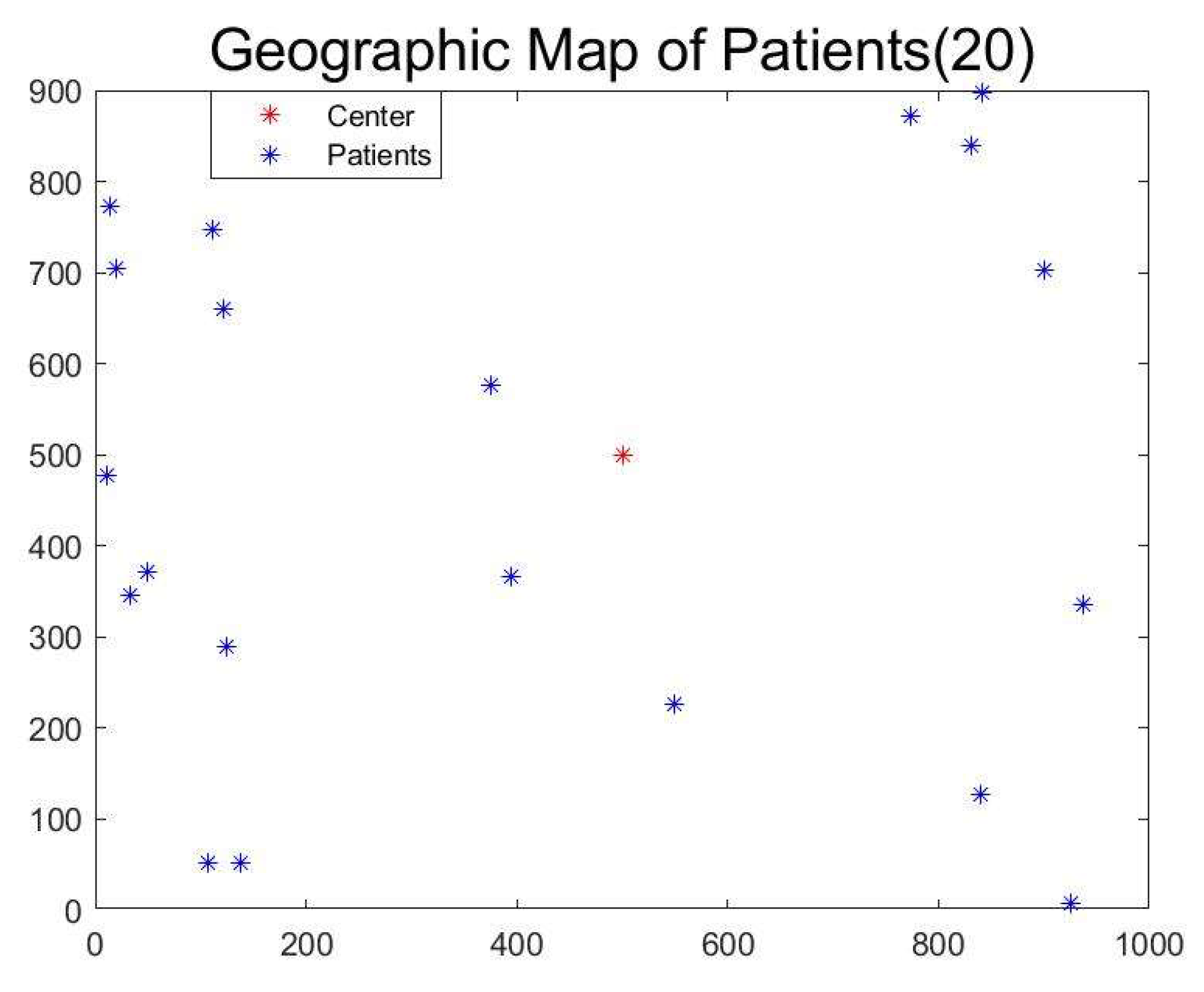
6.1. The Number of Patients Is 20

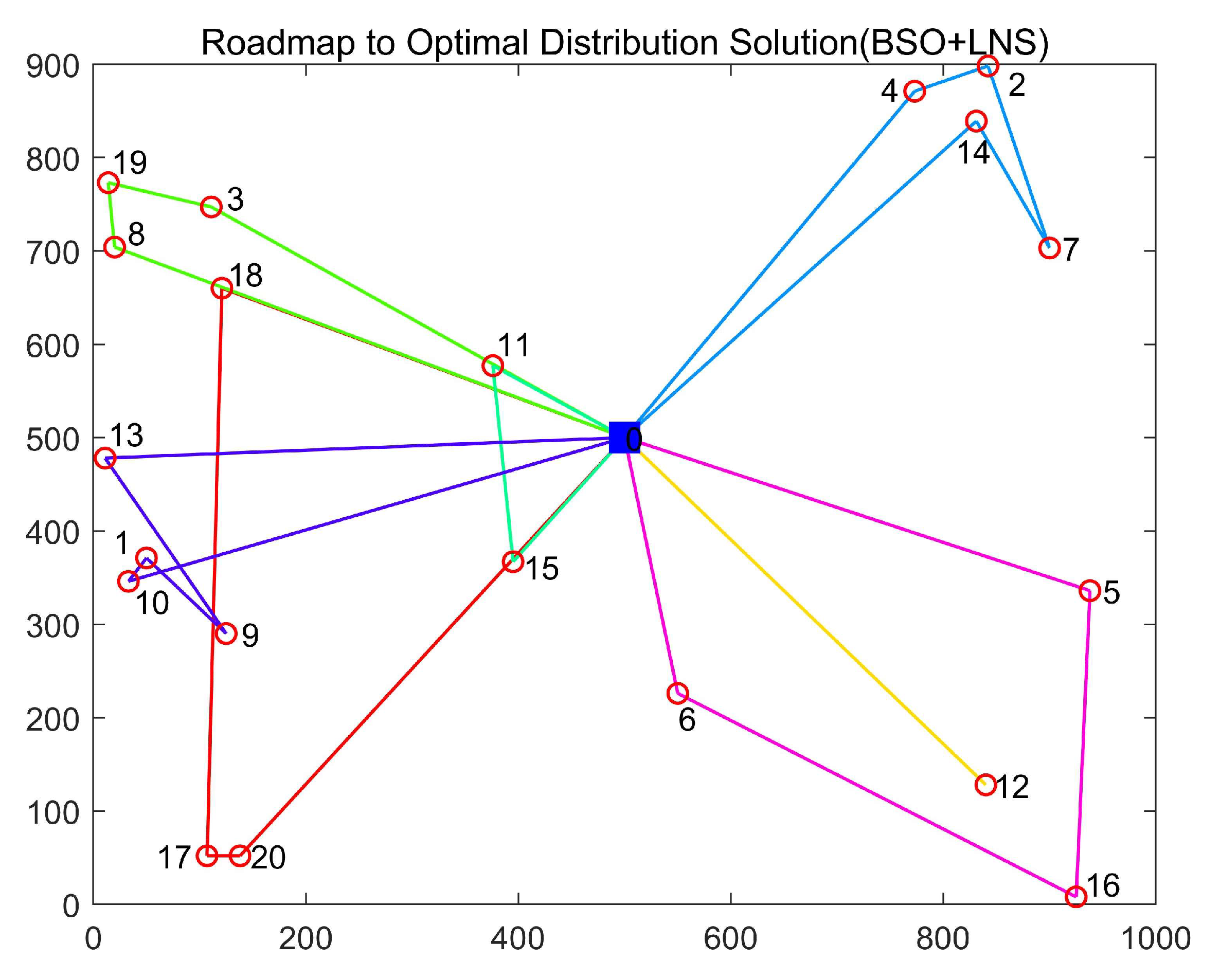
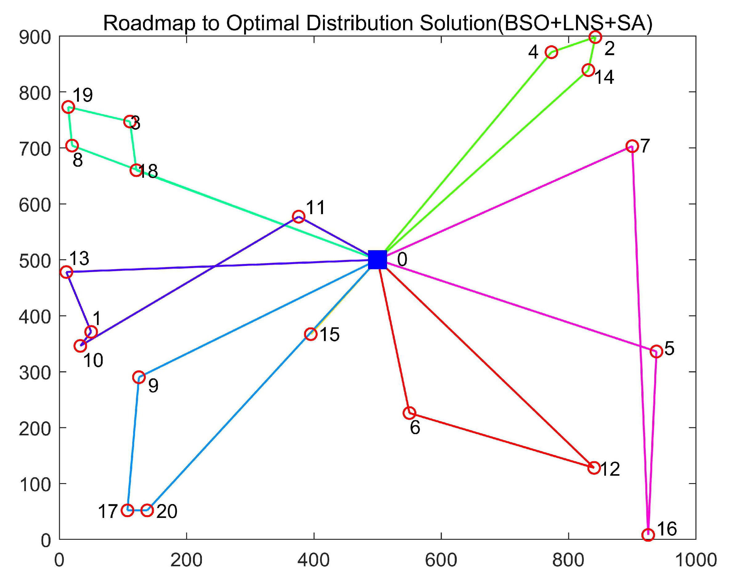
The initial location points of the 20 patients are shown in Figure 4. The maximum number of iterations is specified at 100. The BSO algorithm, BSO+LNS algorithm, and HBSO algorithm are applied to solve the model, respectively. After running three algorithms, roadmaps of the optimal relief solutions of the three algorithms are obtained, as shown in Figure 5, Figure 6 and Figure 7, respectively. The final results are shown in

Table 3. The final results from three algorithms.

	BSO	BSO+LNS	HBSO
Mean value of the objective function	40,107.8964	37,211.6867	37,069.2484
Variance of the objective function	1,000,988.112	160,159.8646	108,116.0327
Mean value of total travel distance	11,313.426	8455.6771	8313.2388
Variance of the total travel distance	942,419.6876	160,159.8646	108,116.0327
Final value of the deprivation cost	1894.5709	1892.0069	1892.0069

The bolded part of the table indicates the minimum value in the same row, i.e., the optimal value.

.

The experimental data show that the solution from the HBSO algorithm outperforms the other two methods in terms of overall performance when the number of patients is 20. The values of BSO+LNS and HBSO are significantly smaller than those of the original BSO in terms of the mean value of the objective function and the mean value of the total distance traveled. This shows that the LNS helps the algorithm to improve its ability to find the local optimal solution. Meanwhile, the variance of BSO+LNS and HBSO decreased more than 80% compared to the original BSO in terms of the variance of the objective function and the variance of the total distance traveled. It can be seen that LNS significantly improves the stability of the algorithm in finding the optimal solution. Comparing the metrics of HBSO and BSO+LNS, HBSO gets better results except for the value of the deprivation cost. It can be seen that the addition of SA also effectively improves the overall performance of the algorithm. In addition, in the variance of the objective function and the variance of the total distance traveled, HBSO is more than 30% more optimized than BSO+LNS, which can indicate that SA further helps the algorithm to improve its ability to jump out of the local optimum. For the mean value of the final deprivation cost, the results obtained by the three algorithms are not significantly different, indicating that the objective function is effectively established to prioritize relief for patients with more severe conditions.

6.2. The Number of Patients Is 30

The initial location points of the 30 patients are shown in Figure 8. The maximum number of iterations is specified at 200. The BSO algorithm, BSO+LNS algorithm, and HBSO algorithm are used to handle the model, respectively. The optimal relief solutions from the three algorithms are acquired when the number of patients is 30, as shown in Figure 9, Figure 10 and Figure 11, respectively. The final results are shown in

Table 4. The final results from three algorithms.

	BSO	BSO+LNS	HBSO
Mean value of the objective function	75,703.4705	66,433.5287	66,114.7729
Variance of the objective function	48,289,558.19	446,829.1021	204,987.2278
Mean value of total travel distance	16,826.8956	11,857.3197	11,548.8393
Variance of the total travel distance	1,574,368.618	483,280.751	185,060.18
Final value of the deprivation cost	5850.0669	5420.0303	5419.0027

The bolded part of the table indicates the minimum value in the same row, i.e., the optimal value.

.

When the number of patients is 30, the solution from the HBSO algorithm functions better than the other two methods. Comparing the results of the BSO algorithm with that of the BSO+LNS algorithm, it can be found that the LNS can significantly enhance the BSO algorithm’s performance. In particular, the BSO+LNS algorithm has greatly improved the variance of the objective function and the variance of the total travel distance. In the variance of the objective function, the BSO+LNS algorithm is two orders of magnitude smaller than the BSO algorithm. At the same time, in the variance of the total travel distance, the BSO+LNS algorithm is 70% smaller than the BSO algorithm. The outcomes indicate that the solutions of the algorithm could be more stable after adding the LNS. For the objective function and the total travel distance, the BSO+LNS algorithm also has a narrowing of more than 10%. Meanwhile, the BSO+LNS algorithm and the HBSO algorithm also show some advantages in terms of the deprivation cost. Similar to the previous experiment, all the findings of the HBSO algorithm outperform those of the BSO+LNS algorithm. Compared with BSO, the stability of BSO+LNS has been substantially improved. Furthermore, both variance metrics of HBSO have been reduced by more than 50% on top of BSO+LNS. This also proves that the SA algorithm could aid the algorithm in finding better solutions and having a more stable capability.

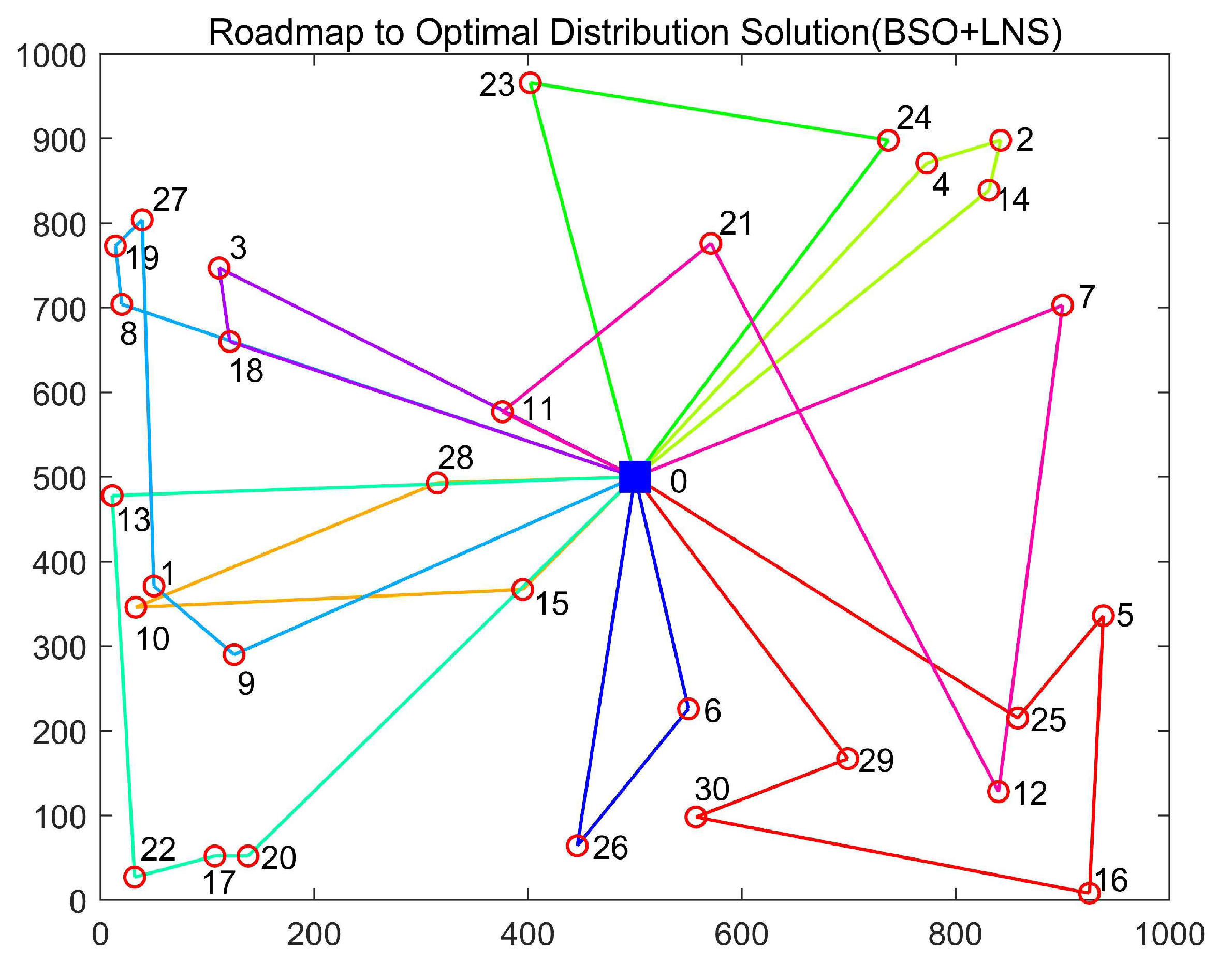
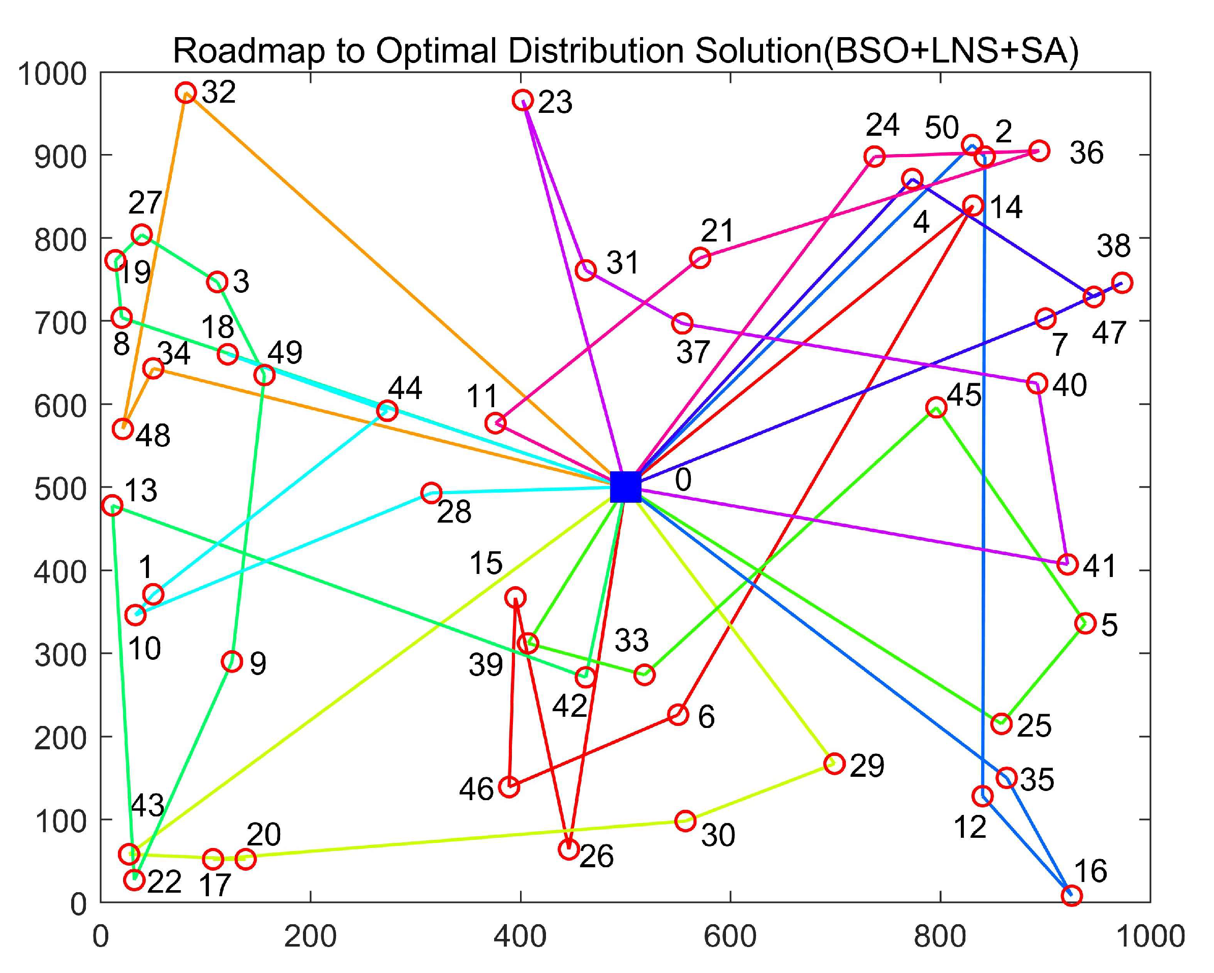
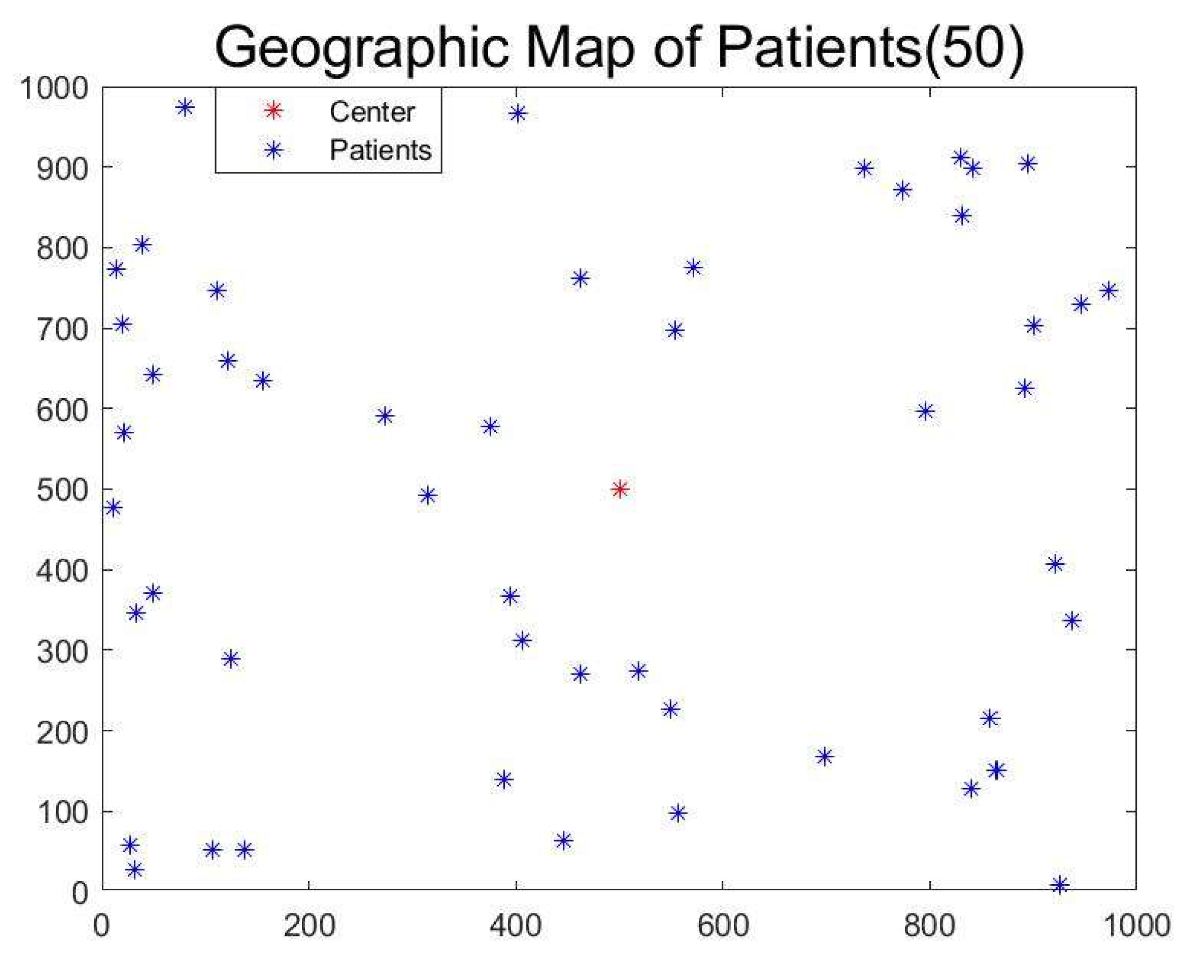
6.3. The Number of Patients Is 50

The initial location points of the 50 patients are shown in Figure 12. The maximum number of iterations is specified at 500. The BSO algorithm, BSO+LNS algorithm, and HBSO algorithm are utilized to solve the ERRP, and the optimal relief solutions of three algorithms are obtained when the number of patients is 50, as shown in Figure 13, Figure 14 and Figure 15, respectively. The final results are shown in

Table 5. The final results from three algorithms.

	BSO	BSO+LNS	HBSO
Mean value of the objective function	124,693.1177	54,772.0129	53,634.5471
Variance of the objective function	963,468,064.7578	5,631,143.023	6,982,170.224
Mean value of total travel distance	23,789.4376	18,100.1177	17,775.5003
Variance of the total travel distance	2,277,210.0198	1,621,395.4188	926,287.2734
Final value of the deprivation cost	24,717.2172	9069.8369	8870.4518

The bolded part of the table indicates the minimum value in the same row, i.e., the optimal value.

.

The HBSO algorithm also performs more comprehensively when the patient number is 50. On the five data in the results, the BSO+LNS algorithm and HBSO algorithm have a substantial reduction compared to the original BSO algorithm. On the mean of the objective function, HBSO and BSO+LNS are reduced by more than 50%. On the variance of the objective function, HBSO and BSO+LNS are even less than 1% of the original BSO. In terms of the mean and variance of the total distance traveled, HBSO and BSO+LNS have more than a 20% reduction. In particular, the final value of the deprivation cost of both decreases by more than 60%. Among them, the HBSO algorithm outperforms the BSO+LNS algorithm in four aspects: the mean value of the objective function, the mean value of the total travel distance, the variance of the total travel distance, and the final value of the deprivation cost. In the variance of the objective function, the HBSO algorithm shows a small increase. In general, the HBSO algorithm still has great advantages.

6.4. The Optimal Relief Solutions

In this section, we intercept the optimal solutions of the three algorithms with the smallest objective function values in 30 independent runs for analysis. The objective function values for the three sets of the total of nine results are plotted as histograms in Figure 16, and the data are presented in

Table 6. The optimal objective function values.

	BSO	BSO+LNS	HBSO
Objective function value (20)	145,10.0916	8479.3374	8213.7213
Objective function value (30)	21,105.4295	15,500.0604	15,906.6677
Objective function value (50)	79,521.7022	49,793.3165	49,137.4593

The bolded part of the table indicates the minimum value in the same row, i.e., the optimal value.

.

It can be found that the HBSO algorithm has been greatly improved over the original BSO algorithm for 20, 30, and 50 patients. This demonstrates the efficiency of the HBSO algorithm for solving the ERRP. Comparing the HBSO algorithm with the BSO+LNS algorithm, the results of HBSO are smaller for 20 and 50 patients. This indicates that the HBSO algorithm is able to find better solutions with the addition of the SA algorithm. The optimal solution of the HBSO algorithm is larger than the optimal solution of the BSO+LNS algorithm for a patient number of 30. Despite this, in chapter 5.2, we learn that the mean value of the objective function in 30 independent runs of the HBSO algorithm is less than that of the BSO+LNS. This shows that the HBSO algorithm is more stable than the BSO+LNS when solving the ERRP.

6.5. Discussion

After comparing the performance of HBSO, BSO+LNS, and the original BSO at patient numbers of 20, 30, and 50, the following conclusions were reached:

(1) Comparing the performance of BSO+LNS and the original BSO, it was observed that the addition of LNS significantly improved the convergence and stability of the algorithm. The neighborhood search behavior of LNS was found to be effective in finding optimal solutions, as evidenced by the decrease in the objective function value and total distance traveled. This improvement can be attributed to the local search operation performed during the iterative process of the BSO+LNS algorithm, which enhances the degree of exploitation and facilitates the identification of better individuals. The stability of BSO+LNS was also significantly improved, as evidenced by the two variance metrics. Furthermore, the deprivation cost was significantly optimized at patient number 50, which was not observed at patient numbers 20 and 30. As the number of patients increased, the algorithm with the addition of LNS exhibited superior optimization-seeking performance. These results confirm the effectiveness of incorporating LNS into BSO.

(2) The combined performance of HBSO was found to be superior to that of BSO+LNS, based on the results. At patient numbers 20 and 30, HBSO exhibited smaller variance, indicating greater stability in finding optimal solutions. HBSO only showed a slight optimization in the mean of the objective function and the mean of the total distance traveled. However, at a patient number of 50, HBSO exhibited more significant optimization than BSO+LNS in the mean value of the objective function, the mean value of the total distance traveled, and the deprivation cost. The analysis of the 30 results indicated that the HBSO algorithm with SA added possessed a stronger ability to find the optimal solution. The selective retention of non-optimal individuals according to the probability facilitated a deeper exploration of the solution space, resulting in a strong global search capability. However, HBSO exhibited a slight increase in the variance of the objective function at patient number 50 compared to BSO+LNS, possibly due to an imbalance in the relationship between LNS and SA. This will be addressed in future studies.

To demonstrate the efficacy of the model with the inclusion of the deprivation cost, the two models with and without the deprivation cost are compared. The objective functions with and without deprivation costs are used in three cases with patient numbers of 20, 30, and 50, respectively. The HBSO algorithm was then applied to solve the problem, each with 30 independent runs. After averaging the data, the results obtained were shown in

Table 7. The results of whether to include deprivation cost in the objective function.

The number of patients is 20	Deprivation cost 1	37,143.0729
	Deprivation cost 2	1892.0069
The number of patients is 30	Deprivation cost 3	60,618.7343
	Deprivation cost 4	5419.0027
The number of patients is 50	Deprivation cost 5	122,708.478
	Deprivation cost 6	8870.4518

and plotted as a bar chart in Figure 17, where deprivation cost 1, 3, and 5 are the distress levels of patients in the solutions when the number of patients is 20, 30, and 50, respectively, without adding the deprivation cost to the model. Deprivation cost 2, 4, and 6 are the distress levels of patients in the solutions when the model with deprivation cost is applied, respectively.

It is easy to tell from the figure that adding the deprivation cost to the model can significantly reduce the level of patients’ suffering. When the concept of deprivation cost is not introduced, although less costly solutions for distribution can be found, the patients will have to endure a greater amount of distress. This also shows that the traditional way of solving the VRP cannot be directly applied to the solution of the ERRP. The solution model that includes the deprivation cost is more in line with the fundamentals of providing humanitarian relief in post-disaster situations.

Algorithm complexity analysis is a crucial aspect of algorithm design and evaluation. In this study, we analyzed the time and space complexity of the proposed hybrid algorithm, which combines three different algorithms, namely BSO, LNS, and SA, to achieve superior performance. Our analysis reveals that there is no significant difference in complexity between BSO, BSO+LNS, and HBSO. Specifically, the time complexity of these algorithms is $O\left(n^2\right)$, and their space complexity is $O\left({log}_n\right)$.

In summary, our findings indicate a significant improvement in the synthesis ability of the HBSO algorithm as compared to the other two methods. The incorporation of LNS enhances the algorithm’s ability to exploit the solution space and discover superior individuals. By selectively retaining non-optimal individuals based on probability, the algorithm achieves a more comprehensive exploration of the solution space and a stronger global search capability. Additionally, our model, which incorporates deprivation cost, significantly reduces patient suffering, resulting in a higher likelihood of successful rescue and a more compassionate approach to healthcare.

7. Conclusions

In this paper, we introduce a novel approach for analyzing emergency relief routes that considers the well-being of patients by incorporating the deprivation costs of patients into the objective function. In addition, our model takes into account the total travel distance, penalties for violating time windows, and penalties for exceeding loading capacity. To optimize the model, we propose a new metaheuristic algorithm, HBSO, which integrates SA, LNS, and BSO algorithms. Simulation experiments are conducted to evaluate the effectiveness of the HBSO algorithm, which outperforms existing methods by achieving lower total cost (as reflected by smaller objective function values) and providing more stable solutions with smaller variances. Our study also demonstrates the feasibility of the BSO algorithm for solving route optimization problems. Importantly, our approach aims to alleviate the suffering of patients, which aligns with the humanitarian spirit of emergency relief.

The use of the BSO algorithm for optimizing vehicle routes has practical implications for material distribution in real-world scenarios. Moreover, the performance of the HBSO algorithm in the emergency relief routing model provides valuable insights for emergency relief actions. Our proposed HBSO algorithm effectively enhances the performance of the BSO algorithm in emergency relief problems by integrating LNS and SA selection steps, enabling the algorithm to obtain superior solutions and avoid local optima. Future research could explore the application of HBSO algorithms to other disaster management problems, such as resource allocation and emergency evacuation planning, or adapt the algorithms to solve optimization problems in other domains, such as transportation or logistics. In addition, future research could investigate the performance of HBSO algorithms on larger scale problems or on different types of input data. However, it should be noted that obtaining accurate patient location information in real-life emergency relief operations may not always be feasible, as opposed to the simulation experiments presented in this study. Therefore, developing an efficient method for rapidly updating relief routes as patient locations change in real-time is a critical research topic that warrants further investigation. In our future research, we plan to focus on developing a method that can effectively and efficiently update relief routes in response to changing patient location information to improve the timeliness and effectiveness of emergency relief operations.

References

1. Huang, M.; Smilowitz, K.; Balcik, B. Models for relief routing: Equity, efficiency and efficacy. Transp. Res. Part E Logist. Transp. Rev. 2012, 48, 2–18. [Google Scholar] [CrossRef]
2. Tavakkoli-Moghaddam, R.; Shishegar, S.; Siadat, A.; Mohammadi, M. Design of a Reliable Bi-objective Relief Routing Network in the Earthquake Response Phase. Procedia Comput. Sci. 2016, 102, 74–81. [Google Scholar] [CrossRef]
3. Wei, X.; Qiu, H.; Wang, D.; Duan, J.; Wang, Y.; Cheng, T.C.E. An integrated location-routing problem with post-disaster relief distribution. Comput. Ind. Eng. 2020, 147, 106632. [Google Scholar] [CrossRef]
4. Huang, M.; Smilowitz, K.R.; Balcik, B. A continuous approximation approach for assessment routing in disaster relief. Transp. Res. Part B Methodol. 2013, 50, 20–41. [Google Scholar] [CrossRef]
5. Nadi, A.; Edrisi, A. Adaptive multi-agent relief assessment and emergency response. Int. J. Disaster Risk Reduct. 2017, 24, 12–23. [Google Scholar] [CrossRef]
6. Kirac, E.; Milburn, A.B. A general framework for assessing the value of social data for disaster response logistics planning. Eur. J. Oper. Res. 2018, 269, 486–500. [Google Scholar] [CrossRef]
7. Maya Duque, P.A.; Dolinskaya, I.S.; Sörensen, K. Network repair crew scheduling and routing for emergency relief distribution problem. Eur. J. Oper. Res. 2016, 248, 272–285. [Google Scholar] [CrossRef]
8. Macone, D.; Oddi, G.; Pietrabissa, A. MQ-Routing: Mobility-, GPS- and energy-aware routing protocol in MANETs for disaster relief scenarios. Ad Hoc Netw. 2013, 11, 861–878. [Google Scholar] [CrossRef]
9. Beamon, B.M.; Balcik, B. Performance measurement in humanitarian relief chains. Int. J. Public Sect. Manag. 2008, 21, 4–25. [Google Scholar] [CrossRef]
10. Holguín-Veras, J.; Jaller, M.; Van Wassenhove, L.N.; Pérez, N.; Wachtendorf, T. On the unique features of post-disaster humanitarian logistics. J. Oper. Manag. 2012, 30, 494–506. [Google Scholar] [CrossRef]
11. Sabouhi, F.; Bozorgi-Amiri, A.; Moshref-Javadi, M.; Heydari, M. An integrated routing and scheduling model for evacuation and commodity distribution in large-scale disaster relief operations: A case study. Ann. Oper. Res. 2019, 283, 643–677. [Google Scholar] [CrossRef]
12. Holguín-Veras, J.; Pérez, N.; Jaller, M.; Van Wassenhove, L.N.; Aros-Vera, F. On the appropriate objective function for post-disaster humanitarian logistics models. J. Oper. Manag. 2013, 31, 262–280. [Google Scholar] [CrossRef]
13. Shi, Y. Brain Storm Optimization Algorithm. In Advances in Swarm Intelligence, Proceedings of the International Conference on Swarm Intelligence 2011, Chongqing, China, 12–15 June 2011; Tan, Y., Shi, Y., Chai, Y., Wang, G., Eds.; Springer: Berlin/Heidelberg, Germany, 2011; pp. 303–309. [Google Scholar]
14. Beibei, S.; Hua, Y.; Asghar, H.A.; Long, Z.; Zhongyi, H.; Huiling, C.; Hamza, T.; Majdi, M.; Peiliang, W. Analysis of COVID-19 severity from the perspective of coagulation index using evolutionary machine learning with enhanced brain storm optimization. J. King Saud Univ. Comput. Inf. Sci. 2022, 34, 4874–4887. [Google Scholar]
15. Timea, B.; Miodrag, Z.; Nebojsa, B.; Amit, C.; Muthusamy, S. Feature Selection by Hybrid Brain Storm Optimization Algorithm for COVID-19 Classification. J. Comput. Biol. A J. Comput. Mol. Cell Biol. 2022, 29, 515–529. [Google Scholar]
16. Fahim, A.; Abdelraheem, N. An Adaptive Discrete Brain Storm Algorithm Solves 3D Protein Structure Prediction. Int. J. Adv. Comput. Sci. Appl. (IJACSA) 2021, 12, 850–858. [Google Scholar] [CrossRef]
17. Yang, J.; Shen, Y.; Shi, Y. Visual fixation prediction with incomplete attention map based on brain storm optimization. Appl. Soft Comput. J. 2020, 96, 106653. [Google Scholar] [CrossRef]
18. Alzaqebah, M.; Jawarneh, S.; Alwohaibi, M.; Alsmadi, M.K.; Almarashdeh, I.; Mohammad, R.M. Hybrid Brain Storm Optimization Algorithm and Late Acceptance Hill Climbing to solve the Flexible Job-Shop Scheduling Problem. J. King Saud Univ. Comput. Inf. Sci. 2020, 34, 2926–2937. [Google Scholar] [CrossRef]
19. Narmatha, C.; Eljack, S.M.; Tuka, A.A.R.M.; Manimurugan, S.; Mustafa, M. A hybrid fuzzy brain-storm optimization algorithm for the classification of brain tumor MRI images. J. Ambient Intell. Humaniz. Comput. 2020. [Google Scholar] [CrossRef]
20. Aldhafeeri, A.; Rahmat-Samii, Y. Brain Storm Optimization for Electromagnetic Applications: Continuous and Discrete. IEEE Trans. Antennas Propag. 2019, 67, 2710–2722. [Google Scholar] [CrossRef]
21. Xingsi, X. Complex ontology alignment for autonomous systems via the Compact Co-Evolutionary Brain Storm Optimization algorithm. ISA Trans. 2022, 132, 190–198. [Google Scholar]
22. Zonghui, C.; Shangce, G.; Xiao, Y.; Gang, Y.; Shi, C.; Yuhui, S. Alternate search pattern-based brain storm optimization. Knowl. Based Syst. 2022, 238, 107896. [Google Scholar]
23. Zhao, F.; Hu, X.; Wang, L.; Zhao, J.; Tang, J. A reinforcement learning brain storm optimization algorithm (BSO) with learning mechanism. Knowl. Based Syst. 2022, 235, 107645. [Google Scholar] [CrossRef]
24. Wei, L.; Haonan, L.; Lei, W.; Qiaoyong, J.; Qingzheng, X. Enhanced Brain Storm Optimization Algorithm Based on Modified Nelder–Mead and Elite Learning Mechanism. Mathematics 2022, 10, 1303. [Google Scholar]
25. Ma, L.; Cheng, S.; Shi, Y. Enhancing Learning Efficiency of Brain Storm Optimization via Orthogonal Learning Design. IEEE Trans. Syst. Man Cybern. Syst. 2021, 51, 6723–6742. [Google Scholar] [CrossRef]
26. Jia, Z.; Duan, H.; Shi, Y. Hybrid brain storm optimisation and simulated annealing algorithm for continuous optimisation problems. Int. J. Bio-Inspired Comput. 2016, 8, 109–121. [Google Scholar] [CrossRef]
27. Shaw, P. Using Constraint Programming and Local Search Methods to Solve Vehicle Routing Problems. In Proceedings of the Principles and Practice of Constraint Programming—CP98, 1998 International Conference on Principles and Practice of Constraint Programming (CP’98), Pisa, Italy, 26–30 October 1998; Maher, M., Puget, J.-F., Eds.; Springer: Berlin/Heidelberg, Germany, 1998; pp. 417–431. [Google Scholar]
28. Pisinger, D.; Ropke, S. Large Neighborhood Search. In Handbook of Metaheuristics; Gendreau, M., Potvin, J.-Y., Eds.; Springer International Publishing: Cham, Switzerland, 2019; pp. 99–127. [Google Scholar]
29. Goeke, D.; Roberti, R.; Schneider, M. Exact and Heuristic Solution of the Consistent Vehicle-Routing Problem. Transp. Sci. 2019, 53, 1023–1042. [Google Scholar] [CrossRef]
30. Fadda, P.; Mancini, S.; Serra, P.; Fancello, G. The Heterogeneous Fleet Vehicle Routing Problem with Draft Limits. Comput. Oper. Res. 2023, 149, 106024. [Google Scholar] [CrossRef]
31. Eskandarpour, M.; Ouelhadj, D.; Hatami, S.; Juan, A.A.; Khosravi, B. Enhanced multi-directional local search for the bi-objective heterogeneous vehicle routing problem with multiple driving ranges. Eur. J. Oper. Res. 2019, 277, 479–491. [Google Scholar] [CrossRef]
32. Metropolis, N.; Rosenbluth, A.; Rosenbluth, M.; Teller, A.; Teller, E. Simulated annealing. J. Chem. Phys. 1953, 21, 1087–1092. [Google Scholar] [CrossRef]
33. İLhan, İ. An improved simulated annealing algorithm with crossover operator for capacitated vehicle routing problem. Swarm Evol. Comput. 2021, 64, 100911. [Google Scholar] [CrossRef]
34. Yu, V.F.; Jewpanya, P.; Redi, A.A.N.P.; Tsao, Y.-C. Adaptive neighborhood simulated annealing for the heterogeneous fleet vehicle routing problem with multiple cross-docks. Comput. Oper. Res. 2021, 129, 105205. [Google Scholar] [CrossRef]
35. Oruc, B.E.; Kara, B.Y. Post-disaster assessment routing problem. Transp. Res. Part B 2018, 116, 76–102. [Google Scholar] [CrossRef]
36. Berktaş, N.; Kara, B.; Karaşan, O. Solution methodologies for debris removal in disaster response. EURO J. Comput. Optim. 2016, 4, 403–445. [Google Scholar] [CrossRef]
37. Masaracchia, A.; Nguyen, L.D.; Duong, T.Q.; Nguyen, M.N. An Energy-Efficient Clustering and Routing Framework for Disaster Relief Network. IEEE Access 2019, 7, 56520–56532. [Google Scholar] [CrossRef]
38. Song, F.; Ma, Y.; You, I.; Zhang, H. Smart Collaborative Evolvement for Virtual Group Creation in Customized Industrial IoT. IEEE Trans. Netw. Sci. Eng. 2022, 1–11. [Google Scholar] [CrossRef]
39. Stute, M.; Kohnhäuser, F.; Baumgärtner, L.; Almon, L.; Hollick, M.; Katzenbeisser, S.; Freisleben, B. RESCUE: A Resilient and Secure Device-to-Device Communication Framework for Emergencies. IEEE Trans. Dependable Secur. Comput. 2022, 19, 1722–1734. [Google Scholar] [CrossRef]
40. Campbell, A.M.; Vandenbussche, D.; Hermann, W. Routing for Relief Efforts. Transp. Sci. 2008, 42, 127–145. [Google Scholar] [CrossRef]
41. Nair, D.J.; Rey, D.; Dixit, V.V. Fair allocation and cost-effective routing models for food rescue and redistribution. IISE Trans. 2017, 49, 1172–1188. [Google Scholar] [CrossRef]
42. Özdamar, L.; Demir, O. A hierarchical clustering and routing procedure for large scale disaster relief logistics planning. Transp. Res. Part E Logist. Transp. Rev. 2012, 48, 591–602. [Google Scholar] [CrossRef]
43. Rath, S.; Gutjahr, W.J. A math-heuristic for the warehouse location–routing problem in disaster relief. Comput. Oper. Res. 2014, 42, 25–39. [Google Scholar] [CrossRef]
44. Goli, A.; Malmir, B. A Covering Tour Approach for Disaster Relief Locating and Routing with Fuzzy Demand. Int. J. Intell. Transp. Syst. Res. 2020, 18, 140–152. [Google Scholar] [CrossRef]
45. Ozdamar, L.; Aksu, D.T.; Yasa, E.; Ergunes, B. Disaster relief routing in limited capacity road networks with heterogeneous flows. J. Ind. Manag. Optim. 2018, 14, 1367. [Google Scholar] [CrossRef]
46. Al Theeb, N.; Murray, C. Vehicle routing and resource distribution in postdisaster humanitarian relief operations. Int. Trans. Oper. Res. 2017, 24, 1253–1284. [Google Scholar] [CrossRef]
47. Bruni, M.E.; Beraldi, P.; Khodaparasti, S. A fast heuristic for routing in post-disaster humanitarian relief logistics. Transp. Res. Procedia 2018, 30, 304–313. [Google Scholar] [CrossRef]
48. Li, Y.; Chung, S.H. Disaster relief routing under uncertainty: A robust optimization approach. IISE Trans. 2019, 51, 869–886. [Google Scholar] [CrossRef]
49. Wang, H.; Du, L.; Ma, S. Multi-objective open location-routing model with split delivery for optimized relief distribution in post-earthquake. Transp. Res. Part E Logist. Transp. Rev. 2014, 69, 160–179. [Google Scholar] [CrossRef]
50. Alinaghian, M.; Aghaie, M.; Sabbagh, M.S. A mathematical model for location of temporary relief centers and dynamic routing of aerial rescue vehicles. Comput. Ind. Eng. 2019, 131, 227–241. [Google Scholar] [CrossRef]
51. Çankaya, E.; Ekici, A.; Özener, O.Ö. Humanitarian relief supplies distribution: An application of inventory routing problem. Ann. Oper. Res. 2019, 283, 119–141. [Google Scholar] [CrossRef]
52. Nasiri, M.M.; Shishegar, S. Disaster relief routing by considering heterogeneous vehicles and reliability of routes using an MADM approach. Uncertain Supply Chain Manag. 2014, 2, 137–150. [Google Scholar] [CrossRef]
53. Sakiani, R.; Seifi, A.; Khorshiddoust, R.R. Inventory routing and dynamic redistribution of relief goods in post-disaster operations. Comput. Ind. Eng. 2020, 140, 106219. [Google Scholar] [CrossRef]
Figure 1. The constant penalty and deprivation cost.
Sustainability 15 08187 g001
Figure 2. The flowchart of the BSO algorithm.
Sustainability 15 08187 g002
Figure 3. The flowchart of the ERRP solving model based on the HBSO.
Sustainability 15 08187 g003
Figure 4. The location of patients (20).
Sustainability 15 08187 g004
Figure 5. The optimal relief route from the BSO algorithm (20).
Sustainability 15 08187 g005
Figure 6. The optimal relief route from the BSO+LNS algorithm (20).
Sustainability 15 08187 g006
Figure 7. The optimal relief route from the HBSO algorithm (20).
Sustainability 15 08187 g007
Figure 8. The location of patients (30).
Sustainability 15 08187 g008
Figure 9. The optimal relief route from the BSO algorithm (30).
Sustainability 15 08187 g009
Figure 10. The optimal relief route from the BSO+LNS algorithm (30).
Sustainability 15 08187 g010
Figure 11. The optimal relief route from the HBSO algorithm (30).
Sustainability 15 08187 g011
Figure 12. The location of patients (50).
Sustainability 15 08187 g012
Figure 13. The optimal relief route from the BSO algorithm (50).
Sustainability 15 08187 g013
Figure 14. The optimal relief route from the BSO+LNS algorithm (50).
Sustainability 15 08187 g014
Figure 15. The optimal relief route from the HBSO algorithm (50).
Sustainability 15 08187 g015
Figure 16. The optimal objective function values.
Sustainability 15 08187 g016
Figure 17. Comparison of whether to include deprivation cost in the objective function.
Sustainability 15 08187 g017