Article

Machine Learning Supervisory Control of Grid-Forming Inverters in Islanded Mode

by
Hammed Olabisi Omotoso
1,
Abdullrahman A. Al-Shamma’a
2,
Mohammed Alharbi
1,*,
Hassan M. Hussein Farh
2,
Abdulaziz Alkuhayli
1,
Akram M. Abdurraqeeb
1,
Faisal Alsaif
1,
Umar Bawah
1 and
Khaled E. Addoweesh
1
1
Department of Electrical Engineering, College of Engineering, King Saud University, Riyadh 11421, Saudi Arabia
2
Department of Electrical Engineering, College of Engineering, Imam Mohammad Ibn Saud Islamic University, Riyadh 11432, Saudi Arabia
*
Author to whom correspondence should be addressed.
Sustainability 2023, 15(10), 8018; https://doi.org/10.3390/su15108018
Submission received: 9 April 2023 / Revised: 8 May 2023 / Accepted: 12 May 2023 / Published: 15 May 2023
(This article belongs to the Special Issue Smart Grid Technologies and Renewable Energy Applications)

Abstract

:
This research paper presents a novel droop control strategy for sharing the load among three independent converter power systems in a microgrid. The proposed method employs a machine learning algorithm based on regression trees to regulate both the system frequency and terminal voltage at the point of common coupling (PCC). The aim is to ensure seamless transitions between different modes of operation and maintain the load demand while distributing it among the available sources. To validate the performance of the proposed approach, the paper compares it to a traditional proportional integral (PI) controller for controlling the dynamic response of the frequency and voltage at the PCC. The simulation experiments conducted in MATLAB/Simulink show the effectiveness of the regression tree machine learning algorithm over the PI controller, in terms of the step response and harmonic distortion of the system. The results of the study demonstrate that the proposed approach offers an improved stability and efficiency for the system, making it a promising solution for microgrid operations.

1. Introduction

The increasing demand for electricity, coupled with the pressing concerns of global warming, have prompted a substantial increase in the use of renewable energy resources such as photovoltaic (PV) and wind energy. The integration of such resources has accelerated the development of microgrids, which represent a form of distributed energy sources [1,2,3]. A microgrid is essentially a connected unit of the grid, consisting of one or more distributed generation (DG) units in proximity that can operate either in parallel with or independently of a power utility grid, while providing reliable power to various consumers.
The high integration of renewable energy sources poses challenges for power system operations [4,5]. Although PV/Wind integrated into an MG system have irrefutably brought positive impacts such as voltage regulation, line loss reduction, frequency regulation, and a reduction in distribution and transmission congestion [6], they still suffer from serious setbacks. In particular, their failure to ensure a continuous energy supply because their erratic and unstable nature impacts the grid integration. Therefore, voltage and frequency regulation are vital if the appropriate voltage and frequency at the customer’s point of common coupling (PCC) are to be sustained [7].
Inverters serve as a crucial component for the operation of microgrids in both islanded and grid-connected modes. In grid-connected systems, the grid regulates the voltage and frequency, rendering the inverters as grid-following inverters [8]. Conversely, a grid-forming inverter actively shapes the grid by controlling its output voltage and frequency, in contrast to a grid-following inverter that simply adjusts its output to align with the existing grid conditions [9]. This approach enables the grid to maintain stability, even during times of high demand or sudden changes in the grid conditions.
Numerous techniques have been adopted to validate the importance of using grid-connected inverters for power factor (PF), voltage, and reactive power control at the PCC [10]. The process can be achieved by regulating the power flow between the PV/wind sources and at the PCC. Conversely, the utilization of a grid-connected inverter to render ancillary services is very difficult. The high R/X ratio in the LV/MV of grid-connected inverters and the AC bus is ineligible because of the transmission line impedance [11]. This impedance creates system uncertainty. The instability of grid-connected inverters, especially in the presence of fluctuating grid impedance and weak grid conditions, is a major detrimental consequence of utilizing a PV/Wind system [12]. Another effect is the coupling between the reactive and active power flows [13], which is detrimental to both the grid voltage and frequency. Another disadvantage of complicated line impedance is that it has a direct impact on power factor (PF) control [14,15]. For instance, when the inverter’s power references are adjusted to only introduce active power, a unity PF is obtained at the output. Contrarily, the PF will differ at the grid side because of the reactive power, which compensates for reactive losses across the line impedance. These series of predicaments can be ameliorated using GFMIs, as this will proffer a favorable solution by reinforcing the grid. The regulation of the voltage and frequency of the grid is a primary objective of GFMIs [16]. In GFMIs, the converters are robustly synchronized to the grid with a proactive control mechanism in fault situations to maintain both the frequency and voltage stability [17,18]. These are essential for the high penetration of renewable energy resources in the islanded mode, weak grids, and decentralized power systems [19].
One key aspect of GFMI operations is the need for proper supervisory control [20] to ensure that the inverter behaves as desired. One common approach to supervisory control is the use of a PI controller, which is a type of feedback controller that uses the error between the desired and actual output to adjust the control signal. Studies have shown that PI controllers can effectively control GFMIs in a few different scenarios. A PI controller was used for the local voltage of a distributed system in [21]. The results showed that the PI controller was able to effectively track the desired power output and maintain the stable operation of the system. Sharma et al. [22] developed an approach using a PI controller for the seamless transition of incoming inverters in a GFMI. A fuzzy logic controller (FLC) is presented in [23] for the supervisory control of an islanded AC microgrid. The performance of the FLC produced a superior result when compared to a PI controller.
Several considerations should be considered when designing a PI controller for GFMI control. One important factor is the gain parameters of the controller [24,25], which determine the strength of the control signal. If the gain is too low, the controller may be slow to respond to changes in the system, whereas if the gain is too high, the controller may produce unstable oscillations. The proper tuning of the gain parameters is therefore critical for achieving the optimal performance. In [26], the authors analyzed the effects of different gain parameters on the performance of a PI controller. The results showed that the optimal gain parameters varied depending on the system’s operating conditions and that proper tuning was crucial for achieving a good performance. While traditional feedback controllers, such as PI controllers, have been widely used for GFMI control, few studies have focused on the use of machine learning algorithms for this GFMI control. A regression tree algorithm is presented in this study for the supervisory control of a GFMI. In contrast to PI controllers, which are based on a fixed set of gain parameters and must be properly tuned for optimal performance, regression trees have the capability to learn from data and adapt to changes in a system, which may make them more robust in the face of changing operating conditions.
The main objective of this study is to propose a droop control method for load sharing among three autonomous converter power systems in a microgrid and to ensure smooth transitions between different modes of operation, while maintaining the load demand and distributing it among the available sources. The proposed approach utilizes a regression tree machine learning algorithm to regulate both the system frequency and terminal voltage at the point of common coupling (PCC). The study demonstrates the efficacy of the regression tree machine learning algorithm over the traditional PI controller in terms of the step response and harmonic distortion, leading to an improved stability and efficiency for the system.
The study’s contribution is evident in the following aspects:
Firstly, the paper introduces the use of a regression tree machine learning algorithm to regulate the system frequency and terminal voltage, a novel approach for microgrid operations. Secondly, the paper presents a comprehensive evaluation of the proposed approach, including comparisons with a traditional PI controller, a step response analysis, and a harmonic distortion analysis. Finally, the study demonstrates the effectiveness of the proposed approach in achieving a stable frequency and voltage operation, as well as meeting the IEEE 519 power harmonic standards.
The remaining parts of the paper are as follows: Section 2 describes the regression tree algorithm and studied system. Section 3 illustrates the regression tree algorithm, datasets, and data preprocessing. Section 4 discusses the simulation results. Section 5 presents the conclusion.

2. System Modelling and Configuration

Figure 1 illustrates a schematic diagram of the proposed microgrid. The entire system is self-reliant. The microgrid is made up of three DG units with a single local load unit connected to the three DG units at the PCC. A linear RL load and nonlinear load, which is related to the voltage magnitude and frequency, are employed. The input sources are considered to have a sufficient capacity to supply the loads, and the entire loads are shared by both converters in accordance with their capacities.

2.1. Dynamic Model

Each DG unit has its own local frequency that is monitored via a phase-locked loop (PLL) by allocating a drop converter to each converter to share the total load. The system’s dynamic equations are expressed as follows:
V s x = V m x L s x h I s x R s x I s x = M x V d c x 2 , h = d d t   a n d   x = 1 , 2 n .
where V s x , M x   , and   I s x are the output phase voltage, modulation index, and phase current of the converter, respectively. V m x , L s x , and R s x , are the load voltage, transmission line inductance, and resistance of D G x respectively.
The voltage equation for the linear loads is introduced by:
V m x = R L x I L x + L L x h I L x
where I L x , R L x , and L L x are the phase current, resistance, and inductance of the linear load, respectively.
The nonlinear load is represented as:
P x N o n = P x 0 V m x V n 2 f s x f n 2
Q x N o n = Q x 0 V m x V n 2 f s x f n 2
where P x N o n and Q x N o n are the base active and reactive powers of the nonlinear loads, respectively. V m x and f s x are the local load voltage magnitude and frequency, respectively. f n and V n are the nominal voltage and frequency of the system, respectively.
A synchronous reference frame (SRF) is available for individual converter local frequency control. This is used to transform the dynamic equation of the model into a direct-quadrature ( q d ) reference frame to generate time-invariant variables.
The q d reference frame dynamic equations are represented as:
V s x q = V m x q L s x h I s x q R s x I s x q w s x L s x I s x d = M x q V d c x 2
V s x d = V m x d L s x h I s x d R s x I s x d + w s x L s x I s x q = M x d V d c x 2
The linear load voltage equation is represented as:
V m x q = R L x I L x q + L L x h I L x q + w s x L L x I L x d
V m x d = R L x I L x d + L L x h I L x d w s x L L x I L x q
For the nonlinear load current equation:
I x N o n q = 2 3 P x N o n V m x q Q x N o n V m x d V m x q 2 + V m x d 2
I x N o n d = 2 3 P x N o n V m x d + Q x N o n V m x q V m x q 2 + V m x d 2
For the constant load current equation:
I x q = 2 3 P x V m x q Q x V m x d V m x q 2 + V m x d 2
I x d = 2 3 P x V m x d + Q x V m x q V m x q 2 + V m x d 2

2.2. Control Unit

Because the micro-grid is self-contained, the voltage magnitude and frequency of each DG unit should be established in addition to feeding the overall load. Each converter’s control unit, as shown in Figure 2, is made up of four basic parts: a droop control to divide the load across the converters, a voltage control, and an inner current control. To align the load voltage in the q axis reference frame and monitor the local frequency, a phase-locked loop (PLL) is implemented.

2.2.1. Droop Control

The droop control approach is utilized in traditional power plant generators. This technology may be used in the independent operation of converter-based DG systems to share the total load while also managing the voltage magnitude and frequency in a certain range [27].
The active power of the overall load can be shared in this control unit by drooping the frequency as a function of the converter’s output active power. Furthermore, to share the total load reactive power, one can droop the converter’s output voltage magnitude against its output reactive power. Two coefficients regulate the slope of change in the voltage and frequency versus the active and reactive power, as illustrated in (13) and (14).
V m x * = V n n q x Q s x
ω x * = ω n m p x P s x
where V n , w n , m p x ,   n q x , P s x ,     and   Q s x   are the rated voltage, rated frequency, active power droop coefficients, reactive power droop coefficient, output active power, and output reactive power of the converter, respectively.
The quantity of the droop coefficients is specified in (15) and (16). The active power droop coefficient is calculated by comparing the maximum change in the frequency, which is 1%, to the maximum change in the active power, which equals the converter’s nominal power.
n q x = Δ V Δ Q s m   m a x
m p x = Δ ω Δ P s m   m a x
The maximum voltage tolerance is limited to 4% for the reactive power droop coefficient. Therefore, to have a similar frequency in the system,
w n m p 1 P s 1 = w n m p 2 P s 2
m p 1 m p 2 = P s 2 P s 1
This indicates that if the second converter’s nominal power is twice that of the first, the second converter’s active power droop coefficient should be half that of the first.
Figure 3 illustrates the droop control unit in detail. Initially, the converter’s instantaneous active and reactive power are estimated by monitoring the converter’s output current and load voltage.
P ˜ s x = 3 2 V m x q I s x q + V m x d I s x d
Q ˜ s x = 3 2 V m x q I s x d V m x d I s x q
The calculated instantaneous active and reactive power are sent through a low-pass filter with a cut of frequency of w c , which is roughly 10% of the nominal frequency, to eliminate fluctuations and obtain the average values of the output powers.
P s x = w c s + w c P ˜ s x
Q s x = w c s + w c Q ˜ s x
The voltage magnitude and angular frequency are outputs of the droop control. These are used to establish the reference angle of the load voltage using an integrator. As a result, the q d axis reference voltage may be calculated as follows:
V m x q * = V m x * cos ( θ x * θ s x )
V m x d * = V m x * sin ( θ x * θ s x )
Where θ s w is the transformation angle of the q d axis reference frame. This angle is the local frequency of each converter in this article, which is the PLL’s output.

2.2.2. Voltage Control

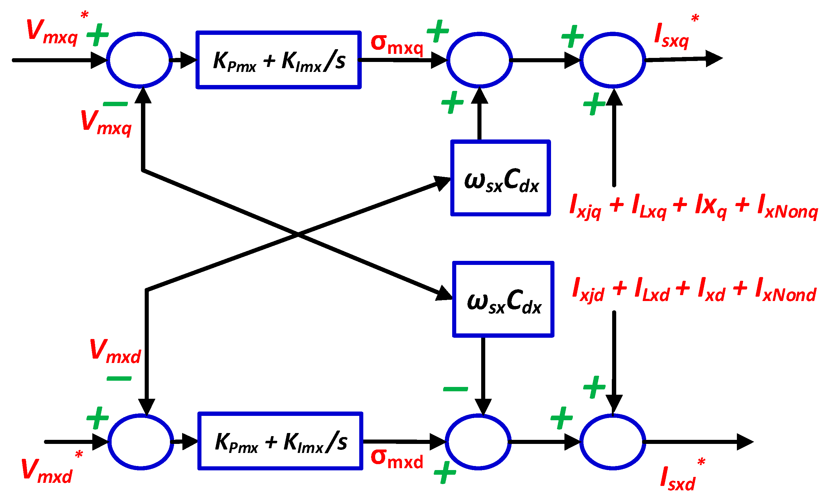
The PI voltage controller is meant to follow the load reference voltage created through the droop control. As shown in Figure 4, according to Equations (13) and (14), the system’s dynamic equations in Laplace format are:
C k x h V m x q = I s x q I x j q I L x q I x q I x N o n q w s x C k x V m x d
C k x h V m x d = I s x d I x j d I L x d I x d I x N o n d + w s x C k x V m x q
C k x h V m x q = k m x q s ( V m x q * V m x q ) = σ m x q
C k x h V m x q = k m x d s ( V m x d * V m x d ) = σ m x d
The PI voltage controllers are represented as:
k m x q s = k m x d s = k P m x + K I m x s
The voltage control transfer function can be obtained by substituting (29) into (27) and (28) and comparing it to a normal first-order transfer function with a time constant of τ m x , as:
V m x q V m x q * = k m x q s s C k x k m x q s = 1 1 + τ m x S = 1 1 + s C k x k m x q s
V m x d V m x d * = k m x d s s C k x k m x d s = 1 1 + τ m x S = 1 1 + s C k x k m x d s
As a result, upon using the controller’s time constant and the capacitance of the load capacitor, the PI controller parameters may be computed as follows:
k m x q s = k m x q s = s C k x s τ m x = k P m x + K I m x s
k P m x = C k x τ m x a n d   K I m x = 0
A small-time constant is required for a quick voltage control response; however, it should not be so tiny that it is less than the switching time interval. As a result, it is set to be around 10 times the switching time interval, as follows:
τ m x = 10 2 π f s w x
where the switching frequency of the converter for the D G x is f s w x .
I s x q * = σ m x q + I x j q + I L x q + I x q + I x N o n q + w s x C k x V m x d
I s x d * = σ m x d + I x j d + I L x d + I x d + I x N o n d w s x C k x V m x d
where σ m x q and σ m x d are the PI controllers’ output voltages.

2.2.3. Current Control

The current controller will follow its reference after controlling the load voltage magnitude and determining the current reference (see Figure 5). Inner current control provides the benefit of allowing a limiter to be placed in the reference current, providing intrinsic current protection to the system, particularly for the power electronic converters with restricted rated capacities.
The inner current controller is defined using the system’s q d axis dynamic equations as follows:
L s x s I s x q + R s x I s x q = M q x V d c x 2 V m x q L s x w s x I s x d
L s x s I s x d + R s x I s x d = M d x V d c x 2 V d m x + L s x w s x I s x q
L s x s I s x d + R s x I s x d = k s x d s I s x d * k s x d = σ s x d
L s x s I s x q + R s x I s x q = k s x q s I s x q * k s x q = σ s x q
The PI current controller is represented as:
k m x q s = k m x d s = k P s x + K I s x s
By substituting (41) into (39) and (40), the present controller’s transfer function may be defined and compared to a normal first-order transfer function with a time constant of τ s x :
I s x q I s x q * = k s x q s s L s x + R s x + K s x q s = 1 1 + τ s x S = 1 1 + s L s x + R s x k s x q s
I s x d I s x d * = k s x d s s L s x + R s x + K s x d s = 1 1 + τ s x S = 1 1 + s L s x + R s x k s x d s
As a result, using the controller’s time constant, resistance, and the inductance of the converters’ output transmission line, the PI controller parameters of the current controller may be calculated as:
k s x q s = s L s 1 + R s 1 τ s x S = k P s x + K I s x S
k P s x = L s x τ s x   and   k I s x = R s x τ s x  
The current controller should be the quickest because it has the most inner control units. As a result, it is decided to be half the voltage controller’s time constant or five times the switching frequency time intervals:
τ m x = 5 2 π f s w x
The modulation indices, which are the controllers’ outputs, will be as follows:
M q x = 2 V d c x ( σ s x q + V m x q + L s x w s x I s x d )
M d x = 2 V d c x ( σ s x d + V m x d L s x w s x I s x q )

2.2.4. Phase Locked Loop

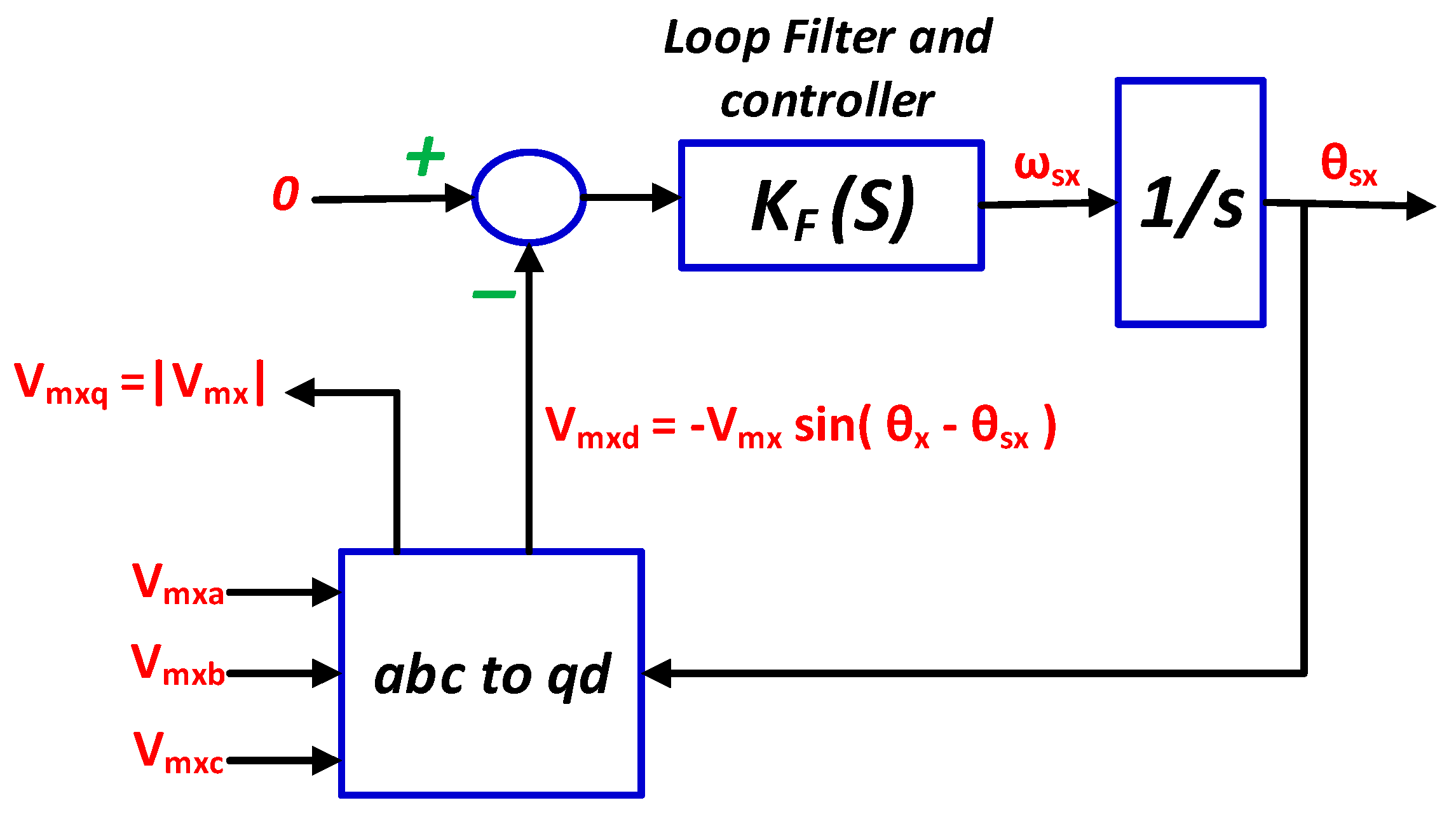
The phase-locked loop (PLL) is designed and applied to each DG unit to monitor the frequency of the system and define a reference frequency for the q d   transformation. The dynamic equations of the PLL are added to the system equations to make them more practical. The three-phase PLL, as illustrated in Figure 6, takes the measured local load voltage and transforms it into a q d -axis frame before comparing the   d -axis voltage to zero as a reference.
To eliminate noises, the error is sent via a controller and then a low-pass filter. The goal of the PLL is to align the voltage on the q -axis while keeping the voltage on the d -axis at zero, as a result:
V m x d   = V m x d sin ( θ x θ s x )  
If θ x θ s x is very small, we can presume:
V m x ( θ x θ s x ) K F s s = θ s x  
As a result, the closed-loop transfer function may be defined and compared to the denominator of the second-order conventional Butterworth filter transfer function as follows:
θ s x θ x = V m x K F s s + V m x K F s  
θ s x θ x = s V m x k P p l l + V m x k P p l l s 2 + s V m x k P p l l + V m x k I p l l = 2 ζ ω n 1 s + ω n 1 2 s 2 + 2 ζ ω n 1 s + ω n 1 2  
k P p l l = 2 ζ ω n 1 V m x   and   k I p l l = ω n 1 2 V m x  
where ω n 1 is the natural frequency, which is generally selected as 377 (rad/s), and ζ is the damping factor, which is usually chosen as the critical damping factor, which is 0.707.

2.2.5. Supervisory Control

Supervisory control is the process of overseeing and managing the operation of a microgrid, including monitoring both the generation and consumption stages, controlling the power flow, and ensuring the stability and reliability of the grid. There are several approaches to the supervisory control of a microgrid, including centralized and decentralized control [23]. In centralized control, a single control center is responsible for overseeing the operation of the microgrid. Centralized control systems are used in large-scale systems where it is important to have a single point of control and decision making. For example, a centralized control system might be used to control a power grid, industrial process, or transportation system. One advantage of centralized control systems is that they can be highly efficient and reliable, as the central controller can make decisions based on a comprehensive view of the entire system. Additionally, centralized control systems can be easier to design and implement, as all their control functions are centralized in a single location [28].
Centralized control is adopted in this study to regulate both the frequency and voltage in order to maintain a stable point of operation in the presence of the unpredictable and uncertain nature of loads. The developed supervisory control in this study monitors both the frequency and voltage and calculates the net change in the required power, according to the changes in the demand. In this study, a PI controller is compared to a regression tree algorithm for supervisory control, as shown in the diagram below. In Figure 7, the outputs form the supervisory control using either a PI controller or regression tree algorithm and are supplied to the droop control, as shown in Figure 3.

3. Regression Tree Algorithm

A regression tree is a type of decision tree that is used for regression tasks rather than classification tasks. In regression, the goal is to predict a continuous numerical value, rather than a discrete class label. A regression tree is a supervised learning algorithm, meaning that it requires a labeled training dataset to learn from [29]. The algorithm begins by identifying the feature that best splits the training data into distinct classes. It then splits the data into subsets based on the value of this feature and the process is repeated for each subset until the tree is fully grown. The resulting tree can then be used to make predictions on new, unseen data by traversing the tree and making decisions based on the values of the features in the data. A regression tree predicts the numerical value for a leaf node in the tree. This value is computed as the mean of the target values for the samples that fall into that leaf. Regression trees are useful because they can handle a mix of numerical and categorical features, and they can also handle non-linear relationships between the features and targets [30]. However, regression trees can be prone to overfitting, especially if the tree is allowed to grow too deep. To prevent this overfitting, regression trees can be pruned by removing unnecessary branches or setting limits on the depth of the tree.
To create a regression tree, the measure of the “goodness” of a split should be defined. One common measure is the mean squared error (MSE). Given a set of training examples and their corresponding target values, the MSE of a split is defined as the sum of the squared differences between the predicted value and true value, divided by the number of examples in the split [30].
The process of constructing a regression tree can be described as follows:
  • Start with the entire dataset and calculate the MSE (or another chosen criterion) for the current group.
  • Consider each possible split of the data based on the values of the predictor variables.
  • For each split, calculate the MSE (or other chosen criterion) for each of the resulting subgroups.
  • Choose the split that results in the lowest overall MSE (or another chosen criterion).
  • Repeat steps 2–4 for each of the resulting subgroups until the tree is fully constructed.
The mathematical expression for the MSE criterion is defined as (1):
M S E = 1 n * y y ˇ 2
where:
  • n is the number of observations in the data.
  • y is the actual value of the target variable for a given observation.
  • y ˇ is the predicted value of the target variable for a given observation.
This equation is used to calculate the MSE for each subgroup at each step in the tree construction process. The split that results in the lowest overall MSE is chosen as the next split in the tree.

3.1. Dataset

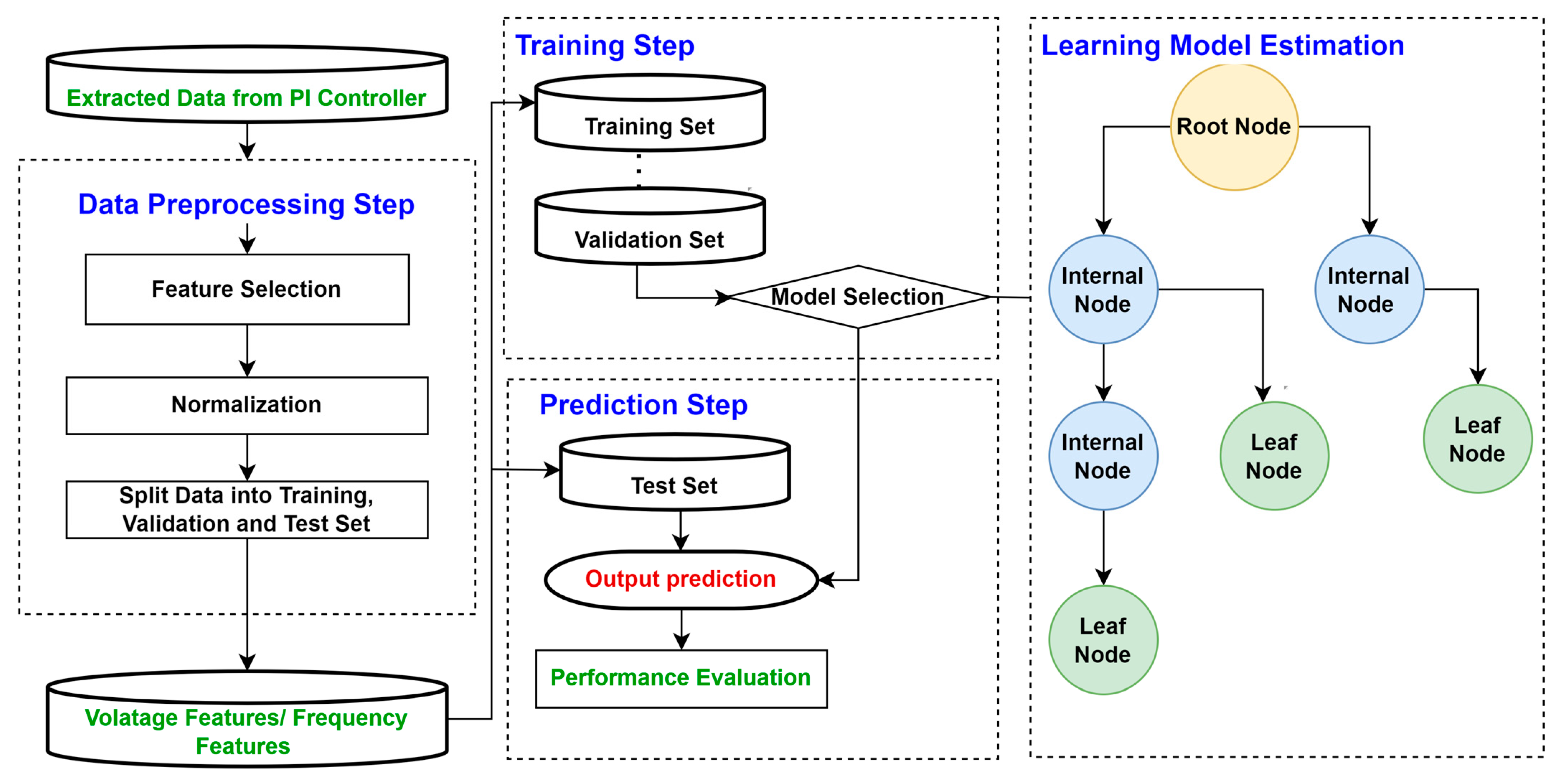
A supervised learning algorithm, such as the tree algorithm, requires training with relevant data. The training data for the tree algorithm in this study were obtained from the operation of the microgrid system using a PI controller for the supervisory control. The dataset comprised 1.2 million datasets, which were divided into training, testing, and validation. The validation test helped to determine the predictive accuracy of the model, and this helped to prevent overfitting. A k-fold cross-validation was utilized. K-fold cross-validation is a resampling procedure used to evaluate the performance of machine learning models. It splits the data into k disjoint folds. For each validation fold, it trains the model using the training fold data (the data not in the validation fold). Then, it assesses the model performance using the validation fold data and calculates the average validation error over all the folds [31]. This method is effective in predicting the accuracy of the final model trained with the entire dataset. A five-fold validation was adopted in this study.

3.2. Preprocessing

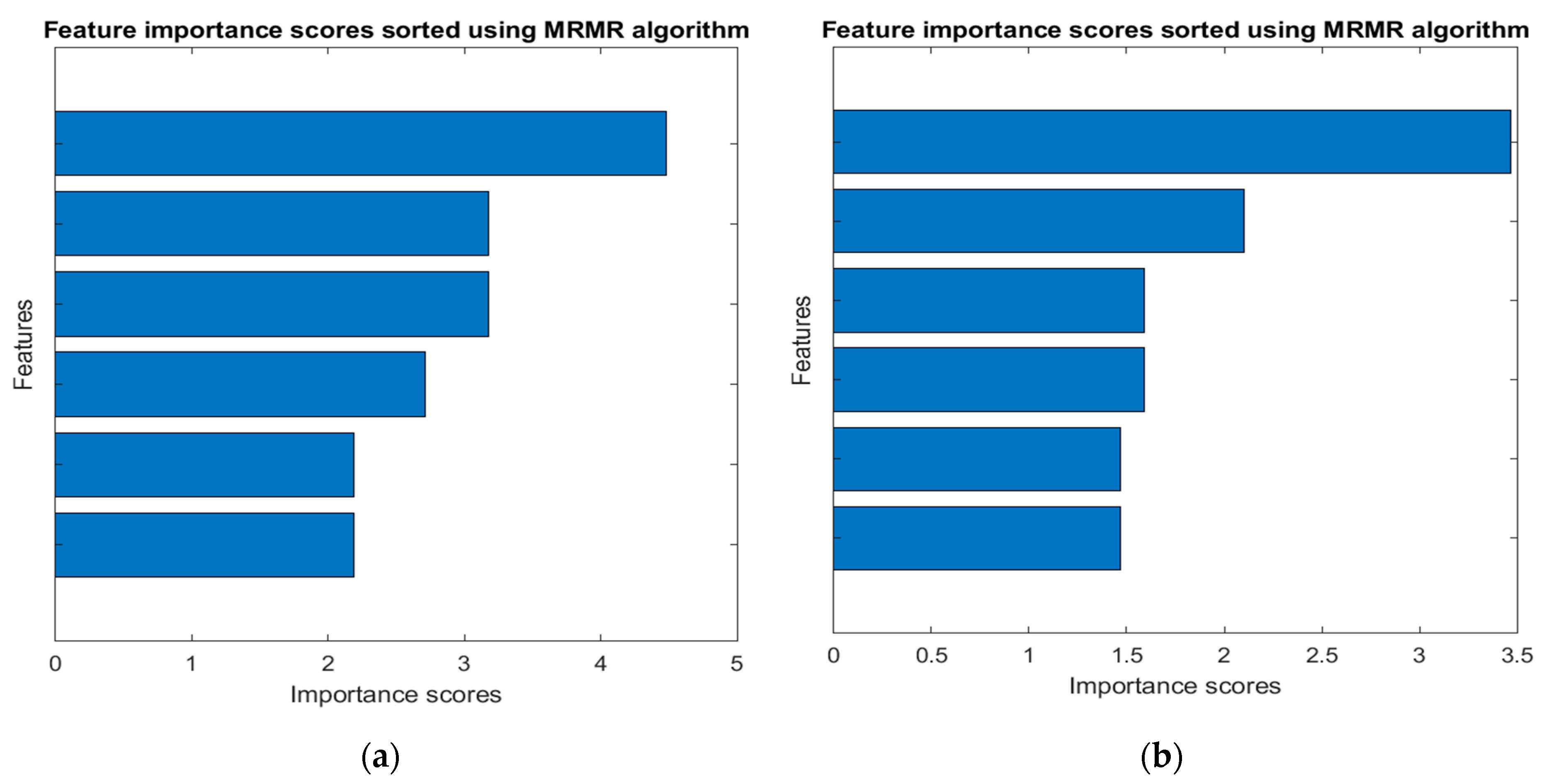
The input features for training the regression tree algorithm were reduced to four features using minimal redundancy maximal relevance (mRMR) [32]. An mRMR is a feature selection algorithm that aims to identify a subset of features that are highly relevant to the target variable and have a low redundancy with each other. The algorithm seeks to find an optimal set S of features that maximizes V s   2 , the relevance of S with respect to a response variable y , and minimizes W s   3 , the redundancy of     S . The maximization and minimization are represented with mutual information I [31,33].
V s = 1 S x   ϵ S I x , y
W s = 1 S 2 x , z   ϵ S I x , z
where S is the number of features S .
The four input features were rescaled into range of 0 and 1. Rescaling is a technique used to transform the values of a feature so that they have a specific range or distribution. This is often performed in machine learning to ensure that the features are within a comparable scale, which can help to improve the performance of certain algorithms. A min-max scaling in (4) was applied in this study to scale the features into a specific range of 0 and 1 [31].
S r e s c a l e d = a + S m i n s m a x s m i n s b a
where S, m a x s ,   and   m i n s are the number of selected features and the maximum and minimum values of the features, respectively. b and a are 1 and 0, respectively.
The flowchart of the system implementation is shown in Figure 8. Table 1 presents the simulation system parameters.

4. Simulation Results and Discussion

Figure 1, with the three converters as DG units, was simulated in the MATALB/Simulink software to test the system and controllers. The regression tree algorithm was trained using the dataset obtained from the optimal operation of the PI supervisory control. Initially, six features were extracted for each of the supervisory control units, which were eventually reduced to four using mRMR, with the highest importance scores as shown in Figure 9 and Table 2.
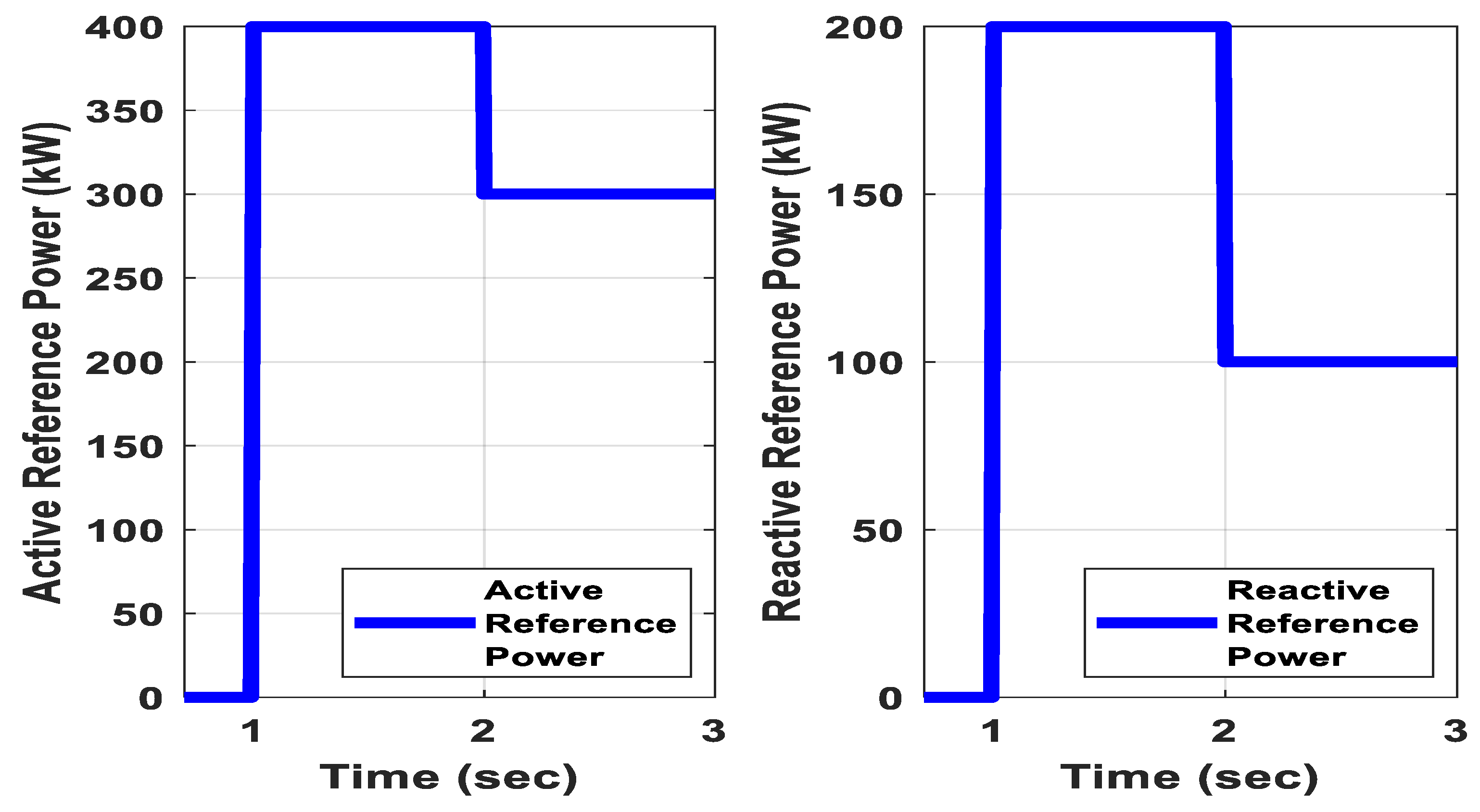
These features and targets comprised 1.2 million data points for both the frequency and voltage supervisory control units. These features were rescaled between 0 and 1 using Equation (4). The effectiveness of the regression tree algorithm and PI controller was evaluated in relation to the dynamic response when the load was subjected to step change in both its active and reactive power, as shown in Figure 10. The step change was introduced at 1 and 2 s. The dynamic system responses are shown in Figure 11, Figure 12 and Figure 13.
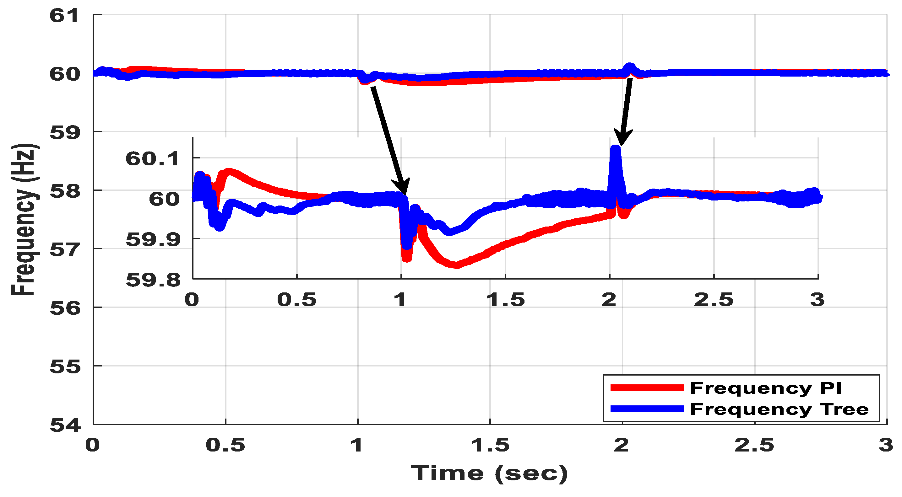
It is important to maintain a stable frequency in a power system, as deviations from the nominal frequency can cause problems with the operation of the equipment and lead to power outages. The supervisory control unit was designed to maintain a stable 60 Hz frequency operation. The droop active power/frequency was set to 1%. This implies that the microgrid frequency could vary its frequency between 60.3 Hz when the inverter produced no active power and 59.7 Hz when the inverter produced its nominal active power.
The rescaled features within the range of 0 and 1 were supplied to the regression tree algorithm, which made the prediction and generated the output response in relation to the input. Table 3 shows the step response analysis of the frequency. The results in Figure 11 and Figure 12 show the response of the frequency and active power at the PCC to the sudden change in the load demand. It is evident from Figure 11 and Figure 12 and Table 3 that tree algorithms attain the reference frequency within a minimal time with minimal overshoot and undershoot.
Voltage stability refers to the ability of a microgrid system to maintain a stable voltage at the load side, despite changes in the power demand or generation. If the voltage becomes unstable, it can lead to power quality issues, equipment damage, and blackouts. To ensure this voltage stability in a microgrid system, it is important to properly design and control the system’s power generation and distribution. The supervisory controller was designed to maintain a 600 V stable operation at the PCC. The ratio of the droop reactive power to the voltage was set to 4%. As a result, the PCC bus was allowed to fluctuate from 612 Vrms, the inverter’s full inductive power, to 588 Vrms, the inverter‘s full capacitive power. The rescaled features between 0 and 1 were supplied to the regression to generate the appropriate voltage, in order to maintain a stable point of operation at the PCC. The results in Figure 12 and Figure 13 show the response of the voltage and reactive power at the PCC, respectively, to the sudden change in the load demand. Using the “stepinfo” command in MATLAB, Table 4 shows the response analysis of the voltage. It is evident from Figure 12 and Figure 13 and Table 4 that tree algorithms attain the reference voltage with less overshoot and settling minimums.
Harmonic distortion refers to the presence of harmonic frequencies in an electrical current or voltage that are not present in the original waveform. Harmonics are multiples of the fundamental frequency of the waveform, and they can be either odd- or even-ordered. Harmonics can be caused by a variety of sources, such as nonlinear loads, power electronic devices, and electrical equipment that is not designed to operate at a particular frequency.
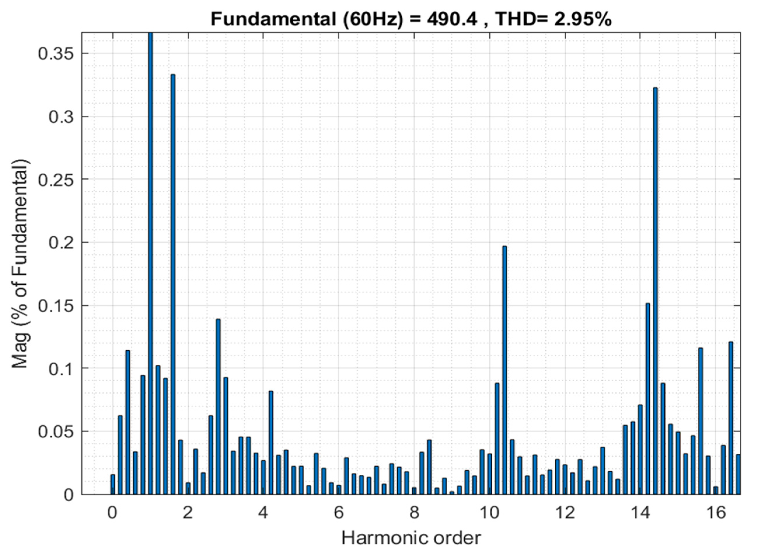
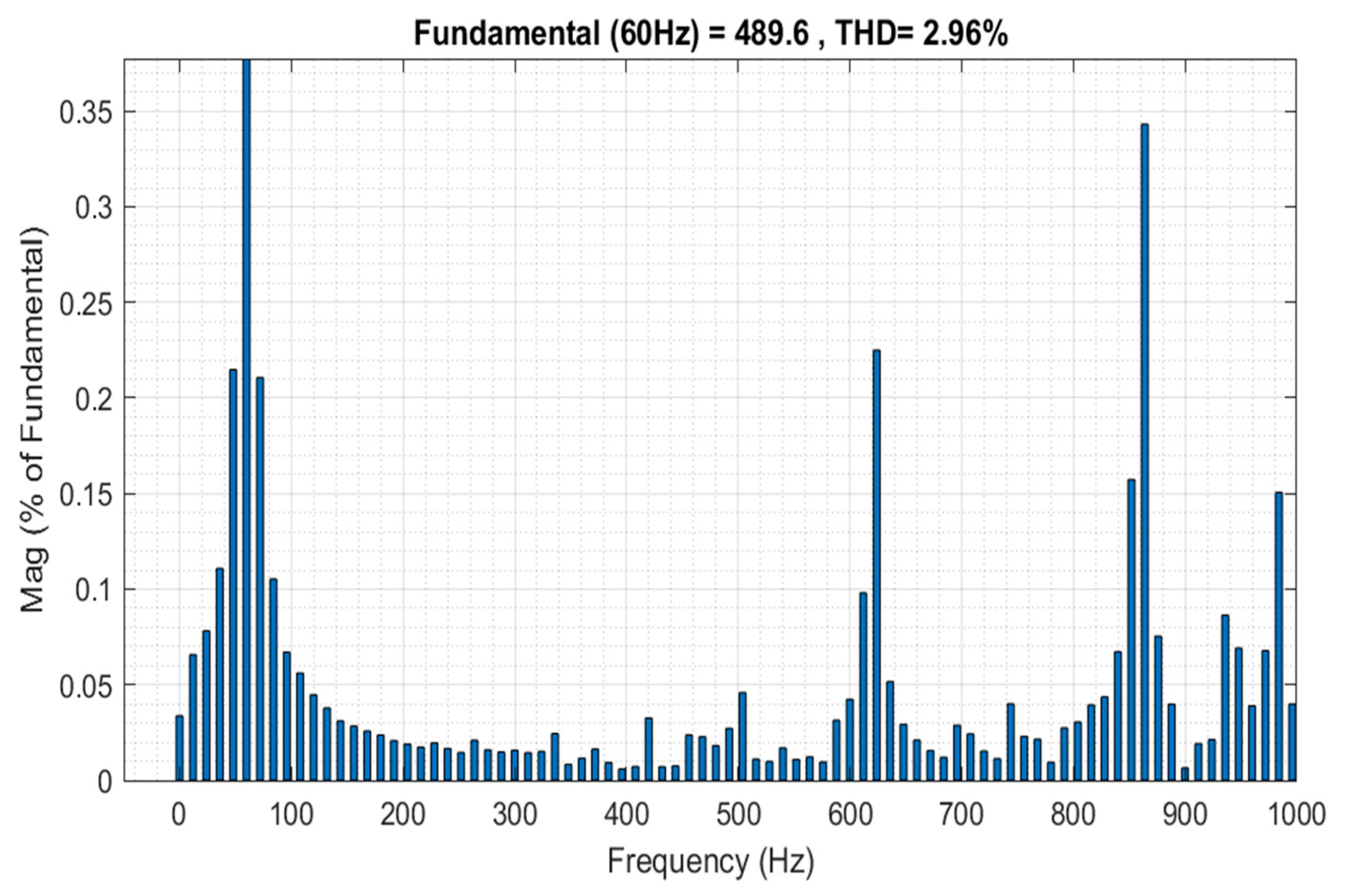
To generate the characteristics of the harmonics, fast Fourier transform (FFT) in the MATLAB Simulink method was used for the analysis. It is clearly shown in Figure 14 and Figure 15 that the voltage distortion with the PI and regression tree algorithms at the PCC was less than the permissible value of 5%, according to the IEEE 519 power harmonic standards. Generally, the influence of the harmonic voltage distortion on the power grid can be ignored.

5. Conclusions

In this study, we presented a novel droop control strategy for load sharing among three autonomous converter power systems, using a machine learning approach. Our proposed method relied on a regression tree algorithm to regulate both the system frequency and terminal voltage at the PCC. The simulation results clearly demonstrate the effectiveness of this approach, as evidenced by the improved step response and harmonic distortion in the system. Specifically, our results showed that the regression tree algorithm outperformed the traditional PI controller in terms of its response speed and accuracy, while also maintaining a lower level of harmonic distortion. Our findings have significant implications for the design and operation of microgrid systems, as they suggest that machine learning techniques may be a promising approach for improving the stability and efficiency of these systems. By using machine learning, we were able to develop a control strategy that was more responsive, more accurate, and less prone to harmonic distortion than the traditional methods. The benefits of our approach were observed in both the step response and harmonic distortion, which are critical factors in the stability and efficiency of microgrid systems. In conclusion, our study has demonstrated the effectiveness of using a regression tree algorithm for the supervisory control of droop-based grid-forming inverters in islanded mode. The results suggest that machine learning techniques may be a promising approach for improving the stability and efficiency of microgrid systems, and further research is needed to confirm these findings and explore the potential of machine learning techniques in other areas of microgrid control.

Author Contributions

Conceptualization, A.A.A.-S. and H.M.H.F.; methodology, M.A.; software, H.O.O.; validation, A.A.A.-S., H.M.H.F. and F.A.; formal analysis, A.A.; investigation, U.B.; resources, K.E.A.; data curation, A.M.A.; writing—original draft preparation, H.O.O.; writing—review and editing, A.A.A.-S.; visualization, A.M.A.; supervision, A.A.A.-S. and K.E.A.; project administration, M.A.; funding acquisition, M.A. All authors have read and agreed to the published version of the manuscript.

Funding

This research received no external funding.

Institutional Review Board Statement

Not applicable.

Informed Consent Statement

Not applicable.

Data Availability Statement

No new data were created or analyzed in this study.

Acknowledgments

The authors extend their appreciation to the Deputyship for Research & Innovation, “Ministry of Education” in Saudi Arabia for funding this research work through the project number (IFKSUDR_E141).

Conflicts of Interest

The authors declare no conflict of interest.

References

  1. Dong, J.; Gong, C.; Chen, H.; Wang, Z. Secondary frequency regulation and stabilization method of islanded droop inverters based on integral leading compensator. Energy Rep. 2022, 8, 1718–1730. [Google Scholar] [CrossRef]
  2. Feng, C.-Y.; Yang, X.; Afshan, S.; Irfan, M. Can renewable energy technology innovation promote mineral resources’ green utilization efficiency? Novel insights from regional development inequality. Resour. Policy 2023, 82, 103449. [Google Scholar] [CrossRef]
  3. Borhanazad, H.; Mekhilef, S.; Gounder Ganapathy, V.; Modiri-Delshad, M.; Mirtaheri, A. Optimization of micro-grid system using MOPSO. Renew. Energy 2014, 71, 295–306. [Google Scholar] [CrossRef]
  4. Alturki, F.A.; Omotoso, H.O.; Al-Shamma’a, A.A.; Farh, H.M.H.; Alsharabi, K. Novel Manta Rays Foraging Optimization Algorithm Based Optimal Control for Grid-Connected PV Energy System. IEEE Access 2020, 8, 187276–187290. [Google Scholar] [CrossRef]
  5. Al-Shamma’a, A.A.; Omotoso, H.O.; Noman, A.M.; Alkuhayli, A.A. Grey Wolf Optimizer Based Optimal Control for Grid-Connected PV System. In Proceedings of the IECON 2020 the 46th Annual Conference of the IEEE Industrial Electronics Society, Singapore, 20–21 October 2020; pp. 2863–2867. [Google Scholar] [CrossRef]
  6. Mohammed, N.; Ciobotaru, M. Adaptive Power Control Strategy for Smart Droop-based Grid-connected Inverters. IEEE Trans. Smart Grid 2022, 13, 2075–2085. [Google Scholar] [CrossRef]
  7. Safiullah, S.; Rahman, A.; Lone, S.A.; Hussain, S.M.S.; Ustun, T.S. Robust frequency–voltage stabilization scheme for multi-area power systems incorporated with EVs and renewable generations using AI based modified disturbance rejection controller. Energy Rep. 2022, 8, 12186–12202. [Google Scholar] [CrossRef]
  8. Cheng, C.; Xie, S.; Tu, L.; Tan, L.; Qian, Q.; Xu, J. Single Grid-Current Sensor-Controlled Weak-Grid-Following Inverters: A State-and-Disturbance-Observer-Based Robust Control Scheme Achieving Grid-Synchronization and Disturbance Rejection. IEEE Trans. Power Electron. 2022, 37, 13743–13754. [Google Scholar] [CrossRef]
  9. Kikusato, H.; Orihara, D.; Hashimoto, J.; Takamatsu, T.; Oozeki, T.; Matsuura, T.; Miyazaki, S.; Hamada, H.; Miyazaki, T. Performance evaluation of grid-following and grid-forming inverters on frequency stability in low-inertia power systems by power hardware-in-the-loop testing. Energy Rep. 2023, 9, 381–392. [Google Scholar] [CrossRef]
  10. Seguin, R.; Woyak, J.; Costyk, D.; Hambrick, J.C.; Mather, B.A. High-Penetration PV Integration Handbook for Distribution Engineers; National Renewable Energy Lab (NREL): Golden, CO, USA, 2016. [Google Scholar]
  11. Liserre, M.; Teodorescu, R.; Blaabjerg, F. Stability of photovoltaic and wind turbine grid-connected inverters for a large set of grid impedance values. IEEE Trans. Power Electron. 2006, 21, 263–272. [Google Scholar] [CrossRef]
  12. Hart, P.J.; Gong, M.; Liu, H.; Chen, Z.; Zhang, Y.; Wang, Y. Provably-Stable Overload Ride-Through Control for Grid-Forming Inverters Using System-Wide Lyapunov Function Analysis. IEEE Trans. Energy Convers. 2022, 37, 2761–2776. [Google Scholar] [CrossRef]
  13. Song, Y.; Wang, X.; Blaabjerg, F. Impedance-Based High-Frequency Resonance Analysis of DFIG System in Weak Grids. IEEE Trans. Power Electron. 2017, 32, 3536–3548. [Google Scholar] [CrossRef]
  14. Sun, Y.; Li, L.; Shi, G.; Hou, X.; Su, M. Power Factor Angle Droop Control—A General Decentralized Control of Cascaded Inverters. IEEE Trans. Power Deliv. 2021, 36, 465–468. [Google Scholar] [CrossRef]
  15. Mohammed, N.; Kerekes, T.; Ciobotaru, M. Communication-Free Equivalent Grid Impedance Estimation Technique for Multi-Inverter Systems. IEEE Trans. Ind. Electron. 2023, 70, 1542–1552. [Google Scholar] [CrossRef]
  16. Kroposki, B.; Johnson, B.; Zhang, Y.; Gevorgian, V.; Denholm, P.; Hodge, B.; Hannegan, B. Achieving a 100% Renewable Grid: Operating Electric Power Systems with Extremely High Levels of Variable Renewable Energy. IEEE Power Energy Mag. 2017, 15, 61–73. [Google Scholar] [CrossRef]
  17. Mohammed, N.; Lashab, A.; Ciobotaru, M.; Guerrero, J.M. Accurate Reactive Power Sharing Strategy for Droop-Based Islanded AC Microgrids. IEEE Trans. Ind. Electron. 2023, 70, 2696–2707. [Google Scholar] [CrossRef]
  18. Hu, Q.; Han, R.; Quan, X.; Wu, Z.; Tang, C.; Li, W.; Wang, W. Grid-Forming Inverter Enabled Virtual Power Plants with Inertia Support Capability. IEEE Trans. Smart Grid 2022, 13, 4134–4143. [Google Scholar] [CrossRef]
  19. Unruh, P.; Nuschke, M.; Strauß, P.; Welck, F. Overview on Grid-Forming Inverter Control Methods. Energies 2020, 13, 2589. [Google Scholar] [CrossRef]
  20. Ko, H.-S.; Jang, M.-S.; Ryu, K.-S.; Kim, D.-J.; Kim, B.-K. Supervisory Power Quality Control Scheme for a Grid-Off Microgrid. IEEE Trans. Sustain. Energy 2018, 9, 1003–1010. [Google Scholar] [CrossRef]
  21. Lundberg, M.; Samuelsson, O.; Hillberg, E. Local voltage control in distribution networks using PI control of active and reactive power. Electr. Power Syst. Res. 2022, 212, 108475. [Google Scholar] [CrossRef]
  22. Sharma, D.; Sadeque, F.; Mirafzal, B. Synchronization of Inverters in Grid Forming Mode. IEEE Access 2022, 10, 41341–41351. [Google Scholar] [CrossRef]
  23. Al Badwawi, R.; Issa, W.R.; Mallick, T.K.; Abusara, M. Supervisory Control for Power Management of an Islanded AC Microgrid Using a Frequency Signalling-Based Fuzzy Logic Controller. IEEE Trans. Sustain. Energy 2019, 10, 94–104. [Google Scholar] [CrossRef]
  24. Tursini, M.; Parasiliti, F.; Zhang, D. Real-time gain tuning of PI controllers for high-performance PMSM drives. IEEE Trans. Ind. Appl. 2002, 38, 1018–1026. [Google Scholar] [CrossRef]
  25. Kalaam, R.; Muyeen, S.M.; Al-Durra, A.; Hasanien, H.; Al-Wahedi, K. Optimization of Controller Parameters for Grid-tied Photovoltaic System at Faulty Network using Artificial Neural Network based Cuckoo Search Algorithm. IET Renew. Power Gener. 2017, 11, 1517–1526. [Google Scholar] [CrossRef]
  26. Sanchis, R.; Peñarrocha-Alós, I. A new method for experimental tuning of PI controllers based on the step response. ISA Trans. 2022, 128, 329–342. [Google Scholar] [CrossRef] [PubMed]
  27. Ghalebani, P.; Niasati, M. A distributed control strategy based on droop control and low-bandwidth communication in DC microgrids with increased accuracy of load sharing. Sustain. Cities Soc. 2018, 40, 155–164. [Google Scholar] [CrossRef]
  28. Chen, G.; Li, Z.; Zhang, Z.; Li, S. An Improved ACO Algorithm Optimized Fuzzy PID Controller for Load Frequency Control in Multi Area Interconnected Power Systems. IEEE Access 2020, 8, 6429–6447. [Google Scholar] [CrossRef]
  29. Eslami, A.; Negnevitsky, M.; Franklin, E.; Lyden, S. Review of AI applications in harmonic analysis in power systems. Renew. Sustain. Energy Rev. 2022, 154, 111897. [Google Scholar] [CrossRef]
  30. Shalizi, C.R. Advanced Data Analysis from an Elementary Point of View; Cambridge University Press: Cambridge, UK, 2012. [Google Scholar]
  31. The Mathworks. Statistics and Machine Learning Toolbox. Available online: https://www.mathworks.com/help/releases/R2022a/pdf_doc/stats/stats.pdf (accessed on 1 March 2023).
  32. Chen, C.; Yan, X. Optimization of a Multilayer Neural Network by Using Minimal Redundancy Maximal Relevance-Partial Mutual Information Clustering With Least Square Regression. IEEE Trans. Neural Netw. Learn. Syst. 2015, 26, 1177–1187. [Google Scholar] [CrossRef]
  33. Ding, C.; Peng, H. Minimum redundancy feature selection from microarray gene expression data. J. Bioinform. Comput. Biol. 2005, 3, 185–205. [Google Scholar] [CrossRef]
Figure 1. Schematic diagram of the microgrid.
Sustainability 15 08018 g001
Figure 2. System control unit.
Sustainability 15 08018 g002
Figure 3. Droop control unit.
Sustainability 15 08018 g003
Figure 4. Schematic diagram of voltage control.
Sustainability 15 08018 g004
Figure 5. Schematic inner current control units.
Sustainability 15 08018 g005
Figure 6. Block diagram of PLL.
Sustainability 15 08018 g006
Figure 7. (a) Voltage; and (b) frequency supervisory control.
Sustainability 15 08018 g007
Figure 8. Framework of the proposed model.
Sustainability 15 08018 g008
Figure 9. (a) Frequency; and (b) voltage feature reductions.
Sustainability 15 08018 g009
Figure 10. Load reactive and active power reference.
Sustainability 15 08018 g010
Figure 11. Frequency at PCC.
Sustainability 15 08018 g011
Figure 12. Active power measured at PCC.
Sustainability 15 08018 g012
Figure 13. Reactive power at PCC.
Sustainability 15 08018 g013
Figure 14. Regression tree FFT analysis of voltage distortion at PCC.
Sustainability 15 08018 g014
Figure 15. PI FFT analysis of voltage distortion at PCC.
Sustainability 15 08018 g015
Table 1. The parameters of the DG unit.
ParametersValues
V m x 600 V
F n v 60 Hz
P400 kW
Q100 kW
F s w 2.7 kHz
Mpx1%
Nqx4%
V d c x 1000 V
P 1 , P 2 , P 3 500, 300, 200 kW
Table 2. Features of the supervisory control.
Frequency FeaturesVoltage Features
Measured active power at PCCMeasured reactive power at PCC
Measured frequency at PCCProportional parameter of PI controller
Derivative of PI controllerDerivative of PI controller
Integral of PI controllerIntegral of PI controller
Table 3. Step response analysis.
ResponsePITree
Settling minimum (V)59.833259.8808
Settling maximum (V)60.066460.0586
Overshoot (pu)0.11060.0976
Peak (V)60.066460.0586
Peak time (s)0.17010.0342
Table 4. Voltage step response analysis.
ResponsePITree
Settling minimum (V)479.9482
Settling maximum (V)611.2616606.623
Overshoot (pu)1.87691.1038
Peak (V)611.2616606.623
Peak Time (s)0.23140.9918
Disclaimer/Publisher’s Note: The statements, opinions and data contained in all publications are solely those of the individual author(s) and contributor(s) and not of MDPI and/or the editor(s). MDPI and/or the editor(s) disclaim responsibility for any injury to people or property resulting from any ideas, methods, instructions or products referred to in the content.