Article

An Analysis of Dynamics of Retaining Wall Supported Embankments: Towards More Sustainable Railway Designs

1
School of Civil Engineering, Southwest Jiaotong University, Chengdu 610031, China
2
MOE Key Laboratory of High-Speed Railway Engineering, School of Civil Engineering, Southwest Jiaotong University, Chengdu 610031, China
3
School of Civil Engineering, University of Leeds, Leeds LS2 9JT, UK
*
Author to whom correspondence should be addressed.
Sustainability 2023, 15(10), 7984; https://doi.org/10.3390/su15107984
Submission received: 3 April 2023 / Revised: 7 May 2023 / Accepted: 10 May 2023 / Published: 13 May 2023
(This article belongs to the Special Issue Sustainability and Innovation in Transport Infrastructure Geotechnics)

Abstract

:
Retaining walls are structures used to retain earth materials on a slope. Typically, they are designed for static loads, but for highway and railway infrastructures, vehicle-induced dynamic responses are also relevant. Therefore, retaining wall structures are often designed with a factor of safety that is higher than necessary, because it can be challenging to quantify the magnitude of expected dynamic stresses during the design stage. This unnecessary increase in material usage reduces the sustainability of the infrastructures. To improve railway retaining wall sustainability, this paper presents the results from a field monitoring campaign on a heavy-haul rail line with a retaining wall, studying the dynamics induced in response to 30-ton axle load trains running at speeds of between 5 km/h and 100 km/h. The site comprises an earth embankment supported by a gravity retaining wall, with accelerometers on the sleepers, roadbed surface, and retaining wall, velocity sensors on the roadbed, and strain gauges on the rail web to record wheel–rail forces. The vibration intensities collected from various locations are processed to explore the peak particle velocities, maximum transient vibration values, and one-third octave band spectrums. Two transfer functions define the vibration transmission characteristics and attenuation of vibration amplitude along the propagation path. The long-term dynamic stability of the track formation is studied using dynamic shear strain derived from the effective velocity. The peaks of observed contact forces and vibrations are statistically analyzed to assess the impact of train speed on the dynamic behavior of the infrastructure system. Next, a 3D numerical model expresses the maximum stress and displacements on the roadbed surface as a function of train speed. The model evaluates the earth pressures at rest and vehicle-induced additional earth pressures and horizontal wall movement. The investigation provides new insights into the behavior of railway track retaining walls under train loading, and the field data are freely available for other researchers to download. The findings could facilitate the design of more sustainable retaining walls in the future.

1. Introduction

Heavy-haul traffic volumes are growing in many countries around the world [1]. These high axle loads can induce elevated strains in the track substructure, causing non-linear soil stiffness and damping [2,3,4]. This results in premature degradation and increased maintenance costs [5,6]. This is in-part due to the dynamic impact of heavier trains [7] with poor suspension on rail infrastructure [8,9]. In addition, a limited understanding of vehicle-induced dynamic responses often results in conservative infrastructure designs (with higher construction costs than necessary) [10]. This is due to the difficulty in accurately quantifying expected dynamic stresses during the design stage [11,12]. Unfortunately, this leads to unnecessary material usage and reduces infrastructure sustainability. Therefore, further clarification of the dynamic interaction between heavy-haul trains and earth substructures is crucial.
Ground- and structure-borne vibrations result from moving trains and the dynamic interaction between wheels, rails, track components, and foundations [13,14]. Vibrations induced by heavy-haul trains can be influenced by several factors, such as vehicle configurations, wheel–rail contact conditions, track geometry, and the dynamic properties of the support [15,16,17]. Through the sleepers, the pressure extends into the track foundation. The train configuration, speed, and sleeper spacing affect vibration generation and propagation through the ground [18,19]. Vibrational modes of the rail track are also controlled by the resonant frequencies of the track infrastructure elements [20,21], including both in-phase and out-of-phase vibrations, depending on the train speed. Vibrations from moving trains are transmitted through the railway track superstructure to the foundation, which comprises mainly nonhomogeneous materials (ballast and soil). Such media exhibit different properties between layers that determine the features of elastic wave propagation [22,23,24]. The vibro-impacts received from the rolling stock result in track structure deformation and subgrade stress. Hence, the magnitude and the distribution pattern of stresses over an area will be affected by axle load and spacing, types of track components, and the subgrade itself [25,26,27].
Railways built in mountainous regions often require the use of retaining walls [28]. When a retaining wall is introduced as part of the track infrastructure to retain the embankment fill, its dynamic response to train passage should also be considered [29], particularly for heavy-haul rail lines. However, long-term railway operations may be adversely affected by the additional deformation on the roadbed caused by retaining structures [30]. This is where the Geosynthetically Reinforced Soil with Retaining Wall (GRS-RW) system can be applied [31,32]. In China, stability issues associated with railway retaining structures must be examined using the Code for Design of Retaining Structures of Railway Earthworks (TB 10025-2019) [33]. The dynamic behavior of railway retaining walls and their interactions within the infrastructure system during train passage are not well-documented. These retaining wall structures are often designed with a factor of safety that is higher than necessary due to limited knowledge of their serviceability and field performance. As a result, there is an unnecessary increase in material usage, which reduces the sustainability of the structure.
This study aims to enhance the understanding of rail infrastructure serviceability for more sustainable railway designs. Firstly, a rail embankment with gravity retaining walls on a heavy-haul railway was monitored, followed by a numerical investigation of the railway system. The vibration responses of the sleeper, roadbed surface, retaining wall, and wheel–rail contact force were recorded for 30 passages of heavy-haul trains at various operating speeds. The track irregularities were documented as a reference before testing. The study focuses on the dynamic behavior of the railway system through in situ geotechnical instrumentation, analysis of wheel–rail forces and their propagation through the track elements, and the quasi-static behavior of the railway retaining wall. The field and numerical data presented aim to be useful for future modelling of heavy-haul railway systems, particularly those with retaining structures.

2. Field Monitoring

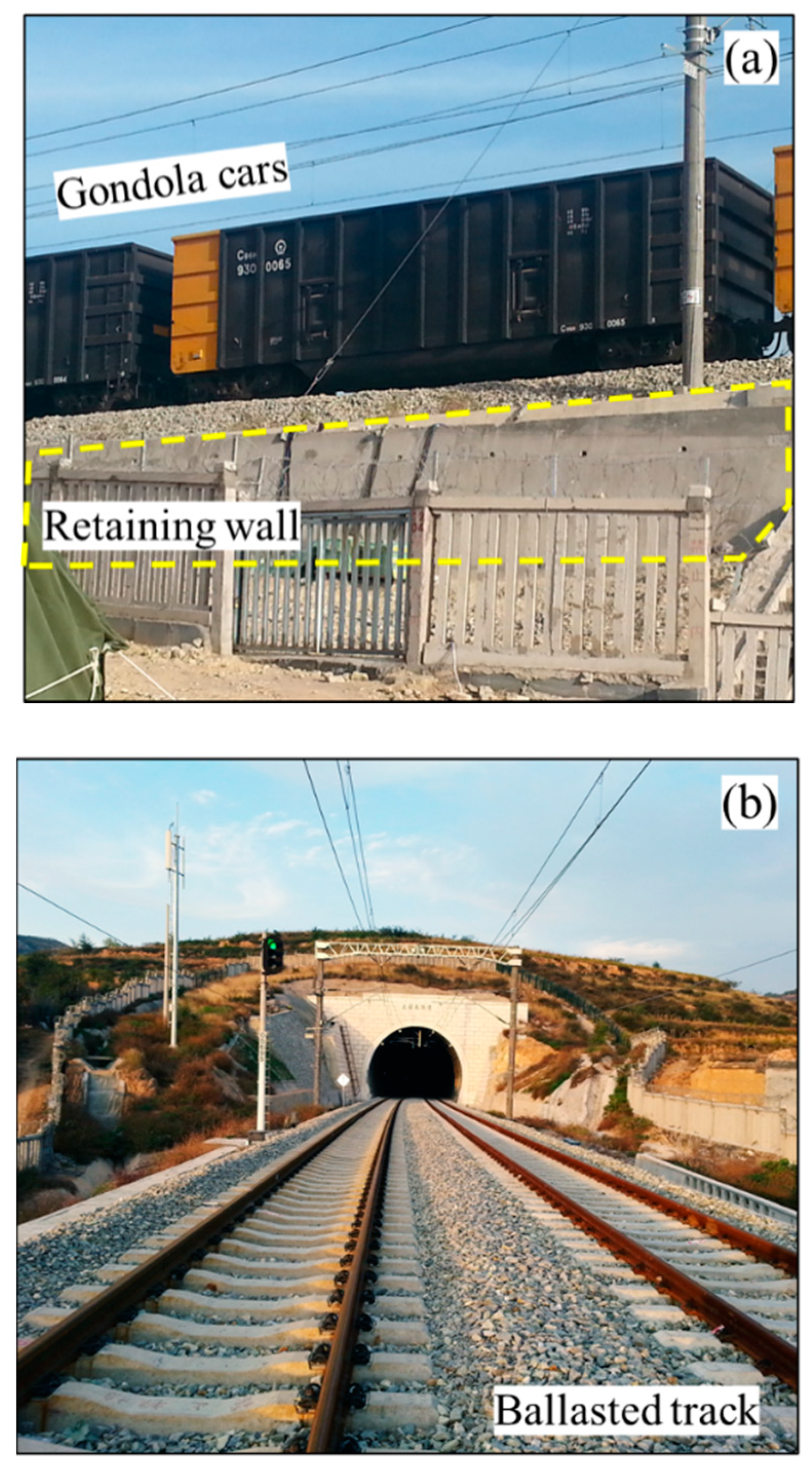
2.1. Site Description

The Watang–Rizhao railway, also referred to as the Jinyulu railway, is an electrified, double-track, heavy-haul rail that crosses northern China; it is 1260 km in length. As the first heavy freight railway line in China, with a maximum axle load of 30 tons, it is designed to transport 200 million tons of freight annually; the maximum line speed is 120 km/h. As illustrated in Figure 1, the test site is in southeast Shanxi, close to the border with Henan Province, mileage DK 551+870.25.
A cross-section of the instrumented earthworks is depicted in Figure 2. The ballasted track is constructed with prestressed concrete sleepers and a 60 kg/m rail. The ballast layer has a thickness of 0.35 m; it is supported by a 0.6-m-thick graded gravel roadbed, underlain by 1.9-m-thick Class-A fill at 95% compaction level (roadbed) and 2.7-m-thick Class-A fill at 92% compaction level (subgrade). Note that the fill is classified according to the Code for Design of Railway Earth Structure (TB 10001-2016) [34] and that Class A fill generally consists of well-graded gravelly soil with less than 15% fines. The formation slopes are at 4% for drainage, and the gradient of the embankment slope is 1:1.5. A gravity retaining wall made of C25 concrete (the characteristic strength of the concrete after 28 days of curing increases to 25 MPa) is constructed to the left of the route to provide lateral confinement. The retaining wall is 5 m high, 17.38 m long, and 1.05 m wide, at an inclined angle of 1:0.25. Its foundation is backfilled with compacted earth to enhance its strength. It was planned to run the test train (Figure 3a) on the left track, close to the retaining wall. A general view of the ballasted track structure is provided in Figure 3b.
The test section is downhill at a gradient of 10‰ toward the port of Rizhao. The elevation of the left rail is higher than that of the right rail, giving a 20 mm superelevation. To examine the track geometry quality prior to testing, a DS3 digital level was used to measure track irregularities. This device is suitable for third and fourth order levelling in China and has a measuring accuracy of ±1.5 mm. Note that Grade DS3 means the standard deviation for 1-km-long double-run levelling does not exceed 3 mm and the differential levelling misclosure (unit: mm) for the third and fourth order levelling does not exceed 12 L and 20 L respectively, where L is the distance (km) of a circuit or between bench marks. The test range includes 105 sleepers numbered in sequence from #0 to #104. Sleeper spacing is 0.6 m, yielding a total length of 0.6 × 104 = 62.40 m for the longitudinal range. Fourteen test points were set up at a spacing of 4.8 m. Table 1 shows the elevation readings for the left and right rails and the cross-level results. As required in the Code for Design of Railway Track (TB 10082-2017) [35], the ballasted track on the mainline of heavy-haul railways with an operating speed of less than 120 km/h shows that the allowable elevation difference in both rails is 4 mm. The maximum value of the measured data is 4 mm, satisfying the management requirements of static track irregularities.
The chord measuring method was used to measure the longitudinal level, as is illustrated in Figure 4, and the track geometry was derived from the offset measured at an intermediate point of a straight-line chord. Based on the measured data presented in Table 1, the longitudinal levels were plotted against chord lengths of 9.6, 19.2, 28.8, 38.4, 48.0, and 57.6 m in Figure 4, where a positive value indicates that the rail bulges upward. Under the same chord length conditions, the longitudinal levels vary at different locations, accompanied by direction changes. The variations are significant for chord lengths of 28.8 m and 38.4 m. However, the difference in the cross level of similar locations is much less significant, reflecting that the cross level is within tolerances. The section at a distance of 38.4 m to 52.8 m from the #0 sleeper (namely, from sleepers #64 to #88) has been identified to have poor track geometry; the track irregularities there exceed 10 mm and 7 mm for the left and right rails, respectively, i.e., much higher than those of the other sections. Chord length significantly influences the longitudinal level—the maximum value of longitudinal levels for both rails is 4 mm at a 9.6 m chord length, but this value increases to 14–17 mm at chord lengths of 28.8 m and 38.4 m. According to the Code for Design of Railway Track (TB 10082-2017) [35], for the ballasted track on the mainline of heavy-haul railways with an operating speed of less than 120 km/h, the measured longitudinal level should be kept below 4 mm when a chord length of 10 m is used. The longitudinal level therefore meets the requirements for static track irregularities.

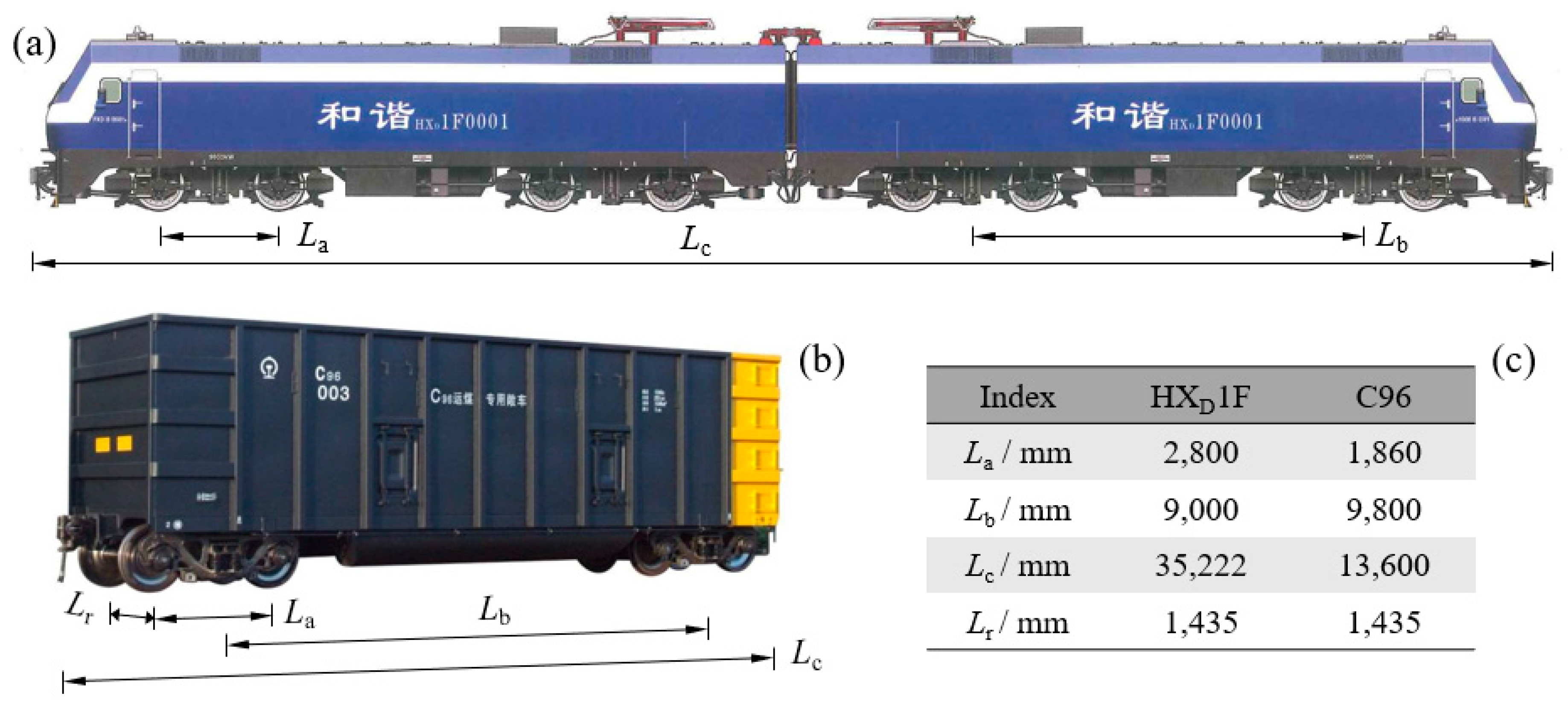
2.2. Instruments and Test Train

During the field monitoring, geotechnical instrumentation was utilized after removing the ballast (Figure 5a), which involved integrated vibration sensors, strain gauges, a data acquisition unit, and a signal amplifier. The physical dimensions of the integrated vibration sensors (Type 891-II, Figure 5b) are 56 mm × 56 mm × 77 mm [13]. Although the unidirectional vibration measurement system incorporates three main functions, i.e., displacement, velocity, and acceleration, only acceleration (at all positions) and velocity (on the roadbed surface) analyses are performed in this paper. The vibration sensors have a capacity, accuracy, and resolution of 2 × 104 mm/s2, 0.01 mm/s2, and 2 × 10⁻³ mm/s2, respectively. The gravity retaining wall, roadbed, and sleeper were instrumented with four vertical vibration sensors, as shown in Figure 2. Two sensors embedded at the formation level for acceleration and velocity testing were immediately beneath the one placed on the sleeper. Protective shields made of aluminum alloy housed the sensors to avoid potential damage from the ballast (Figure 5b). Meanwhile, fine sand was filled as a medium between the shield and the sensor. In contrast, the other two sensors for acceleration testing were adhered using glue. The ballast was backfilled and compacted after instrument installation.
The data acquisition system (Figure 5c) comprised a laptop, a data acquisition unit, and a signal amplifier. The signal amplifier was an accessory device used along with vibration sensors to provide essential data processing functions, including integration, filtering, and signal amplification. Upon receiving a weak signal, the signal amplifier was triggered to maximize the accuracy of the collected data. The data acquisition unit, manufactured by imc Test and Measurement GmbH (Berlin, Germany), can record data at up to 100 kHz per channel and was fully compatible with various instruments and signal amplifiers. In addition, after grinding (Figure 5d), strain gauges were glued to the rail web (Figure 5e) to measure the vertical wheel–rail force. Field calibration was conducted to reproduce actual work conditions (Figure 5f).
The test train configuration consisted mainly of two heavy-duty electric locomotives (type HXD1F) on both ends and forty-two C96-type gondola freight cars in the middle. Figure 6 shows the geometric characteristics of the locomotive and freight car; both are run with a rail gauge of 1435 mm. China’s leading type of B0-B0 AC drive electric locomotive is the HXD1F electric locomotive, which has an axle weight of 30 metric tons. The locomotive weighs 240 t and has a maximum speed of 100 km/h. The key dimensions, i.e., the axle spacing within a bogie La, bogie spacing Lb and vehicle length Lc, are 2800 mm, 9000 mm, and 35,222 mm respectively. Explicitly designed for coal transport, the C96-type freight car has an axle load of 30 t. The dimension indexes La, Lb, and Lc for C96 are 1860 mm, 9800 mm, and 13,600 mm, respectively. Tests were used to record 30 passages in total, with the train travelling at 5 km/h once for quasi-static calibrations. The monitoring in the field was then conducted at five speeds: 60, 70, 80, 90, and 100 km/h. Signals received by the instruments were used to calculate the actual speeds.

3. Analyses of Measured Data

3.1. Vibration Acceleration

Three acceleration records are compared at 100 km/h on the left side of Figure 7, where the acceleration signals are displayed for the passage of five C96 freight cars (full signals share a similar pattern). Black and red curves depict raw signals and running root-mean-square curves, respectively. The root-mean-square (RMS) amplitude format is valuable, because it indicates an oscillating signal’s equivalent steady-state energy value. The two most common settings used for the short-time average display of the signal waveform (moving window), i.e., fast and slow, have time constants of 0.125 s and 1.0 s, respectively. The RMS values in Figure 7 were derived by averaging the raw data point-by-point over a time constant of 1 s (slow window), as recommended by ISO 2631-1 [36]. All recorded loading and unloading cycles are based on the number of adjacent bogies on the sleeper (Figure 7a) and in the roadbed (Figure 7b), and the number of axes determines the peaks in the cycles. On the retaining wall (Figure 7c), however, there are no noticeable signal features related to the attenuation of vibrations during propagation. The raw data for the analysis are fully available [37].
The maximum transient vibration values (MTVV) were also computed, based on the root-mean-square curves and the maximum peak particle accelerations (PPA) for speeds of 5–100 km/h. The results are summarized in Table 2. The MTVV is defined in Equation (1) with ISO 2631-1, and the PPA is defined in Equation (2) referring to the peak particle velocity (PPV) [38].
MTVV = max [ a rms ( t ) ]
PPA = max [ a ( t ) ]
where a(t) and arms(t) denote the raw signals and root-mean-square values of the measured acceleration.
At 5 km/h, the vibration intensities of all measurement points are two orders of magnitude lower than those collected at 60−100 km/h. This observation suggests that the vibrations at 5 km/h are small enough to represent the quasi-static condition for analyzing physical quantities, such as the wheel–rail contact force. Under dynamic conditions (speeds >60 km/h), the vibration intensity with an axle load of 30 t increases at higher operating speeds; the distribution ranges are 5.04–8.41 m/s2 and 3.04–4.93 m/s2 for the sleeper and roadbed, respectively. For vibrations induced by freight cars, the Technical Regulations for Dynamic Acceptance for Mixed Passenger and Freight Railways Construction (TB 10461-2019) [39] specifies the limit values of acceleration on sleepers and roadbeds as 1000 m/s2 and 10 m/s2, respectively. The measured accelerations in the Watang−Rizhao heavy-haul railway meet the requirements for dynamic acceptance. Considering the attenuation of vibrations, the PPA on the sleeper is 1.7 times that over the roadbed, remaining stable across different speeds. Vibrations on the retaining wall are much smaller than those on the sleepers and roadbed, suggesting that the serviceability of the retaining structure for supporting the embankment (shoulder equals the top of the wall in elevation) is little influenced by a moving train. The PPA values are approximately 4 to 5 times the MTVV values for the same measurement point and train speed. The sleeper shows an MTVV range of 1.05~2.07 m/s2, while a range of 0.63–0.99 m/s2 is observed for the roadbed.
Developing an accurate estimate of the frequency spectrum of acceleration signals is essential to the assessment of the dynamic properties of ballasted track substructures [40]. The subplots on the right sides of Figure 7 show the analysis results concerning the frequency spectrum derived from the vibration acceleration time histories. The center frequencies f c on the horizontal axis are defined using a one-third octave spectrum according to Electroacoustics-Octave-band and fractional-octave-band filters (IEC 61260-1:2014). The label on the left vertical axis is the amplitude calculated by the fast Fourier transform (FFT). The label on the right vertical axis is denoted by the vibration acceleration level (VAL, dB), expressed by
VAL = 20 × log 10 ( a rms , f a ref )
where a rms ,   f represents the root-mean-square value of acceleration amplitude under the band limits and bandwidths of the one-third octaves, and a ref is prescribed as 10−6 m/s2 for the reference acceleration value.
The frequency spectra obtained for the sleeper, roadbed, and retaining wall indicate that the amplitude attenuates along the propagation path (from the sleeper to the subgrade and then the retaining structure), consistent with the observations in the time domain. Similar distribution patterns exist between the sleeper (Figure 7a) and the roadbed (Figure 7b), in contrast to the retaining wall (Figure 7c). The sleeper and roadbed are close to the tracks and are influenced by the trainload, while the dynamic impact on the retaining wall is not evident. The VALs of the sleeper vary between 66.5 dB and 114.4 dB, and the roadbed exhibits a range of 53.0 dB to 112.4 dB. Both of them reach the maximum VAL at the central frequency of 160 Hz, a direct reflection of the trainload impact. The VALs of the retaining wall are much lower than those of the former two, producing a range of 36.1 dB to 77.4 dB. The maximum VAL was achieved at fc = 6.3 Hz for the retaining wall, indicating that the trainload has been effectively reduced near the retaining structure.
To capture the vibration transmission characteristics, two transfer functions were calculated, i.e., TFSR and TFRW, as displayed in Figure 8. The definitions are given in Equation (4), which characterizes the correlation between the output and input in the ballasted track-embankment-retaining wall system:
TF SR = VAL roadbed VAL sleeper ,     TF RW = VAL wall VAL roadbed
where TFSR denotes the transfer function from the sleeper to the roadbed, and TFRW is from the roadbed to the retaining wall. Note that the involved VALs must lie within the same 1/3 octave band.
As vibrations propagate from the sleeper to the roadbed, the frequency range being transferred mainly lies below 31.5 Hz, and TFSR lies between 0.75 and 0.90. The TFSR generally produces values >0.9 once fc exceeds 31.5 Hz, indicating that vibration transmission is not significant within this frequency range. For transmission from the roadbed to the retaining wall, the TFRW lies between 0.7 and 0.9, given fc (Hz) ∈ [3.15, 63]. If fc falls outside the range of 3.15 Hz to 63 Hz, the TFRW generally falls from 0.48 to 0.7. The difference between TFSR and TFRW can be attributed to the properties of the propagation medium (ballast, graded gravel). In addition, the variations in both TFSR and TFRW with train speed are not apparent. Material properties govern the transmission of vibrations in substructures rather than the speed level contributing to the vibration intensity.

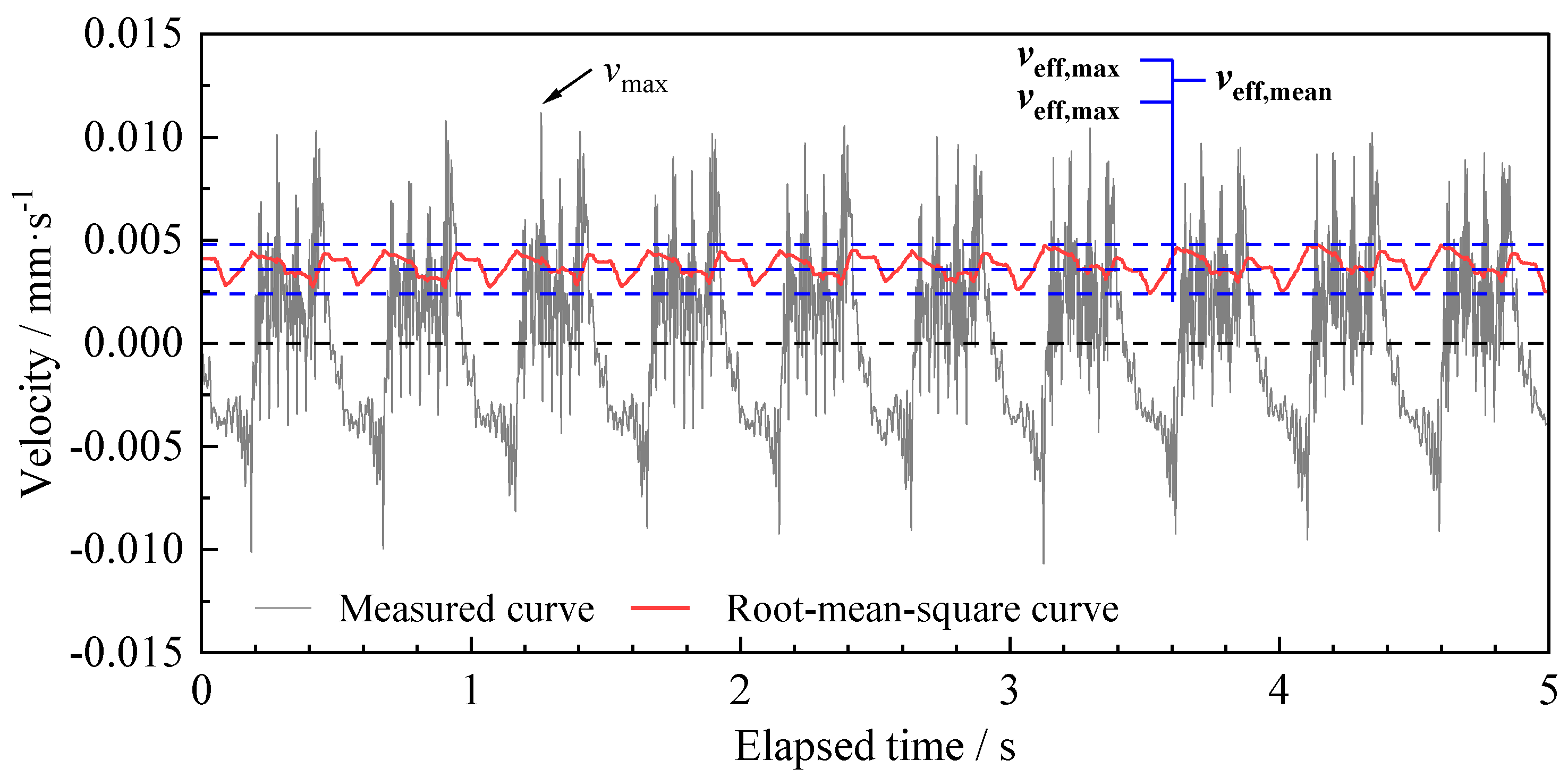
3.2. Vibration Velocity

As shown in Figure 9, the measured velocity−time curve oscillates between positive and negative throughout the train passage. The change in instantaneous values is rapid, barely reflecting the effect of vibrations on the long-term stability of railway earth structures. Based on the raw data of velocities, a root-mean-square (RMS) velocity with 0.125 s (fast window) was calculated and the results of effective velocities (veff) varying with time are shown in Figure 9. Using 100 km/h as an example, the veff value fluctuates on the positive side. The mean effective velocity (veff,mean) is approximately one-third of the peak value of the measured velocity, in line with the observations reported in the trial sections of the Waghäusel Saalbach–Graben–Neudorf railway [41] and the Wuhan–Guangzhou high-speed railway [42]. Note that the last two rail lines constructed were ballastless.
The maximum (veff,max), mean (veff,mean), and minimum values (veff,min) of the effective velocities are plotted against the train speed (V) in Figure 10. The three indicators of veff all increase linearly with increasing train speed. The veff,max peaks (4.58 mm/s) at 100 km/h. Using linear regression analysis, we determined the slope for each statistical indicator: kveff,max = 4.45%, kveff,mean = 3.51%, and kveff,min = 2.58% for the maximum, mean, and minimum values, respectively.
The German code for railway subgrade (DS 836-1997) [43] provides design values of effective velocity as a reference from different rail lines [41]. When ICE high-speed trains run at a speed of 300 km/h, the veff measured at the base of sleepers on ballasted tracks falls within 21 to 39 mm/s, and this value decreases to 12 to 21 mm/s on top of the concrete base in ballastless tracks. The equivalent vibration velocity of the roadbed surface should be controlled at 17.64 mm/s for ballasted track and 11.30 mm/s for ballastless tracks [41]. The published test data mentioned above could be used as a reference and comparison for this monitoring project. In the Hanover–Würzburg high-speed railway, which uses ballasted tracks, the veff reaches 18 to 20 mm/s at a depth of 0.7 m from the rail top with an operating speed of 250 km/h. The Nuremberg–Ingolstadt high-speed railway line, constructed with ballastless tracks, produces veff < 5 mm/s in the roadbed at V = 297 km/h; in addition, veff < 3 mm/s in the roadbed for V = 140–326 km/h, as observed in Schnellfahrstrecke Köln–Rhein/Main.
Although Chinese railways do not use train-induced velocity as a design index, some relevant field tests have been performed to examine the vibration velocities in the track foundation. When passenger and freight trains traveled at 19–93 km/h on the Guiyang–Kunming railway [44], the mean maximum velocities over the roadbed were reported to vary between 13 mm/s and 21 mm/s. In the Wuhan–Guangzhou high-speed railway [42], the mean peak velocities in the earth structure were below 10.15 mm/s (veff,max = 3.99 mm/s) as trains ran on ballastless track at 200–350 km/h. As prescribed in the Safety Technical Specification for Blasting Vibration of Railway Engineering (TB 10313-2019), the maximum particle velocity of blasting vibrations at the roadbed shoulder is used an indicator when assessing blasting impact. At frequencies less than 50 Hz, the allowable vibration velocity is lower than 50–70 mm/s for ballasted tracks and 30–50 mm/s for ballastless tracks. The monitoring results show that the calculated veff values of the instrumented section in the Watang–Rizhao railway are less than those in the German ballasted railway tracks and comparable to those from ballastless tracks. Using the equation vmax = 3·veff,mean to estimate the value of vmax, the derived vmax is smaller than those from the Guiyang–Kunming railway and slightly higher than the test results on the Wuhan–Guangzhou high-speed railway. Comparing against the requirement imposed by Code TB 10313−2019, the vmax values are comfortably below the limit values.
Based on the theory of shear wave propagation, the dynamic shear strain of soil can be obtained by:
γ = v eff / c s
where cs denotes the shear wave velocity. Vucetic [45] classified the soil response with linear cyclic threshold shear strain γ tl and volumetric cyclic threshold shear strain γ tv based on a statistical analysis of the results of laboratory tests on a large number of different soils under dynamic or cyclic loading. If the cyclic strain is below γ tl , the embankment fill essentially behaves as a linearly elastic medium, and the earth structure maintains stability under long-term dynamic loading. For cyclic strain between γ tl and γ tv , soil behavior becomes nonlinear, with the roadbed fill remaining stable under short-term loading but prone to failure under longer-term loading. For cyclic strain above γ tv , the soil response is more nonlinear and inelastic, and the embankment can fail under dynamic loading.
For coarse fills, γ tl = 3.5 × 10 6 ; the lower limit of γ tv is 5 × 10 5 and the mean 1.3 × 10 4 , denoted by γ tv , U and γ tv , M , respectively [41]. With cs set at 220 m/s [41], the values of dynamic shear strain calculated from Equation (5) are plotted against the operating speed in Figure 11. The γ value increases at higher operating speeds; for a speed range of 60 km/h to 100 km/h, the minimum value of γ min = 5.55 × 10 6 is higher than γtl. In contrast, the maximum value of γ max = 2.08 × 10 5 is lower than γtv,U.

3.3. Wheel–Rail Contact Force

In Figure 12, the time histories of the wheel–rail contact force are shown for quasi-static conditions (5 km/h) and dynamic conditions (taking the measured maximum speed 100 km/h as an example). A band-stop filter was used to filter out interference caused by the AC power source in China, which operates at 50 Hz. Considering the long length of the train, a representative window of six car passages is shown here, corresponding to 5 pairs of bogies. The contact force of each wheel–rail axle can be identified from the time signals, and each car contains four axles corresponding to four pulses. For an open wagon with a vehicle axle load of 30 t, the theoretical wheel–rail contact force is 150 kN.
The peaks of the measured data in Figure 12a fluctuate at approximately 150 kN, which indicates that the measurement is within the anticipated range. Compared to the lower speed, the peak values become more prominent at higher speeds due to rail surface roughness, track support stiffness, and track irregularities. In contrast to the 5 km/h signal, the 100 km/h signal exhibits a baseline drift (essentially a DC bias on the circuit), as shown in Figure 12b; this is consistent with the other field observations [46]. The strain gauges were deemed to be responsible for the observed phenomenon, i.e., the high frequencies caused by high speeds contributed to bias and drift in the measurement. Instead, peak-to-peak values were taken as dynamic wheel–rail contact forces.
The nominal axle load is usually measured under static conditions. However, for the design of railway tracks, it is necessary to determine the actual stresses in various track structure components and the rolling stock by using the dynamic forces imposed by a moving design vehicle at certain speeds (Figure 13a). The primary method of determining the design vertical wheel load is to express it as an empirical function of the static wheel load, given by:
P d = K d × P s
where Pd is the dynamic wheel load, kN; Kd > 1 is the dynamic impact factor; and Ps is the static wheel load, kN. An overview of the recommended expressions of Kd in various references is presented in Table 3. The number of factors is considered in the formula according to the quality and amount of track instrumentation and assumptions made concerning various related parameters.
The wheel–rail contact force distributions under different train speeds are plotted in Figure 13a, where the 95th and 99th percentiles are marked. A range of 125 kN to 165 kN is observed for the quasi-static condition, and the distribution range widens as the train speed increases, as also confirmed by the 95th and 99th percentiles. The measured forces usually range between 140 kN and 240 kN at 100 km/h. The wheel–rail contact forces at low speeds are relatively concentrated. In contrast, those at high speeds are relatively dispersed, indicating that train speed significantly affects the dispersion of the observed data. This pattern can be attributed to the combined action of track irregularities and high operating speed [50]. The measured values of the contact force are compared with the design values obtained by the approaches described in Table 3 and are shown in Figure 13b. The DZ4-type bogie is used in C96-type freight cars, with the diameter of the wheel (D) being 915 mm. A statistical analysis of the reported track modulus (k) reveals that k falls between 8 MPa and 34 MPa [51] but is mostly above 20 kPa. The value of k is prescribed as 25 MPa in this study. In the absence of detailed parameters for α , β , and γ , Equation (7) is introduced as a replacement for the formulae in Table 3, as recommended by the Union of Railways (UIC):
K d = 1.26 + 0.08 × ( V 100 ) 2
where V denotes the velocity in km/h. According to the comparison in Figure 13b, especially at 100 km/h, it is concluded that the design values recommended by China are the largest, while those from WMATA are the smallest; the UIC design values fall in between. The contact forces collected from the Watang−Rizhao heavy-haul railway increase at higher train speeds, yielding a maximum value of 238.7 kN and a mean of 184.1 kN at 100 km/h. The measured Kd can be expressed as a function of train speed:
K d = 1 + 0.46 V / 100
where V denotes the velocity in km/h. All the maximum values in different speed conditions are less than the design values recommended in China, indicating that the design of railway tracks incorporates a margin of safety.

4. Numerical Modelling

This section develops a 3D numerical model for the embankment-retaining wall system under test using the finite difference method (FDM). The model is configured to reflect the field conditions and validated using monitoring data. Further insight is gained by examining the quasi-static response of the embankment, for which limited field data were collected to perform a comprehensive structural serviceability assessment.

4.1. Model Development

The commercial software FLAC3D is utilized to establish a model depicting a ballasted track-embankment system supported by a retaining wall-ground (Figure 14). The model consists of beam structural elements that simulate the steel rails, and zone elements that represent the sleeper, and other structures below. The model comprises 483,630 elements and 507,523 grid points. Notably, 60 kg/m rail has moment of inertia Ix = 3217 cm4 about the horizontal axis, Iy = 524 cm4 about the vertical axis, and cross-sectional area A = 77.45 cm2. Furthermore, fasteners simulated by 100 kN/mm stiffness springs are placed between the rail and sleeper. In the model, the sleeper, ballast, and concrete retaining wall are considered as line elastomers, while the Mohr-Coulomb model is used for the roadbed, subgrade, and ground soil. The material parameters are presented in Appendix A. The wall–soil interaction is simulated by interfacial elements, whereby the normal stiffness kn and tangential stiffness ks is 40 GPa/m. The strength adheres to Coulomb’s criterion, with a friction angle at the wall–soil interface of 17.5°, while for other parts, this value is 21°. Roller boundaries are employed for the lateral sides, and pinned boundaries are used for the base of the model.
Our numerical simulation covers the entire construction process in four phases. First, the ground model is established, and the geostatic stress field is generated in the site preparation phase. The second phase involves constructing the retaining wall and placing backfill, followed by setting displacement and velocity fields to zero after convergence. The third phase simulates placing track structures and calculating the stress field. Finally, the railway structure’s quasi-static responses are obtained by applying field-instrumented train loads.
The model involves simulating the loads of two bogies adjacent to the front and rear freight cars. The measured wheel−rail contact forces are used as inputs in Equation (9), which is derived from Equations (6) and (8). Two scenarios are considered as shown in Figure 15:
(1)
Four-axle loading is symmetrically distributed along both sides of the sleepers on the center cross-section of the model (Loading position I)
(2)
The second axle of the four-axle loads is acting directly at the central cross-section of the model (Loading position II)
P d = 150 + 0.69 V
where P d and V are expressed in kN and km/h, respectively.

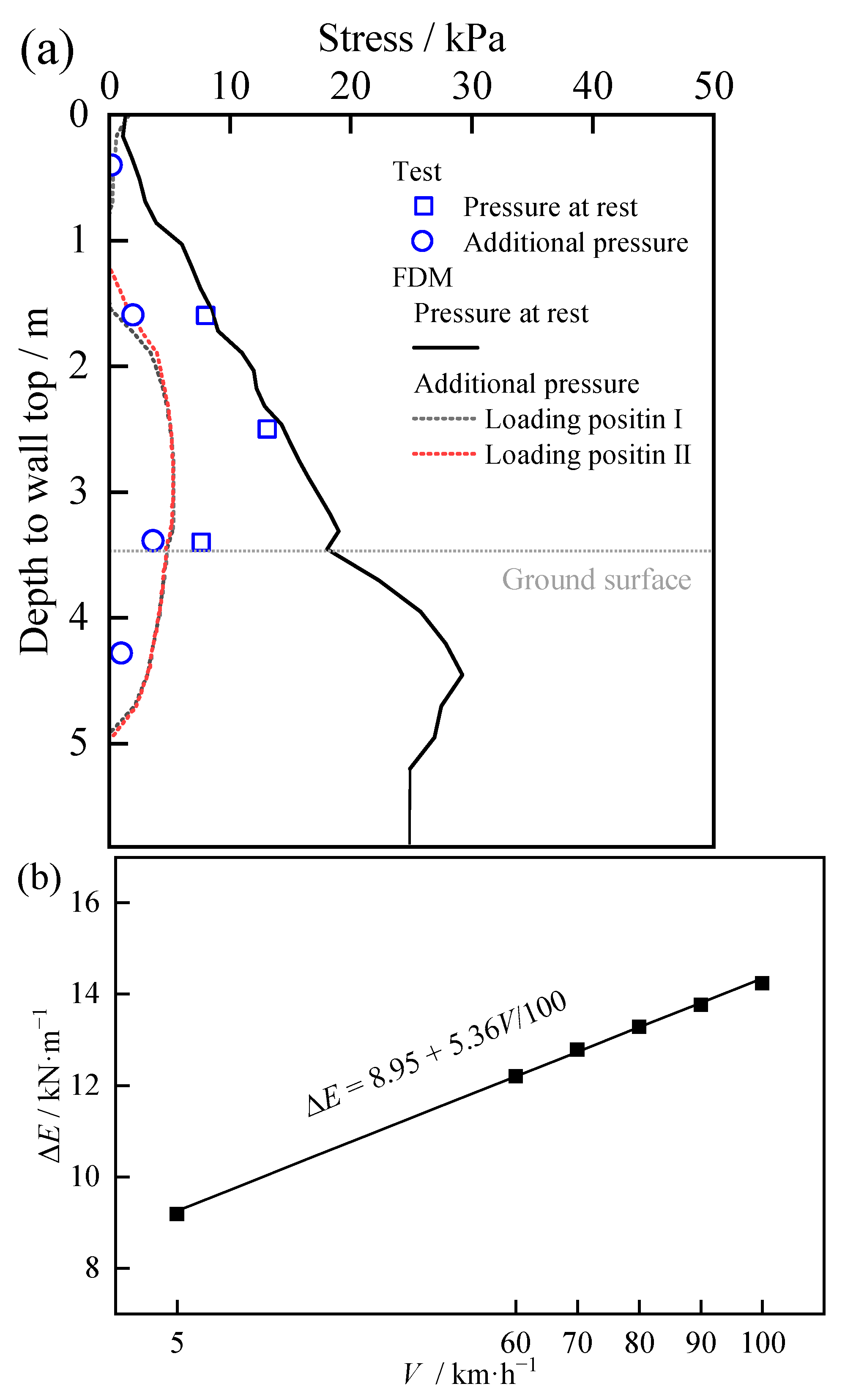
4.2. Analysis of Roadbed and Retaining Wall

Figure 15 illustrates the stress and displacement distribution of the roadbed surface beneath the near-wall side rail resulting from the train load at a velocity of 100 km/h. The peak values obtained from the FDM calculation are found to be essentially consistent with the tested data. As can be observed from Figure 15a, the peak stress generated by the four-axle loading on the roadbed surface is located beneath the sleeper, and the axle load placed directly above the rail sleeper results in a greater stress value. In comparison to the stress distribution, the fluctuation of displacement on the roadbed surface in Figure 15b is less pronounced, but the maximum value still occurs beneath the sleeper with the axle load acting directly above. Note that the train load predominantly impacts the soil within the roadbed structure. Consequently, the outcomes of roadbed surface displacement from FDM do not take into account the soil settlement underneath the roadbed [52].
The relationship between the maximum stress and displacement caused by train load on the roadbed surface below the rails and train speed V is presented in Figure 16. The FDM values and the field-tested data both suggest that an increase in V is not conducive to controlling quasi-static stress and displacement response on the roadbed surface. Our analysis of the simulation data reveals that the maximum stress σ rs and displacement s rs on the roadbed surface are linearly correlated with V, as expressed by Equations (10) and (11), respectively. This linear fit implies that the maximum stress and displacement on the roadbed surface induced by train passage can be estimated using the operating speed.
σ rs = 63.15 + 0.29 V
s rs = 0.45 + 0.22 V / 100
where σ rs , s rs , and V are expressed in kPa, mm, and km/h, respectively.
Figure 17 shows the distribution of earth pressure at the wall back and the variations in resultant force ΔE of the additional earth pressure induced by the train load with operating speed. As shown in Figure 17a, the FDM and test values [53] of earth pressure at rest against the wall without train traffic are in good agreement above the ground level, with slight deviations near the ground level. The additional earth pressure on the central cross-section of the model is minimally impacted by the loading position, with the calculated and measured values being roughly identical. An analysis of the FDM data indicates that the earth pressure at rest first increases linearly from top to bottom along the wall back and then decreases. The additional earth pressure is primarily distributed within a range of 1.5 m to 5.0 m from the wall top, increasing non-linearly and subsequently decreasing as the elevation decreases. Connecting the upper boundary of the additional earth pressure distribution range and the edge of the sleeper close to the wall, the angle between this connection line and the vertical direction is approximately 67.6°, and the corresponding angle of the lower boundary is approximately 42.3°. As shown in Figure 17b, the resultant force ΔE of additional earth pressure at the central cross-section of the model increases linearly with increasing speed, as expressed by:
Δ E = 8.95 + 5.36 V / 100
where Δ E and V are given in kN and km/h.
Figure 18 displays the horizontal displacement of the retaining wall due to train loading. Upon comparing Figure 18a,b, it is evident that the most significant horizontal displacement of the retaining wall transpires at the longitudinal center section of the four-axle load as the freight train travels through the embankment supported by a retaining wall. The horizontal displacement at the wall top resulting from the center of the four-axle load acting on the central cross-section (Loading position I) is greater than that at the base, as observed in Figure 18a. In contrast, Figure 18b shows that when the second axle of the four-axle load patten is at the central cross-section (Loading position II), the displacement of the wall base is marginally larger than that at the top of the wall. Furthermore, Figure 18c presents the variations in the horizontal displacement of the wall on the central cross-section of the entire FDM model with operating speed, revealing that the higher the speed of train operation, the greater the movement of the wall. For the load located in Loading position I, the displacement of the top of the wall at 100 km/h is 60.5% higher than that at 5 km/h and 20.6% higher than that at 60 km/h.

5. Conclusions

The magnitude of dynamic stresses propagating through railway retaining walls can be difficult to quantify at the design stage. Therefore, these retaining wall structures are often designed with a factor of safety that is higher than required. This results in an unnecessary increase in material usage, reducing the sustainability of the structure. To investigate the structure dynamics, this paper employed a field monitoring campaign to analyze the vibration response of a railway earth embankment with a retaining structure. The response of the structure to 30-ton axle load trains traveling at speeds of 5–100 km/h was studied. A three-dimensional FDM model was established to gain deeper insights into the response of the embankment-retaining wall system, in particular, the stress and displacement behaviors of the wall under train loads. The behavior of the rail infrastructure can be summarized as follows:
(1)
The maximum vibration acceleration values were 8.41 m/s2 and 4.93 m/s2 for the sleeper and roadbed, meeting the requirements for dynamic acceptance. At speeds 60 km/h, the PPA on the retaining wall was two orders lower than those on the sleeper and roadbed, and the sleeper was 1.7 times greater than that on the roadbed. For the same conditions, the PPA was between 4–5 times greater than the MTVV.
(2)
The spectrum amplitude attenuated along the propagation path, sleeper−subgrade−retaining structure, where the maximum VALs were 114.37 dB, 112.41 dB, and 77.42 dB. The sleeper and roadbed shared a similar distribution pattern, differing from the retaining wall. Material properties were observed to contribute more to the transmission of vibrations in substructures than speed.
(3)
The maximum effective velocity on the roadbed surface reached 4.58 mm/s at 100 km/h, and its slope was 4.45%. The maximum value of the shear strain was lower than the volumetric cyclic threshold shear strain, ensuring the long-term dynamic stability of the track formation.
(4)
The measured contact forces increased at higher train speeds, yielding a maximum value of 238.7 kN at 100 km/h, thus meeting the design requirements. The dynamic impact factor derived from the field test had the relationship, Kd = 1 + 0.46 V/100.
(5)
The application of train loads intensified the stress and displacement on the roadbed surface and created additional earth pressure on the retaining wall, resulting in horizontal wall movement. Notably, the earth pressure increased non-linearly before reaching its peak, after which it decreased as the elevation declined.

Author Contributions

Formal analysis, G.F. and P.L.; Investigation, G.F.; Writing—original draft, G.F. and P.L.; Writing—review & editing, D.P.C. and T.W.; Visualization, G.F. and P.L.; Supervision, Q.L., D.P.C. and T.W.; Project administration, Q.L.; Funding acquisition, Q.L., D.P.C. and T.W. All authors have read and agreed to the published version of the manuscript.

Funding

This study was supported by the National Natural Science Foundation of China (Grant No. 52078435), the Natural Science Foundation of Sichuan Province (Grant Nos. 2023NSFSC0391 and 2022NSFSC0404), the Royal Society (Grant No. IEC\NSFC\211306 - International Exchanges 2021 Cost Share), and the 111 Project (Grant No. B21011).

Data Availability Statement

The raw data for acceleration analysis is available via doi.org/10.6084/m9.figshare.21946421.

Conflicts of Interest

The authors declare no conflict of interest.

Appendix A

The construction and geotechnical material properties of the railway embankment and retaining wall in FDM modelling are shown in Table A1.
Table A1. Material property values used for FDM analysis.
ComponentDensity
(kg∙m−3)
Elastic Modulus
(MPa)
Poisson’s RatioCohesion
(kPa)
Friction Angle
(°)
Dilation Angle
(°)
Retaining wall230028,0000.20
Rail7830210,0000.30
Sleeper250036,0000.20
Ballast bed21303000.30
Roadbed (upper portion)2100241.40.25041.820.9
Roadbed (lower portion)2050190.80.30035.017.5
Subgrade2000166.80.30034.517.25
Ground1800138.60.3415.029.014.5
Compacted earth1900167.70.3039.035.017.5

References

  1. Kish, A. Guidelines to Best Practices for Heavy Haul Railway Operations–Infrastructure Construction and Maintenance Issues; International Heavy Haul Associations: Virginia Beach, VA, USA, 2009. [Google Scholar]
  2. Connolly, D.P.; Dong, K.; Alves Costa, P.; Soares, P.; Woodward, P.K. High Speed Railway Ground Dynamics: A Multi-Model Analysis. Int. J. Rail Transp. 2020, 8, 324–346. [Google Scholar] [CrossRef]
  3. Fernández-Ruiz, J.; Castanheira-Pinto, A.; Costa, P.A.; Connolly, D.P. Influence of Non-Linear Soil Properties on Railway Critical Speed. Constr. Build. Mater. 2022, 335, 127485. [Google Scholar] [CrossRef]
  4. Hu, J.; Bian, X. Analysis of Dynamic Stresses in Ballasted Railway Track Due to Train Passages at High Speeds. J. Zhejiang Univ. Sci. A 2022, 23, 443–457. [Google Scholar] [CrossRef]
  5. Lazorenko, G.; Kasprzhitskii, A.; Khakiev, Z.; Yavna, V. Dynamic Behavior and Stability of Soil Foundation in Heavy Haul Railway Tracks: A Review. Constr. Build. Mater. 2019, 205, 111–136. [Google Scholar] [CrossRef]
  6. Shan, Y.; Zhou, S.; Wang, B.; Ho, C.L. Differential Settlement Prediction of Ballasted Tracks in Bridge–Embankment Transition Zones. J. Geotech. Geoenviron. Eng. 2020, 146, 04020075. [Google Scholar] [CrossRef]
  7. Charoenwong, C.; Connolly, D.P.; Odolinski, K.; Alves Costa, P.; Galvín, P.; Smith, A. The Effect of Rolling Stock Characteristics on Differential Railway Track Settlement: An Engineering-Economic Model. Transp. Geotech. 2022, 37, 100845. [Google Scholar] [CrossRef]
  8. Nie, R.; Sun, B.; Leng, W.; Li, Y.; Ruan, B. Resilient Modulus of Coarse-Grained Subgrade Soil for Heavy-Haul Railway: An Experimental Study. Soil Dyn. Earthq. Eng. 2021, 150, 106959. [Google Scholar] [CrossRef]
  9. Chen, X.; Nie, R.; Li, Y.; Guo, Y.; Dong, J. Resilient Modulus of Fine-Grained Subgrade Soil Considering Load Interval: An Experimental Study. Soil Dyn. Earthq. Eng. 2021, 142, 106558. [Google Scholar] [CrossRef]
  10. Wang, T.; Luo, Q.; Liu, J.; Liu, G.; Xie, H. Method for Slab Track Substructure Design at a Speed of 400 Km/h. Transp. Geotech. 2020, 24, 100391. [Google Scholar] [CrossRef]
  11. Xie, H.; Luo, Q.; Wang, T.; Jiang, L.; Connolly, D.P. Stochastic Analysis of Dynamic Stress Amplification Factors for Slab Track Foundations. Int. J. Rail Transp. 2023, 1–23. [Google Scholar] [CrossRef]
  12. Shan, Y.; Shu, Y.; Zhou, S. Finite-Infinite Element Coupled Analysis on the Influence of Material Parameters on the Dynamic Properties of Transition Zones. Constr. Build. Mater. 2017, 148, 548–558. [Google Scholar] [CrossRef]
  13. Luo, Q.; Fu, H.; Liu, K.; Wang, T.; Feng, G. Monitoring of Train-Induced Responses at Asphalt Support Layer of a High-Speed Ballasted Track. Constr. Build. Mater. 2021, 298, 123909. [Google Scholar] [CrossRef]
  14. Xia, F.; Cole, C.; Wolfs, P. The Dynamic Wheel– Rail Contact Stresses for Wagon on Various Tracks. Wear 2008, 265, 1549–1555. [Google Scholar] [CrossRef]
  15. Zhai, W.; Wang, K.; Lin, J. Modelling and Experiment of Railway Ballast Vibrations. J. Sound Vib. 2004, 270, 673–683. [Google Scholar] [CrossRef]
  16. Wang, T.; Luo, Q.; Zhang, L.; Xiao, S.; Fu, H. Dynamic Response of Stabilized Cinder Subgrade during Train Passage. Constr. Build. Mater. 2021, 270, 121370. [Google Scholar] [CrossRef]
  17. Zhai, W.; Wang, Q.; Lu, Z.; Wu, X. Dynamic Effects of Vehicles on Tracks in the Case of Raising Train Speeds. Proc. Inst. Mech. Eng. Part F J. Rail Rapid Transit 2001, 215, 125–135. [Google Scholar] [CrossRef]
  18. Sheng, X.; Jones, C.J.C.; Thompson, D.J. A Comparison of a Theoretical Model for Quasi-Statically and Dynamically Induced Environmental Vibration from Trains with Measurements. J. Sound Vib. 2003, 267, 621–635. [Google Scholar] [CrossRef]
  19. Milne, D.R.M.; Le Pen, L.M.; Thompson, D.J.; Powrie, W. Properties of Train Load Frequencies and Their Applications. J. Sound Vib. 2017, 397, 123–140. [Google Scholar] [CrossRef]
  20. Di, H.; Yu, J.; Guo, H.; Zhou, S.; He, C.; Zhang, X. Modeling of Ground Vibrations from a Tunnel in Layered Unsaturated Soil with Spatial Variability. Arch. Civ. Mech. Eng. 2022, 22, 33. [Google Scholar] [CrossRef]
  21. Auersch, L.; Said, S. Dynamic Track-Soil Interaction—Calculations and Measurements of Slab and Ballast Tracks. J. Zhejiang Univ. Sci. A 2021, 22, 21–36. [Google Scholar] [CrossRef]
  22. Dong, J.; Yang, Y.; Wu, Z.-H. Propagation Characteristics of Vibrations Induced by Heavy-Haul Trains in a Loess Area of the North China Plains. J. Vib. Control 2019, 25, 882–894. [Google Scholar] [CrossRef]
  23. Ren, J.; Wang, J.; Li, X.; Wei, K.; Li, H.; Deng, S. Influence of Cement Asphalt Mortar Debonding on the Damage Distribution and Mechanical Responses of CRTS I Prefabricated Slab. Constr. Build. Mater. 2020, 230, 116995. [Google Scholar] [CrossRef]
  24. Deng, S.; Ren, J.; Wei, K.; Ye, W.; Du, W.; Zhang, K. Fatigue Damage Evolution Analysis of the CA Mortar of Ballastless Tracks via Damage Mechanics-Finite Element Full-Couple Method. Constr. Build. Mater. 2021, 295, 123679. [Google Scholar] [CrossRef]
  25. Auersch, L. The Excitation of Ground Vibration by Rail Traffic: Theory of Vehicle–Track–Soil Interaction and Measurements on High-Speed Lines. J. Sound Vib. 2005, 284, 103–132. [Google Scholar] [CrossRef]
  26. Mei, H.; Leng, W.; Nie, R.; Liu, W.; Chen, C.; Wu, X. Random Distribution Characteristics of Peak Dynamic Stress on the Subgrade Surface of Heavy-Haul Railways Considering Track Irregularities. Soil Dyn. Earthq. Eng. 2019, 116, 205–214. [Google Scholar] [CrossRef]
  27. Ye, Q.; Luo, Q.; Connolly, D.P.; Wang, T.; Xie, H.; Ding, H. The Effect of Asphaltic Support Layers on Slab Track Dynamics. Soil Dyn. Earthq. Eng. 2023, 166, 107771. [Google Scholar] [CrossRef]
  28. Beben, D.; Anigacz, W.; Ukleja, J. Diagnosis of Bedrock Course and Retaining Wall Using GPR. NDT E Int. 2013, 59, 77–85. [Google Scholar] [CrossRef]
  29. Bian, X.; Chao, C.; Jin, W.; Chen, Y. A 2.5 D Finite Element Approach for Predicting Ground Vibrations Generated by Vertical Track Irregularities. J. Zhejiang Univ. Sci. A 2011, 12, 885–894. [Google Scholar] [CrossRef]
  30. Yang, G.; Zhang, B.; Lv, P.; Zhou, Q. Behaviour of Geogrid Reinforced Soil Retaining Wall with Concrete-Rigid Facing. Geotext. Geomembr. 2009, 27, 350–356. [Google Scholar] [CrossRef]
  31. Esen, A.F.; Woodward, P.K.; Laghrouche, O.; Čebašek, T.M.; Brennan, A.J.; Robinson, S.; Connolly, D.P. Full-Scale Laboratory Testing of a Geosynthetically Reinforced Soil Railway Structure. Transp. Geotech. 2021, 28, 100526. [Google Scholar] [CrossRef]
  32. Zhu, S.; Wu, L.; Song, X. An Improved Matrix Split-Iteration Method for Analyzing Underground Water Flow. Eng. Comput. 2022. [Google Scholar] [CrossRef]
  33. The National Railway Administration (NRA). Code for Design of Retaining Structure of Railway Earthworks (TB 10025-2019); China Railway Publishing House Co., Ltd.: Beijing, China, 2019. [Google Scholar]
  34. The National Railway Administration (NRA). Code for Design of Railway Earth Structure (TB 10001-2016); China Railway Publishing House Co., Ltd.: Beijing, China, 2016. [Google Scholar]
  35. The National Railway Administration (NRA). Code for Design of Railway Track (TB 10082-2017); China Railway Publishing House Co., Ltd.: Beijing, China, 2017. [Google Scholar]
  36. ISO 2631-1; Mechanical vibration and shock — Evaluation of human exposure to whole-body vibration — Part 1: General requirements. ISO: Geneva, Switzerland, 1997.
  37. Feng, G.; Wang, T. Raw_acceleration_data.xlsx. 2023. Available online: https://figshare.com/articles/dataset/Raw_acceleration_data_xlsx/21946421 (accessed on 24 January 2023).
  38. Kouroussis, G.; Verlinden, O.; Conti, C. Free Field Vibrations Caused by High-Speed Lines: Measurement and Time Domain Simulation. Soil Dyn. Earthq. Eng. 2011, 31, 692–707. [Google Scholar] [CrossRef]
  39. The National Railway Administration (NRA). Technical Regulations for Dynamic Acceptance for Mixed Passenger and Freight Railways Construction (TB 10461-2019). China Railway Publishing House Co., Ltd.: Beijing, China, 2019. [Google Scholar]
  40. Chen, C.; Chang, L.; Loh, C. A Review of Spectral Analysis for Low-Frequency Transient Vibrations. J. Low Freq. Noise Vib. Act. Control 2021, 40, 656–671. [Google Scholar] [CrossRef]
  41. Hu, Y.; Li, N. Theory of Ballastless Track-Subgrade for High Speed Railway, 1st ed.; China Railway Publishing House: Beijing, China, 2010; ISBN 978-7-113-11729-0. [Google Scholar]
  42. Qu, C.; Kang, K.; Wei, L.; Guo, K.; He, Q. Dynamic Response Characteristics and Long-Term Dynamic Stability of Subgrade-Culvert Transition Zone in High-Speed Railway. Rock Soil Mech. 2020, 41, 3432–3442. [Google Scholar]
  43. DS 836-1997; Tilbagetrukket. Havebrugsmaskiner. Motoriserede plæneklippere. Sikkerhed. Dansk: Mount Kisco, NY, USA, 1998.
  44. Xiao, G. Test Study on Railway Subgrade Reinforced by Sand Compacted Pile and Geocell. Master’s thesis, Southwest Jiaotong University, Chengdu, China, 2005. [Google Scholar]
  45. Vucetic, M. Cyclic Threshold Shear Strains in Soils. J. Geotech. Eng. 1994, 120, 2208–2228. [Google Scholar] [CrossRef]
  46. Sarikavak, Y.; Goda, K. Dynamic Wheel/Rail Interactions for High-Speed Trains on a Ballasted Track. J. Mech. Sci. Technol. 2022, 36, 689–698. [Google Scholar] [CrossRef]
  47. Liang, C.; Si, D.; Liu, H. Comparative Analysis of Dynamic Load Coefficient of Railway Track Structures at Home and Abroad. Railw. Eng. 2021, 61, 100–103. [Google Scholar] [CrossRef]
  48. Choi, J.; Yun, S.; Chung, J.; Kim, S. Comparative Study of Wheel–Rail Contact Impact Force for Jointed Rail and Continuous Welded Rail on Light-Rail Transit. Appl. Sci. 2020, 10, 2299. [Google Scholar] [CrossRef]
  49. Doyle, N.F. Railway Track Design: A Review of Current Practice; Australian Government Publishing Service: Canberra, Australia, 1980; ISBN 0-642-05014-7. [Google Scholar]
  50. Eisenmann, J. Germans Gain a Better Understanding of Track Structure. Railw. Gaz. Int. 1972, 128, 305–308. [Google Scholar]
  51. Bose, T.; Levenberg, E. A Priori Determination of Track Modulus Based on Elastic Solutions. KSCE J. Civ. Eng. 2020, 24, 2939–2948. [Google Scholar] [CrossRef]
  52. Wang, F.; Qi, J.; Du, J. Dynamic Deformation Analysis Method and Reliability on the Subgrade Surface of the High-Speed Ballast Track. J. Saf. Environ. 2016, 16, 144–149. [Google Scholar]
  53. Feng, G.; Zhang, L.; Luo, Q.; Wang, T.; Xie, H. Monitoring the Dynamic Response of Track Formation with Retaining Wall to Heavy-Haul Train Passage. Int. J. Rail Transp. 2022, 1–19. [Google Scholar] [CrossRef]
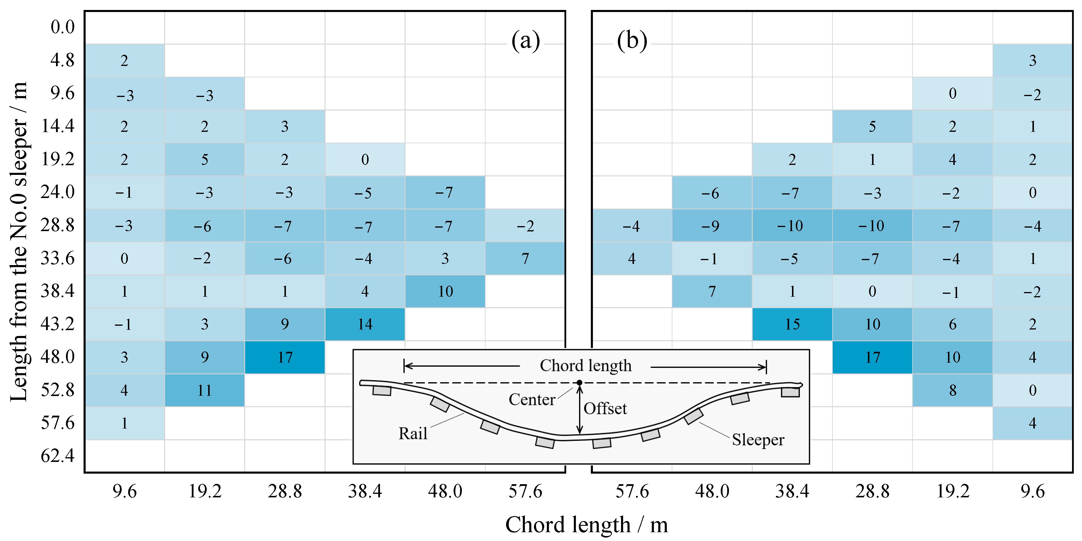
Figure 1. Route of the heavy-haul railway of interest and the field test section.
Sustainability 15 07984 g001
Figure 2. Cross-sectional view of the railway track, underlain by an embankment supported by a gravity retaining wall: K is the percentage of compaction for the embankment fill; two vibration sensors are placed on the roadbed surface.
Sustainability 15 07984 g002
Figure 3. Overview of the test site: (a) Gondola cars running through the study area; (b) a general view of the double-track railway.
Sustainability 15 07984 g003
Figure 4. Longitudinal level of the (a) left and (b) right rails against chord length. A darker color indicates a higher value.
Sustainability 15 07984 g004
Figure 5. Field instrumentation: (a) excavation of the ballast; (b) integrated vibration sensors over the roadbed surface; (c) data acquisition system; (d) rail grinding at predetermined locations; (e) strain gauges glued to the rail web; (f) calibration of strain gauges.
Sustainability 15 07984 g005
Figure 6. Configuration of (a) the locomotive and (b) the freight car, and key dimensions (c): La is the axle spacing within a bogie, Lb is the bogie spacing, Lc is the vehicle length, and Lr is the rail gauge.
Sustainability 15 07984 g006
Figure 7. Time histories (left) and frequency spectra (right) of accelerations on the (a) sleeper, (b) roadbed, and (c) retaining wall at 100 km/h. Shaded areas correspond to the amplitude peaks.
Sustainability 15 07984 g007
Figure 8. Transfer functions, (a) TFSR and (b) TFRW: TFSR, from sleeper to roadbed; TFRW, from roadbed to retaining wall (denoted by R-wall).
Sustainability 15 07984 g008
Figure 9. Comparison of the measured velocity−time curve and the root-mean-square values on the roadbed at 100 km/h.
Sustainability 15 07984 g009
Figure 10. Relationship between effective velocities on the roadbed surface and the train speed.
Sustainability 15 07984 g010
Figure 11. Dynamic shear strains of subgrade versus train speed: γ m a x , γ m i n , and γ m i n are the maximum, minimum, and mean values of the dynamic shear strain derived from statistical analysis.
Sustainability 15 07984 g011
Figure 12. Time histories of the wheel–rail vertical contact force for (a) quasi-static and (b) dynamic conditions (5 km/h and 100 km/h).
Sustainability 15 07984 g012
Figure 13. (a) Distribution of observed wheel–rail contact force and (b) comparison with the design values of Kd with D = 915 mm and k = 25 MPa. The symbol ‘S’ means the number of samples, and the subscript ‘obf’ in the fitting formulae denotes the observed force.
Sustainability 15 07984 g013
Figure 14. Configuration and meshes of the three-dimensional numerical model.
Sustainability 15 07984 g014
Figure 15. Stress (a) and displacement (b) distributions on roadbed surface under train loads.
Sustainability 15 07984 g015
Figure 16. The maximum (a) stress and (b) displacement on roadbed surface versus operating speed.
Sustainability 15 07984 g016
Figure 17. Earth pressure against the retaining wall at 100 km/h: (a) distribution along the elevation; (b) variations in additional earth pressure Δ E with operating speed V.
Sustainability 15 07984 g017
Figure 18. Horizontal movement of the retaining wall: (a) center of the four-axle load at the central cross-section; (b) second axle of the four-axle loads at the central cross-section; (c) displacement distributions varying with speed.
Sustainability 15 07984 g018
Table 1. Elevation readings of the rails and cross-level measurements.
ItemSleeper ID
081624324048566472808896104
LS0/m04.89.614.419.22428.833.638.443.24852.857.662.4
RL/mm277325376421469521571616661707752803861921
RR/mm297342393440489541593638684727773827881942
Cross level/mm0−3−3−10022301401
Note: LS0 denotes the length from the #0 sleeper; RL and RR are the elevation readings of the left and right rails obtained from the digital level; the negative value of the cross level indicates an elevation for the left rail higher than the right rail.
Table 2. Measured PPA and MTVV at different locations and speeds.
PPA/m·s−2
Sensor Location5 km/h60 km/h70 km/h80 km/h90 km/h100 km/h
Sleeper0.055.045.887.047.798.41
Subgrade surface0.033.043.543.974.494.93
Retaining wall top0.020.050.060.060.070.07
MTVV/m·s−2
Sensor Location5 km/h60 km/h70 km/h80 km/h90 km/h100 km/h
Sleeper0.021.051.301.441.872.07
Subgrade surface0.010.630.810.881.020.99
Retaining wall top0.000.020.020.030.030.04
Table 3. Empirical expressions to determine the value of dynamic impact factor Kd.
No.ReferenceRelationship
1The Office of Research and Experiments of the International Union of Railways (ORE, UIC) 1 + α + β + γ
2China [47] 1 + 0.6 V / 100
3Washington Metropolitan Area Transit Authority, U.S. (WMATA) ( 1 + 3.86 × 10 5 V 2 ) 0.67
4American Railway Engineering and Maintenance-of-Way Association (AREMA) 1 + 5.21 V / D
5Deutsche Bahn, Germany (DB) 1 + V 2 3 × 10 4
6Clarke, British 1 + 19.65 V D k
7Korean [48] 1 + 0.513 V / 100
8South African 1 + 4.92 V / D
9Indian 1 + V 58.14 k
Note: Unmarked references were obtained from [49]. V is the train speed in km/h; D is the wheel diameter in mm; k is the track modulus in MPa; and α , β , and γ are the parameters related to the track geometry, train speed, and rolling stock properties, respectively.
Disclaimer/Publisher’s Note: The statements, opinions and data contained in all publications are solely those of the individual author(s) and contributor(s) and not of MDPI and/or the editor(s). MDPI and/or the editor(s) disclaim responsibility for any injury to people or property resulting from any ideas, methods, instructions or products referred to in the content.

