Abstract
The quick development of industrial sectors, tourism, and agriculture, which coincided with human habitation in cities, has led to the degradation of environmental qualities. Thus, a detailed plan is required to balance the development and environmental conservation of urban areas to achieve sustainability. This paper uses the environmental carrying capacity (i.e., ecological footprint and biological capacity) model to estimate ecological sustainability and achieve the desired balance. The results reveal that problems, such as unbalanced land development, the destruction of protected areas, and changes in land use in favor of industrial and residential development, persist in the area under study. Additionally, the studied area has been facing an ecological deficit since 1992. If this trend continues, the area will lose its chance for ecological restoration by 2030, when the ecological deficit reaches −3,497,368 hectares. The most important indicators in the ecological footprint were resource consumption in industries, water consumption in agriculture, and pollution generation from industries and household consumption. Therefore, in a sustainable scenario, the ratio of these indicators was changed based on Alborz’s development policies. In order to achieve ecological balance in the study area, short-, medium-, and long-term scenarios were proposed, as follows: (a) preventing the ecological deficit from reaching the critical threshold by 2030, (b) maintaining the ecological deficit at the same level until 2043, and (c) bringing Alborz to ecological balance (bringing the ecological deficit to zero) by 2072.
1. Introduction
The growing rate of urbanization, together with its socio-environmental effects, are the main global challenges. The world’s urban population multiplied from 751 million in 1950 to 4.36 billion in 2020, and by 2030 this number is expected to rise to about 5 billion. The increasing levels of urbanization are linked to the reduction in natural reserves and soil degradation, a loss of biodiversity, and an increase in the pollution of land, water, and air [1], as short-term and intensive human activities lead to large numbers of organic pollutants, such as polyhalogenated compounds, along with inorganic pollutants, such as potentially toxic metals [2,3]. Higher levels of environmental deterioration are expected in the coming years due to the growth in the human population, especially in urban areas [4], because towns are assigning the carrying capacity of ecosystems outside their borders via trading food resources, services, and energy sources [5,6]. Based on Rees [7], the land, which is functionally occupied by city inhabitants’ demands, goes far beyond the city’s borders. The current rate of urban area growth indicates the importance of these areas as the center of sustainability assessments [8]. Therefore, there is a need to assess the state of balance and the boundaries to growth for the future development of human settlements [9]. Including the assessment of environmental carrying capacity (ECC) in cities’ spatial management and planning can be a useful tool for developing sustainable human settlements [10,11,12,13,14,15].
The environmental carrying capacity (ECC) has been used as an index of sustainable development, making it possible to quantitatively assess environmental and urban sustainability [16,17], and it is considered as a threshold level of anthropopressure, which the environment can balance and withstand without irreversible changes and severe degradation [18]. The ECC verifies whether the current spatial management is consistent or inconsistent with certain constraints on the environment and poses limits to the ability of current and future populations to satisfy their needs [19,20,21]. The essence of environmental carrying capacity is the comparison between supply and demand. One of the most frequently suggested remedies for ECC assessment is using environmental indicators, such as ecological footprint (EF) and biocapacity (BC) [18].
The ecological footprint concept is “estimating the land that is used to produce goods and services dedicated to meeting the final domestic demand of a city or country regardless of the area in which the land is actually used” [22]. This awareness generates a rising enthusiasm for computing methodologies to track the sustainable consumption of natural reserves [23,24,25]. The ecological footprint is a tool to convey the effect of resource consumption on the environment to the general public via a visual presentation. It can be used to increase public awareness, compensate for human pressures on the environment [26], and promote ecological civilization [17,27,28]. BC represents the actual annual bioproductive ability of an area (an ecological benchmark) to meet human needs. Thus, the BC assesses an actual annual ecosystem service budget available [29]. This is a key ingredient for all of humanity’s goods and services. BC measures the nature bioproductivity of a given area, which reflects the biosphere’s regenerative capacity [30,31] and provides ecosystem services, i.e., carbon dioxide sequestration [32]. The difference between the EF and BC could identify the state of the environment. If the EF is higher than BC, it represents the state of the environment called an ecological deficit; when the BC is higher than EF, the state of ecological reserve shows a higher nature bioproductivity than the demand for resources [33,34].
Many experts have conducted research on ECC. For instance, Liu et al. [1] quantitatively assessed the physical value of natural capital in China based on an EF model, the results of which show that between 2000 and 2018, physical quantities of the per capita EF and per-capita ED increased, while the physical quantity of per-capita ECC decreased. Long et al. [35] studied sustainability using a three-dimensional EF and human development index. The results show that the area faces an ED, and increasing the human development index by declining the EF can boost the efficiency of ecological resource use and help to obtain sustainable urban development in such areas. Wu et al. [36] investigated the sustainability and decoupling effects of natural capital use in China by also employing three-dimensional EF. The results demonstrate that an environmental surplus occurred in 2000, while all provinces were in a state of the ED in 2016. In addition, EF per capita rose because of the growth in croplands and settlement areas. Another study shows that growing settlement areas in Najaf, Iran, have enacted considerable pressure on natural resources that exceed the biological capacity of the land, especially its carbon footprint and energy footprint [37]. Xie et al. [38] showed the Shanghai port logistics ecosystem is still in an ecological deficit through the footprint of energy, pollution, and water. Rapid economic and population growth has led to continuous demand expansion for marine fishery resources [39]. The ecological deficit of marine fisheries shows an expanding trend due to the joint effect between marine fishery biological capacity and ecological footprint [40,41]. Ahmed and Weng [42] investigated human capital in India between 1971 and 2014 and its effect on the ecological footprint. The results showed a considerable negative contribution of human capital to the ecological footprint. Destek et al. [43] illustrated that the consumption of nonrenewable energy [44] increased environmental degradation, as well as ecological footprint, from 1980 to 2013 in the EU countries.
However, most of the papers explain the current status of the ECC and put less concentration on the dynamic changes of the ECC. As a result, there is less research on its anticipation, which makes it difficult to participate in regional development decision-making. Moreover, the current investigation of the ECC is mostly limited to the national level, and there are only a few studies on the sustainability of urban scales. In this study, the Alborz province was selected to implement the concept of the ECC for more sustainable spatial management. The research evaluates the spatial policy established by the city’s municipality and its surroundings and presents short-, medium-, and long-term plans to reduce the ecological footprint by 2072.
2. Materials and Methods
2.1. Study Area
Alborz Province (Figure 1), with an area of 5833 km2, is located in the west of Tehran (the capital of Iran) on the hills of the Alborz Mountains. Alborz Province is situated between latitudes 35°37′ and 36°50′ N and longitudes 50°24′ and 50°90′ E. The average elevation of Alborz Province is 2600 m. With a moderate climate, this area is considered one of the most important areas for agriculture and livestock in Iran [45,46]. The study area has been facing problems, such as strong immigration of people from the rural areas and the city center (Tehran), as well as the development of new residential housing and industrial areas on former grass- and agricultural lands.
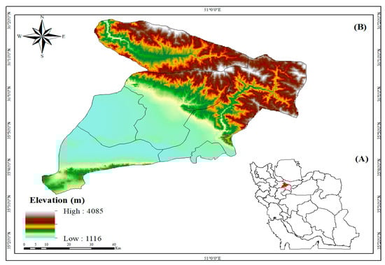
Figure 1.
Alborz Province (B) of Iran (A) is illustrated using a digital elevation model (DEM).
2.2. Assessment of Land Use/Land Cover Change (LULCC)
In this study, the CA-Markov model was used to predict and investigate LULCC. The CA-Markov model was used for both spatial and temporal changes and is one of the most frequently utilized techniques to quantitatively predict the dynamic changes in landscape patterns [47]. The CA-Markov model describes LULCC from one time period to another, and this is the basis used to project future changes [48,49]. The LULC maps were obtained from Earth Explorer, which are Landsat images (Table 1). The 2001, 2016, and 2022 datasets were used to develop LULC maps to identify change. Moreover, field visits were conducted at 86 random points to validate and correct the classification of the images, and after conforming to the LULC map, the coefficient of kappa and overall accuracy were 0.82 and 86%, respectively, in 2022 (Table 2). Finally, LULC was classified into eight classes using the maximum likelihood method, namely Fallow land, Garden, Bare land, Water body, Forest, Arable land, Grass land, and Settlement [50,51,52].

Table 1.
Landsat images.
Table 2.
Confusion matrix of 2022 land use/land cover.
2.3. Environmental Carrying Capacity (ECC)
The difference between the BC and EF allowed for the quantification of the ECC and the definition of the environment state, referred to as ecological deficit, ecological reserve, or ecological balance. The ecological deficit is a concept that describes how the region’s environment is exploited quantitatively. The amount of environmental deficit shows whether or not the area exceeded its biological capacity levels. An area can be described as a ‘deficit area’ when the ecological footprint exceeds its biological capacity [53]. In this study, the concept of ecological deficit was used to determine the sustainable economic structure [54]. The ecological deficit is the most common and most straightforward mathematical indicator with relative and ecological comparison goals. This index is much more efficient than other methods for calculating ecological sustainability. Indeed, the ecological deficit is an indicator for finding the optimal value of objective functions, which includes linear constraints based on variables (ecological footprint and biological capacity) [55,56].
where
ECC = Environmental carrying capacity;
BC = Biological capacity;
EF = Ecological footprint.
2.3.1. Biological Capacity
Biological capacity refers to the capacity of an ecosystem to produce useful vital substances sustainably and absorb the wastes that are produced by humans. Useful vital substances are those substances that are consumed by the human economy. The biological capacity of an area is calculated by multiplying the actual physical regions in the yield coefficient and the proper equilibrium coefficient [57].
where
A = level of each land use type in the area (hectares);
Yf = natural production coefficient for each land use type;
Eqf = equilibrium coefficient for each land use type.
It should be noted that man-made uses of ‘urban development’ and ‘infrastructure’ do not have the natural productive capacity, and their Eqf and Yf values are calculated from the weighted average of other land use types, whereby their values will only be effective in calculating the ecological footprint [30].
Production Coefficient
The production coefficient shows the production capacity of each land use type in comparison with the reference level in the study area. In this study, the reference level of the country is Iran, and the study area is Alborz Province [30].
where
Yf = production coefficient of each land use type in the study area;
Yr = (tons per hectare) the annual production of each land use type in the study area;
Yc = (tons per hectare) the amount of annual production of each land use type at the reference level (country).
Equilibrium Coefficient
The equilibrium coefficient illustrates the potential of global production for every land use type [30].
where
j = the type of resource consumption;
i = the productive use of the source i;
= the consumption of the source i in the use of the region j;
= the value of the source i in the use of the region j;
= the biological production of the use i.
Since the equilibrium coefficient (the potential of global production for every land use type) is a fixed and universal value, its values are available in Table 3 [30].
Table 3.
Equilibrium coefficient for each land use/land cover type.
2.3.2. Ecological Footprint
The ecological footprint is the demand of the people in an ecosystem. Biological capacity is nature’s ability to provide the reserves and ecosystem services that are consumed by humans annually [58]. The ecological footprint is a quantitative indicator for measuring the impact of human activities in the four major sectors of service, industry, agriculture, and home consumption on the biosphere. In the first step, annual consumption is estimated based on local, regional, or national data in each sector that is related to energy consumption, food, forests, and other goods. The next step involves estimating the land per capita allocated to production for each major consumption segment. This estimation is carried out by dividing a sector’s annual consumption by that sector’s average annual productivity. Next, the total ecological footprint is equal to the total land area allocated to all sectors consumed by all sectors in one year [59]. Overall, the ecological footprint determines the degree of unsustainability with the difference between available and required land. Unsustainable populations are those with a higher ecological footprint than available land [60].
where
EF = ecological footprint of the area;
= ecological footprint of resource consumption in the region;
= ecological footprint of energy consumption in the region;
= ecological footprint of waste generation in the region;
= ecological footprint of pollutant emissions in the region;
= amount of recycled material in the area.
where
= amount of consumption per resource in the area (tons);
= natural average production of land uses related to the source at the reference level (country) (tons per hectare);
= average natural balance coefficient of land uses associated with the source of consumption;
= average natural production coefficient of land uses related to the source of consumption.
where
= amount of energy consumption in the region (tons);
= average natural production of land uses related to the production of energy consumption at the reference level (tons per hectare);
= average natural equilibrium coefficient of land uses related to energy production;
= average natural production coefficient of land uses related to energy production.
where
= annual effluent generation of the region by category i industries (m3);
= amount of nationally programmable water for industries (m3 per hectare).
2.4. The ECC Forecasting Model
The R and ARIMA models were used to predict the EF and EC as an early warning of future ecological security. ARIMA, which stands for auto-regressive integrated moving average, is a foreseeing algorithm based on three parametric components, including autoregression (AR): a model that uses the dependent relationship between an observation and some number of lagged observations, integration (I): the use of differential raw observations (e.g., subtracting an observation from an observation at the previous time step) to make the time series stationary, and moving average (MA): a model that uses the dependency between an observation and a residual error from a moving average model applied to lagged observations [61,62].
where
= the differenced series;
ϕ1 = the coefficient of the first AR term;
p = the order of the AR term;
θ1 = the coefficient of the first MA term;
q = the order of the MA term;
εt = the error.
2.5. Data Sources
A huge amount of data on resource consumption was needed to calculate the EF and BC. So, a lot of information sources were reviewed from the published statistical yearbooks, development documents, web pages, governmental reports, statistical reports, and databases. In this paper, the primary consumption data relating to forestry, agriculture, aquatic goods, and energy consumption was directly gathered from the Iran Statistical Yearbooks, Statistical Yearbook of Fisheries, Statistical Yearbook Energy, e.g., ISY, 2009–2010, 2010–2011, 2011–2012, 2012–2013, 2013–2014, 2014–2015, 2015–2016, 2016–2017, 2017–2018, 2018–2019, 2019–2020, 2020–2021, 2021–2022, SYF 1999–2021, and SYE 1990–2021. Additionally, the data were provided by the Organization of Agriculture-Jahad-Alborz, the Ministry of Petroleum, and the Statistical Summary of Iran’s Electricity Industry [63,64,65,66,67,68,69]. In addition, to standardize the collected data, some methods, such as the interpolation processing of the climatological data, the specialization processing of nonspatial data, and the registration processing of the spatial data, were used. Moreover, the missing data for some specific years were estimated by using the Mann-Kendall test [70].
3. Results
3.1. Land Use/Land Cover Change (LULCC)
The settlement areas increased between 2001 and 2016 because of the economic, political, and geographical location of the province. Therefore, this trend will continue until 2030. The bare lands will expand due to the reduction in water resources. Additionally, forest land, which occupies about 0.39% of the study area, will be destroyed by 2030 because this type of land is situated close to urban-rural-industrial areas and bare land. The greatest change is related to the settlement areas, with 3.97% growth between 2001 and 2022. In recent years, residential and industrial areas have grown more than other land-use types because of the growth in urbanization and the development of industrial areas along with immigration. The highest decrease is related to arable land and grass land, with a decrease of −3.36% and 2.55%, respectively (Figure 2).
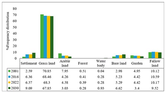
Figure 2.
The percentage of LULCC (2001–2030).
3.2. Validation of the Model
The agreement of the two categorical maps was measured by using a validation module. In order to assess accuracy, the validation of the model is necessary. Validation is essential because it allows for determining the quality of the predicted land cover/land use map when compared to the actual map. The coefficient of kappa and overall accuracy were 0.75 and 82%, respectively. A comparison was made between the actual and simulated land cover/land use map of 2022 in order to validate the predicted map (Table 4).
Table 4.
LULC change prediction validation based on the actual and projected 2022 LULC.
According to Figure 3, most of the area is covered by Grass land, which is concentrated in the north and southwest, followed by Arable land in second place, with approximately 10%. The highest growth in settlement areas is related to cities IV, V, II, and VI, respectively, and this trend continues in the next 8 years for cities II and VI.
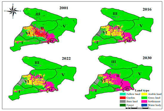
Figure 3.
Land use/Land cover changes (2001–2030).
3.3. Assessment of Biological Capacity in Productive Ecosystems
Biological capacity and the production coefficient were calculated for four productive ecosystems (desalinated water and brine resources, forest, grass lands, and agricultural lands) (Table 5). Water resources are the most productive natural resources of the country, and the production of desalinated water and petroleum resources plays a significant role. The biological capacity of the grass lands was calculated based on two parameters: (1) the mine and (2) the part of the petroleum production resources that are located in the grass lands. The biological capacity of the forests is affected by water, oxygen, wood production, and carbon sequestration.
Table 5.
Biological capacity of four productive ecosystems.
3.4. Ecological Footprint of Industries and Mines
- (A)
- Resource Consumption
The production capacity for industries was estimated at 76 × 106 tons. However, about 50% of that amount is currently exploited. So, the actual production capacity is 38 × tons. The different industries consume approximately 16.5 × 10⁶ tons of raw materials for this amount of production. This calculation includes industries that directly consume natural raw materials (petroleum, soil, minerals, agricultural products, wood, water, and natural fishery products). Moreover, the amount of raw materials that were extracted from mines is equal to 6.15 × 10⁶ tons. Then, the industrial units, which are used for the raw materials, were separated and coded in ArcGIS based on provincial and extra-provincial productive ecosystems (code 1 = forest, 2 = water resources, 3 = crop lands, 4 = grass lands). According to Table 6, the total amount of ecological footprint materials used in the province’s industries equals 1,543,260 hec.
Table 6.
The ecological footprint of raw resource consumption in different industries.
The raw materials used in mines in the study area were allocated to grass lands (6100 × 103 tons). The total amount of raw material ecological footprint in the mines equals 26.23 × 10³ hec.
- (B)
- Waste
The average productivity of the industries and mines is about 98% and 94%, respectively. Additionally, 20% of the country’s waste is subject to recycling and waste management. So, the amount of waste equals 2% and 6% of the consumed raw material from the industries and mines (1,465,527 tons). The ecological footprint of waste for the industries and mines equals 25,377 hec.
- (C)
- Energy
The ecological footprint of energy consumption in the industries and mines was calculated for different types of energy by considering the share of the productive ecosystems in producing energy. The ecological footprint of energy consumption was equal to 687.9 hec (Table 7).
Table 7.
The ecological footprint of energy consumption.
- (D)
- Pollution
The amount of pollutant emission from fuel consumption was calculated based on the emission coefficient [71]. Therefore, the amount of energy consumption was calculated, and the amount of energy production was converted based on BTU. The role of productive ecosystems in up-taking pollutants can be calculated according to their carbon sequestration capacity. Therefore, the share of forests, crop lands, grass lands, and water resources were 54%, 36%, 8%, and 2%, respectively. Additionally, for the eqf, Yf, and Y coefficients, their weighted averages were used, which were 25, 1.02, and 1.89, respectively. The ecological footprint of pollutant emissions was equal to 770,654 hec (Table 8).
Table 8.
The ecological footprint of pollutant emissions.
- (E)
- Water
The water footprint is an indicator showing the volume of water used directly or indirectly to produce goods or provide any services. It includes the sum of water consumed during the production chain processes of a product. Additionally, the amount of this index on an individual or social scale is equal to the total amount of water that a person consumes directly or indirectly and through various uses. It should be noted that in the first case, this index is expressed and presented as m2 per unit of the products, and in the second case, as m2 per year per individual or community. Indirect water consumption includes the volume of water that is used to produce a product or provide services for the benefit of an individual or a community. The water footprint calculation is divided into two parts: water consumption and wastewater generation (Table 9).
Table 9.
The ecological footprint of water consumption and wastewater generation.
Ecological Footprint of Agricultural, Service, and Household Consumption
The calculation of the ecological footprint of the agriculture, service, and household sectors was carried out using a similar approach to the industries and mines. However, some considerations were applied. All the data are available in detail upon request from the corresponding author.
- -
- In the agricultural sector, the EF calculation for resource consumption and waste emissions is a function of the cultivated land. A conversion matrix was used to convert resource consumption and waste emissions into the corresponding land areas [72,73,74]. Resource consumption in this sector is divided into pesticides and seeds [75,76]. According to [61,77], 25% of agricultural products are converted into waste;
- -
- In the household sector, the EF calculation for resource, energy, and water consumption, as well as waste, pollution, and wastewater emissions, is a function of population. Each citizen in the study area produces 700 g of waste per day, about 100 g more than average in Iran. However, 20% of the amount is recycled;
- -
- In the service sector, the EF calculation includes transportation and tourism [78,79]. Resources consumption and waste emissions in the transportation sector, as well as energy consumption, and pollutant emissions in the tourism sector, were not significant, so these indicators were not considered in this sector. The tourist population was equal to 2,261,896 persons per night, each producing approximately 900 g of waste in the study area.
3.5. Estimating the Ecological Carrying Capacity, Biological Capacity, and Ecological Footprint
According to Figure 4, biological capacity has decreased moderately since 1988, while ecological footprint has increased and reached a peak of 3630.82 × 103 hec in 2022. The ecological deficit in the study area equals −2562.62 × 103 hec in 2022. This means that the development trend caused the study area to be −2562.62 × 103 hec in debt to the country in 2022. The trend of changing indicators shows that the biological deficit of the study area has been decreasing, and the principle of resource capital has been used regardless of its ability to recover. According to the development process, the study area’s biological reserves were completed in 1992.
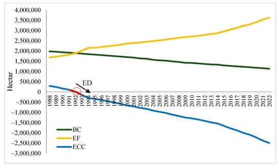
Figure 4.
Estimating biological capacity, ecological footprint, ecological deficit, and ecological carrying capacity (1988–2022).
3.6. Scenarios
The process of ecological footprint calculation illustrates which indicators have a significant effect on it. The results show that the highest amount of ecological footprint is allocated to (a): the ecological footprint of resource consumption in industries and mines, (b): the ecological footprint of water consumption in agriculture and household consumption, (c): the ecological footprint of pollutant emissions in the industries and mines and household consumption (Table 10).
Table 10.
The analysis of ecological footprint in different sectors and six subjects.
In the ideal scenario, according to Alborz’s development policies, the maximum changes in the EF in different sectors were considered. These changes include the following:
- (a)
- 20% reduction in annual pollutants emission;
- (b)
- 85% recycling in waste;
- (c)
- 22% reduction in water consumption;
- (d)
- 30% reduction in agricultural water consumption;
- (e)
- 80% recycling of agricultural wastewater;
- (f)
- 25% reduction in raw material consumption in the food industry.
According to Table 11, if the maximum changes were considered in the EF, the ecological deficit would increase from −2557.43 to −1652.55 × 103 hec. This means the study area can rehabilitate 904,881 hec compared with the current ecological deficit. So, Alborz Province will lose its ability to rehabilitate when it reaches −3462.31 × 103 hec in about 2030 (Figure 4).
Table 11.
Ecological footprint changes based on the measures.
3.6.1. Continuing Current Status
Based on Figure 5, if the current status continues, the study area will face a lack of ecological reconstruction ability by 2030, when the ED reaches −3497.36 × 103 hec.
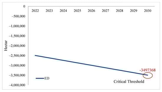
Figure 5.
Estimating the ecological deficit (2022–2030).
3.6.2. Sustainable Scenario
In order to achieve ecological balance in Alborz, short-, medium-, and long-term scenarios are proposed as follows: (a) preventing the ED from reaching the critical threshold in 2030; (b) maintaining the ecological deficit at the same level until 2043, and (c) bringing Alborz to ecological balance (bringing the ecological deficit to zero) by 2072.
Short-Term Scenario: Preventing the ED from Reaching the Critical Threshold of Ecological Deficit by 2030
By 2030, the ecological deficit of Alborz Province should have increased by about 904.88 × 10³ hec with the following measures: reducing pollutant emissions in all sectors by 2.5% per year; increasing waste recycling in the agricultural and service sectors by 10% per year; reducing agricultural water consumption by 3.5% per year; increasing agricultural wastewater recycling by 10% per year; reducing the consumption of raw materials in the food industries by 3% per year.
Mid-Term Scenario: Maintaining the ED at the Same Level until 2043
The ecological deficit will fall out of the critical point if short-term ecological deficit policies are implemented in 2030. However, the increase in the ecological footprint and ecological deficit, and consequently, the decrease in the biological capacity, will continue. The continuation of this situation will cause a crisis to recur and reach the ecological deficit critical point again in the following years. So, measures should be taken to prevent the ecological deficit from exceeding the critical threshold until 2043. These include but are not limited to a reduction in pollutant emissions in all sectors by 5% per year; increasing waste recycling in agriculture and services by 15% per year; reducing the water consumption of all sectors by 3% per year; reducing agricultural water consumption by 5% per year; increasing agricultural wastewater recycling by 15% per year from 2030 and 20% per year from 2036; continuing to reduce the consumption of raw materials in the food industries by 5% per year.
Long-Term Scenario: Returning the ED to 0
By implementing mid-term measures, the study area’s reconstruction ability will be maintained until 2043. However, if the ecological deficit continues in the long run, the study area will deplete the ecological reserves. Therefore, measures should be taken to return the region to the point of using products instead of reserves (ecological deficit = 0); this is important in long-term planning until the horizon of 2072. The realization of this scenario is possible by completing and strengthening the mid-term scenario preparations as follows: reducing pollutants emission in all sectors by 10% per year from 2045 and 15% from 2061; increasing waste recycling in agriculture and services by 20% per year; reducing water consumption in all sectors 5% per year; reducing agricultural water consumption 10% per year; increasing agricultural wastewater recycling by 20% per year from 2061; reducing energy consumption by 5% per year. Moreover, preventing the reduction in grass lands and agricultural lands in favor of increasing settlement areas by leading the population to other potential areas. Figure 6 shows that the ecological deficit will reach 0 in 2072.
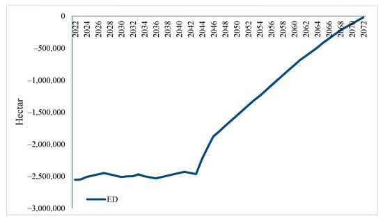
Figure 6.
Predicting the ecological deficit if scenarios are applied.
4. Discussion
Human activity must consider the ecological limitations of planet Earth in order to be sustainable. Environmental carrying capacity evaluates ecological limits and quantifies human impact, as well as the level that can be tolerated by the environment. Its usage reduces the risk of the unsustainable production and consumption of mankind. Ecological footprint and biological capacity are indicators that can be used to assess the environmental carrying capacity of a study area. Therefore, decision-makers can use these indicators in land-use planning and extract operational plans for sustainable development [80]. This study attempted to estimate ecological sustainability and achieve the desired balance between urban-area development and environmental conservation.
The study area is considered one of the most important areas for agriculture and livestock in Iran due to its moderate climate and enriched grass lands. Moreover, the population has been increasing in the study area because of its location close to the capital (Tehran), and the industries it provides, which provide jobs. The results demonstrated that the settlement areas increased from 2.5% in 2001 to 6.5% in 2022, and this figure will reach 9% in the following 8 years. Almost 70% of the studied area is covered by grass lands, which decreased by 3%. The area of arable lands and forests reduced by 4% and 0.3%, respectively, over 21 years.
The results show that the ecological footprint has already exceeded the biological capacity since 1992, and the study area is in an ecological deficit. However, on the one hand, the study area will lose its ecological regeneration capacity under the continuation of LULCC and the reduction in the area of productive ecosystems, such as grass lands, water resources, and forests, in favor of settlement areas and on the other, it will see increasing pressure on natural reserves, especially in resource consumption and pollution generation via industry, the water consumption in agriculture, and the water consumption and pollution generated by household consumption. This means that the use of reserves has outstripped the natural regenerative rate of the resources, and by continuing the current trend, a worse environmental crisis will occur.
5. Conclusions
In the present study, the environmental carrying capacity model (i.e., ecological footprint and biological capacity) is selected to assess ecological sustainability and achieve the desired balance. The environmental carrying capacity is a tool for better sustainable spatial management [81], and its implementation is essential for managing resource consumption properly and environmental planning in Iran [82].
Our study suggests that the agriculture sector stands first in terms of increasing ecological footprint, followed by the industry sector in second place. The ecological footprint of the sectors has risen through the consumption of resources and water. Moreover, the country’s resources and biological capacity are limited and specific, which means the demands cannot exceed the biological capacity. By exerting more pressure on resources, the possibility of reconstruction has been eliminated, and human life and the environment will be in danger. The results show that the formulation of short-term operational plans, like reducing agricultural water consumption [83], recycling waste and wastewater, and reducing emissions, can have a positive effect on reducing the footprint of the province.
In addition, we have only focused on the dynamic changes in the ECC in this paper; the spatial changes in the region’s ECC have not been considered. Future studies should take into account the spatial changes in the region’s ecological footprint and biological capacity. Finally, the outcomes of this study present some valuable information that can guide policymakers and planners in deciding on sustainable land use.
Author Contributions
Writing—original draft, S.P., M.H., Z.E. and H.H.; Writing—review & editing, K.E.L., S.P. and Z.E.; Funding acquisition, K.E.L. and C.T.G. All authors have read and agreed to the published version of the manuscript.
Funding
This research was funded by the University of Tehran and the University Kebangsaan Malaysia through PP-LESTARI-2023 and XX-2022-003.
Institutional Review Board Statement
Not applicable.
Informed Consent Statement
Not applicable.
Data Availability Statement
The data presented in this study are available on request from the corresponding author.
Acknowledgments
We acknowledge the University of Tehran, the University of Kharazmi, and the Universiti Kebangsaan Malaysia for their provision of resources and collaborative efforts.
Conflicts of Interest
The authors declare no conflict of interest.
References
- Liu, Z.; Ding, M.; He, C.; Li, J.; Wu, J. The impairment of environmental sustainability due to rapid urbanization in the dryland region of northern China. Landsc. Urban Plan. 2019, 187, 165–180. [Google Scholar] [CrossRef]
- Golia, E.E.; Papadimou, S.G.; Cavalaris, C.; Tsiropoulos, N.G. Level of Contamination Assessment of Potentially Toxic Elements in the Urban Soils of Volos City (Central Greece). Sustainability 2021, 13, 2029. [Google Scholar] [CrossRef]
- Christoforidis, A.; Stamatis, N. Heavy metal contamination in street dust and roadside soil along the major national road in Kavala’s region, Greece. Geoderma 2009, 151, 257–263. [Google Scholar] [CrossRef]
- Ahmed, Z.; Asghar, M.M.; Malik, M.N.; Nawaz, K. Moving towards a sustainable environment: The dynamic linkage between natural resources, human capital, urbanization, economic growth, and ecological footprint in China. Resour. Policy 2020, 67, 101677. [Google Scholar] [CrossRef]
- Burger, J.R.; Allen, C.D.; Brown, J.H.; Burnside, W.R.; Davidson, A.D.; Fristoe, T.S.; Okie, J.G. The macroecology of sustainability. PLoS Biol. 2012, 10, 1001345. [Google Scholar] [CrossRef]
- Imhoff, M.L.; Bounoua, L.; Ricketts, T.; Loucks, C.; Harriss, R.; Lawrence, W.T. Global patterns in human consumption of net primary production. Nature 2004, 429, 870–873. [Google Scholar] [CrossRef] [PubMed]
- Rees, W.E. Ecological footprints and appropriated carrying capacity: What urban economics leaves out. Urbanization 2017, 2, 66–77. [Google Scholar] [CrossRef]
- Wang, Z.; Gao, Y.; Wang, X.; Lin, Q.; Li, L. A new approach to land use optimization and simulation considering urban development sustainability: A case study of Bortala, China. Sustain. Cities Soc. 2022, 87, 104135. [Google Scholar] [CrossRef]
- Genta, C.; Sanyé-Mengual, E.; Sala, S.; Lombardi, P. The Consumption Footprint as possible indicator for environmental impact evaluation at city level. Case Study Turin (Italy). Sustain. Cities Soc. 2022, 79, 103679. [Google Scholar] [CrossRef]
- He, Y.; Xie, H. Exploring the spatiotemporal changes of ecological carrying capacity for regional sustainable development based on GIS: A case study of Nanchang City. Technol. Forecast. Soc. Chang. 2019, 148, 119720. [Google Scholar] [CrossRef]
- Van den Bergh, J.C.; Grazi, F. Ecological footprint policy? Land use as an environmental indicator. J. Ind. Ecol. 2014, 18, 10–19. [Google Scholar] [CrossRef]
- Borucke, M.; Moore, D.; Cranston, G.; Gracey, K.; Iha, K.; Larson, J.; Lazarus, E.; Morales, J.C.; Wackernagel, M.; Galli, A. Accounting for demand and supply of the biosphere’s regenerative capacity: The National Footprint Accounts’ underlying methodology and framework. Ecol. Indic. 2013, 24, 518–533. [Google Scholar] [CrossRef]
- Bruckner, M.; Fischer, G.; Tramberend, S.; Giljum, S. Measuring telecouplings in the global land system: A review and comparative evaluation of land footprint accounting methods. Ecol. Econ. 2015, 114, 11–21. [Google Scholar] [CrossRef]
- Charfeddine, L. The impact of energy consumption and economic development on ecological footprint and CO2 emissions: Evidence from a Markov switching equilibrium correction model. Energy Econ. 2017, 65, 355–374. [Google Scholar] [CrossRef]
- Moran, D.D.; Wackernagel, M.; Kitzes, J.A.; Goldfinger, S.H.; Boutaud, A. Measuring sustainable development—Nation by nation. Ecol. Econ. 2008, 64, 470–474. [Google Scholar] [CrossRef]
- Wackernagel, M.; Monfreda, C.; Moran, D.; Wermer, P.; Goldfinger, S.; Deumling, D.; Murray, M. National Footprint and Biocapacity Accounts: The Underlying Calculation Method; Global Footprint Network: Oakland, CA, USA, 2005; pp. 4–28. [Google Scholar]
- Galli, A.; Iha, K.; Pires, S.M.; Mancini, M.S.; Alves, A.; Zokai, G.; Lin, D.; Murthy, A.; Wackernagel, M. Assessing the ecological footprint and biocapacity of Portuguese cities: Critical results for environmental awareness and local management. Cities 2020, 96, 102442. [Google Scholar] [CrossRef]
- Świąder, M.; Szewrański, S.; Kazak, J.K.; Van Hoof, J.; Lin, D.; Wackernagel, M.; Alves, A. Application of ecological footprint accounting as a part of an integrated assessment of environmental carrying capacity: A case study of the footprint of food of a large city. Resources 2018, 7, 52. [Google Scholar] [CrossRef]
- Tan, S.; Liu, Q.; Han, S. Spatial-temporal evolution of coupling relationship between land development intensity and resources environment carrying capacity in China. J. Environ. Manag. 2022, 301, 113778. [Google Scholar] [CrossRef]
- Wang, X. Managing land carrying capacity: Key to achieving sustainable production systems for food security. Land 2022, 11, 484. [Google Scholar] [CrossRef]
- Zhang, Z.; Hu, B.; Qiu, H. Comprehensive evaluation of resource and environmental carrying capacity based on SDGs perspective and Three-dimensional Balance Model. Ecol. Indic. 2022, 138, 108788. [Google Scholar] [CrossRef]
- Arto, I.; Rueda-Cantuche, J.M.; Peters, G.P. Comparing the GTAP-MRIO and WIOD databases for carbon footprint analysis. Econ. Syst. Res. 2014, 26, 327–353. [Google Scholar] [CrossRef]
- Hoekstra, A.Y.; Wiedmann, T.O. Humanity’s unsustainable environmental footprint. Science 2014, 344, 1114–1117. [Google Scholar] [CrossRef] [PubMed]
- O’Neill, D.W.; Fanning, A.L.; Lamb, W.F.; Steinberger, J.K. A good life for all within planetary boundaries. Nat. Sustain. 2018, 1, 88–95. [Google Scholar] [CrossRef]
- Tsuchiya, K.; Iha, K.; Murthy, A.; Lin, D.; Altiok, S.; Rupprecht, C.D.; Kiyono, H.; McGreevy, S.R. Decentralization & local food: Japan’s regional Ecological Footprints indicate localized sustainability strategies. J. Clean. Prod. 2021, 292, 126043. [Google Scholar] [CrossRef]
- Mohapatra, S.; Joseph, G.; Ratha, D. Remittances and natural disasters: Ex-post response and contribution to ex-ante preparedness. Environ. Dev. Sustain. 2012, 14, 365–387. [Google Scholar] [CrossRef]
- Ewing, B.R.; Hawkins, T.R.; Wiedmann, T.O.; Galli, A.; Ercin, A.E.; Weinzettel, J.; Steen-Olsen, K. Integrating ecological and water footprint accounting in a multi-regional input–output framework. Ecol. Indic. 2012, 23, 1–8. [Google Scholar] [CrossRef]
- Chambers, J.C.; Bradley, B.A.; Brown, C.S.; D’Antonio, C.; Germino, M.J.; Grace, J.B.; Hardegree, S.P.; Miller, R.F.; Pyke, D.A. Resilience to stress and disturbance, and resistance to Bromus tectorum L. invasion in cold desert shrublands of western North America. Ecosystems 2014, 17, 360–375. [Google Scholar] [CrossRef]
- Mancini, M.S.; Galli, A.; Coscieme, L.; Niccolucci, V.; Lin, D.; Pulselli, F.M.; Bastianoni, S.; Marchettini, N. Exploring ecosystem services assessment through Ecological Footprint accounting. Ecosyst. Serv. 2018, 30, 228–235. [Google Scholar] [CrossRef]
- Lin, D.; Hanscom, L.; Murthy, A.; Galli, A.; Evans, M.; Neill, E.; Mancini, M.S.; Martindill, J.; Medouar, F.Z.; Huang, S.; et al. Ecological footprint accounting for countries: Updates and results of the National Footprint Accounts, 2012–2018. Resources 2018, 7, 58. [Google Scholar] [CrossRef]
- Özbaş, E.E.; Hunce, S.Y.; Özcan, H.K.; Öngen, A. Ecological Footprint Calculation. Recycl. Reuse Approaches Better Sustain. 2019, 8, 179–186. [Google Scholar] [CrossRef]
- Sylla, M. Mapping and assessment of the potential to supply selected ecosystem services at a sub-regional scale. Ex. Wroc. Its Surround. Munic. Ekon. I Środowisko-Econ. Environ. 2016, 59, 12. [Google Scholar]
- Budihardjo, S.; Hadi, S.P.; Sutikno, S.; Purwanto, P. The ecological footprint analysis for assessing carrying capacity of industrial zone in Semarang. J. Hum. Resour. Sustain. Stud. 2013, 1, 33057. [Google Scholar] [CrossRef]
- Galli, A.; Halle, M.; Grunewald, N. Physical limits to resource access and utilization and their economic implications in Mediterranean economies. Environ. Sci. Policy 2015, 51, 125–136. [Google Scholar] [CrossRef]
- Long, X.; Yu, H.; Sun, M.; Wang, X.C.; Klemeš, J.J.; Xie, W.; Wang, C.; Li, W.; Wang, Y. Sustainability evaluation based on the Three-dimensional Ecological Footprint and Human Development Index: A case study on the four island regions in China. J. Environ. Manag. 2020, 265, 110509. [Google Scholar] [CrossRef]
- Wu, F.; Yang, X.; Shen, Z.; Bian, D.; Babuna, P. Exploring sustainability and decoupling effects of natural capital utilization in China: Evidence from a provincial three-dimensional ecological footprint. J. Clean. Prod. 2021, 295, 126486. [Google Scholar] [CrossRef]
- Al-hadithy, A. Urban Planning Ecological footprint and its impact on city sustainability Ecological footprint and its impact on city sustainability. Urban Plan. 2022, 6, 1–23. [Google Scholar] [CrossRef]
- Xie, B.; Zhang, X.; Lu, J.; Liu, F.; Fan, Y. Research on ecological evaluation of Shanghai port logistics based on emergy ecological footprint models. Ecol. Indic. 2022, 139, 108916. [Google Scholar] [CrossRef]
- Clark, T.P.; Longo, S.B. Examining the effect of economic development, region, and time period on the fisheries footprints of nations (1961–2010). Int. J. Comp. Sociol. 2019, 60, 225–248. [Google Scholar] [CrossRef]
- Kong, F.; Cui, W.; Xi, H. Spatial–temporal variation, decoupling effects and prediction of marine fishery based on modified ecological footprint model: Case study of 11 coastal provinces in China. Ecol. Indic. 2021, 132, 108271. [Google Scholar] [CrossRef]
- Akrour, S.; Grimes, S. Is the Ecological Footprint Enough Science for Algerian Fisheries Management? Sustainability 2022, 14, 1418. [Google Scholar] [CrossRef]
- Ahmed, Z.; Wang, Z. Investigating the impact of human capital on the ecological footprint in India: An empirical analysis. Environ. Sci. Pollut. Res. 2019, 26, 26782–26796. [Google Scholar] [CrossRef] [PubMed]
- Destek, M.A.; Ulucak, R.; Dogan, E. Analyzing the environmental Kuznets curve for the EU countries: The role of ecological footprint. Environ. Sci. Pollut. Res. 2018, 25, 29387–29396. [Google Scholar] [CrossRef]
- Shakeel, M. Analyses of energy-GDP-export nexus: The way-forward. Energy 2021, 216, 119280. [Google Scholar] [CrossRef]
- Chezgi, J.; Pourghasemi, H.R.; Naghibi, S.A.; Moradi, H.R.; Kheirkhah Zarkesh, M. Assessment of a spatial multi-criteria evaluation to site selection underground dams in the Alborz Province, Iran. Geocarto Int. 2016, 31, 628–646. [Google Scholar] [CrossRef]
- Arbabi, Z.; Yeganegi, K.; Obaid, A.J. Application of neural networks in evaluation of key factors of knowledge management system, Case Study: Iranian Companies Based in Alborz Province. J. Phys. 2020, 1530, 012111. [Google Scholar] [CrossRef]
- Nath, B.; Wang, Z.; Ge, Y.; Islam, K.P.; Singh, R.; Niu, Z. Land use and land cover change modeling and future potential landscape risk assessment using Markov-CA model and analytical hierarchy process. ISPRS Int. J. Geo-Inf. 2020, 9, 134. [Google Scholar] [CrossRef]
- Nguyen, H.T.T.; Pham, T.A.; Doan, M.T.; Tran, P.T.X. Land use/land cover change prediction using multi-temporal satellite imagery and multi-layer perceptron markov model. Int. Arch. Photogramm. Remote Sens. Spat. Inf. Sci. ISPRS Arch. 2020, 54, 99–105. [Google Scholar] [CrossRef]
- Nguyen, T.T.H.; Ngo, T.T.P. Land use/land cover change prediction in Dak Nong Province based on remote sensing and Markov Chain Model and Cellular Automata. J. Vietnam. Environ. 2018, 9, 132–140. [Google Scholar] [CrossRef]
- Hamad, R.; Balzter, H.; Kolo, K. Predicting land use/land cover changes using a CA-Markov model under two different scenarios. Sustainability 2018, 10, 3421. [Google Scholar] [CrossRef]
- Eastman, J.R. TerrSet Geospatial Monitoring and Modeling System–Manual; Clark University: Worcester, MA, USA, 2016; p. 395. [Google Scholar]
- Abdulrahman, A.I.; Ameen, S.A. Predicting Land use and land cover spatiotemporal changes utilizing CA-Markov model in Duhok district between 1999 and 2033. Acad. J. Nawroz Univ. 2020, 9, 71–80. [Google Scholar] [CrossRef]
- Schaefer, F.; Luksch, U.; Steinbach, N.; Cabeça, J.; Hanauer, J. Ecological Footprint and Biocapacity: The World’s Ability to Regenerate Resources and Absorb Waste in a Limited Time Period. Office for Official Publications of the European Communities, Luxembourg. 2006. Available online: http://ec.europa.eu/eurostat/documents/3888793/5835641/KSAU-06-001-EN.PDF (accessed on 28 December 2016).
- Neagu, O. Economic Complexity and Ecological Footprint: Evidence from the Most Complex Economies in the World. Sustainability 2020, 12, 9031. [Google Scholar] [CrossRef]
- Wiedmann, T.; Barrett, J. A Review of the Ecological Footprint Indicator—Perceptions and Methods. Sustainability 2010, 2, 1645–1693. [Google Scholar] [CrossRef]
- Hausmann, R.; Hidalgo, C.A.; Bustos, S.; Coscia, M.; Simoes, A.; Yildirim, M.A. The Atlas of Economic Complexity: Mapping Paths to Prosperity; MIT Press: Cambridge, MA, USA, 2014. [Google Scholar]
- Vaisi, S.; Alizadeh, H.; Lotfi, W.; Mohammadi, S. Developing the Ecological Footprint Assessment for a University Campus, the Component-Based Method. Sustainability 2021, 13, 9928. [Google Scholar] [CrossRef]
- Kitzes, J.; Galli, A.; Bagliani, M.; Barrett, J.; Dige, G.; Ede, S.; Erb, K.; Giljum, S.; Haberl, H.; Hails, C.; et al. A research agenda for improving national Ecological Footprint accounts. Ecol. Econ. 2009, 68, 1991–2007. [Google Scholar] [CrossRef]
- Costa, I.; Martins, F.G.; Alves, I. Ecological footprint as a sustainability indicator to analyze energy consumption in a Portuguese textile facility. Int. J. Energy Environ. Eng. 2019, 10, 523–528. [Google Scholar] [CrossRef]
- Costanza, R. The dynamics of the ecological footprint concept. Ecol. Econ. 2000, 32, 341–345. [Google Scholar] [CrossRef]
- DeLurgio, S.A. Forecasting Principles and Applications; McGraw-Hill/Irwin: Philadelphia, PA, USA, 1998. [Google Scholar]
- Box, G. Box and Jenkins: Time Series Analysis, Forecasting and Control. In A Very British Affair. Palgrave Advanced Texts in Econometrics; Palgrave Macmillan: London, UK, 2013. [Google Scholar] [CrossRef]
- Agriculture-Jahad-Alborz, 2015–2016. Available online: https://alborz.maj.ir/page-alborzmain/FA/98/form/pId15634 (accessed on 12 November 2022).
- Alborz Environmental Yearbook. 2018. Available online: https://alborz.mporg.ir/Portal/View/Page.aspx?PageId=d5bb27ec-5669-4e2c-9b82-593becc970e4 (accessed on 1 November 2022).
- Energy Yearbook. Production, Trade and Supply of Natural Gas; Statistical Centre of Iran: Tehran, Iran, 2016; Available online: https://irandataportal.syr.edu/ (accessed on 20 November 2022).
- IMTY. Industry, Mine, and Trade Yearbook, 2006–2022. Available online: https://en.mimt.gov.ir/ (accessed on 5 December 2022).
- ISY. Iran Statistical Yearbooks, 2009–2022. Available online: https://www.amar.org.ir/english (accessed on 17 December 2022).
- SYE. Statistical Yearbook Energy, 1990–2021. Available online: https://pep.moe.gov.ir (accessed on 3 October 2022).
- SYF. Statistical Yearbook of Fisheries, 1999–2021. Available online: http://www.fisheries.ir/site/News_view.aspx?id=113032&tbl=N (accessed on 20 December 2022).
- Miao, Y.; Blunsom, P. Language as a latent variable: Discrete generative models for sentence compression. arXiv 2016, arXiv:1609.07317. [Google Scholar] [CrossRef]
- IPCC. Inter-Governmental Panel on Climate Change—Organization of IPCC. 2014. Available online: http://www.ipcc.ch/organization/organization.shtml#.UvnDl_mSzCs (accessed on 11 February 2014).
- Liang, H.; Zou, J.; Li, Z.; Khan, M.J.; Lu, Y. Dynamic evaluation of drilling leakage risk based on fuzzy theory and PSO-SVR algorithm. Future Gener. Comput. Syst. 2019, 95, 454–466. [Google Scholar] [CrossRef]
- Liang, H.; Zou, J.; Zuo, K.; Khan, M.J. An improved genetic algorithm optimization fuzzy controller applied to the wellhead back pressure control system. Mech. Syst. Signal Process. 2020, 142, 106708. [Google Scholar] [CrossRef]
- Zhang, Y.; Zhu, R.; Chen, Z.; Gao, J.; Xia, D. Evaluating and selecting features via information theoretic lower bounds of feature inner correlations for high-dimensional data. Eur. J. Oper. Res. 2020, 290, 235–247. [Google Scholar] [CrossRef]
- Passeri, N.; Borucke, M.; Blasi, E.; Franco, S.; Lazarus, E. The Influence of Farming Technique on Cropland: A New Approach for the Ecological Footprint. Ecol. Indic. 2013, 29, 1–5. [Google Scholar] [CrossRef]
- Kool, A.; Marinussen, M.; Blonk, H. LCI Data for the Calculation Tool Feedprint for Greenhouse Gas Emissions of Feed Production and Utilization. GHG Emissions of N, P and K Fertiliser Production; Blonk Consultants: Gouda, The Netherlands, 2012. [Google Scholar]
- Khosravani, F.; PezeshkiRad, G.; Farhadian, H. Investigating the status of agricultural waste and waste and providing management solutions in order to achieve the goals of sustainable development. Promot. Sci. 2013, 3, 95–112. [Google Scholar]
- Aboelnaga, S.; Tóth, T.; Neszmélyi, G. Calculations on ecological footprint as a tool for land use planning and development on v4 countries. Cent. Eur. J. Reg. Dev. Tour. 2021, 13, 24–39. [Google Scholar] [CrossRef]
- Wiedmann, T.; Minx, J.; Barrett, J.; Wackernagel, M. Allocating ecological footprints to final consumption categories with input–output analysis. Ecol. Econ. 2006, 56, 28–48. [Google Scholar] [CrossRef]
- Clift, R.; Sim, S.; King, H.; Chenoweth, J.L.; Christie, I.; Clavreul, J.; Mueller, C.; Posthuma, L.; Boulay, A.-M.; Chaplin-Kramer, R.; et al. The Challenges of Applying Planetary Boundaries as a Basis for Strategic Decision-Making in Companies with Global Supply Chains. Sustainability 2017, 9, 279. [Google Scholar] [CrossRef]
- McPhearson, T.; Haase, D.; Kabisch, N.; Gren, Å. Advancing understanding of the complex nature of urban systems. Ecol. Indic. 2016, 70, 566–573. [Google Scholar] [CrossRef]
- Fatemi, M.; Rezaei-Moghaddam, K.; Karami, E.; Hayati, D.; Wackernagel, M. An integrated approach of Ecological Footprint (EF) and Analytical Hierarchy Process (AHP) in human ecology: A base for planning toward sustainability. PLoS ONE 2021, 16, 0250167. [Google Scholar] [CrossRef]
- Zeshan, M.; Shakeel, M. Adaptations and mitigation policies to climate change: A dynamic CGE-WE model. Singap. Econ. Rev. 2020, 1, 1–25. [Google Scholar] [CrossRef]
Disclaimer/Publisher’s Note: The statements, opinions and data contained in all publications are solely those of the individual author(s) and contributor(s) and not of MDPI and/or the editor(s). MDPI and/or the editor(s) disclaim responsibility for any injury to people or property resulting from any ideas, methods, instructions or products referred to in the content. |
© 2023 by the authors. Licensee MDPI, Basel, Switzerland. This article is an open access article distributed under the terms and conditions of the Creative Commons Attribution (CC BY) license (https://creativecommons.org/licenses/by/4.0/).