An Energy Management Strategy for Fuel-Cell Hybrid Commercial Vehicles Based on Adaptive Model Prediction

Abstract

Fuel-cell hybrid electric vehicles have the advantages of zero pollution and high efficiency and are extensively applied in commerce. An energy management strategy (EMS) directly impacts the fuel consumption and performance. Moreover, model prediction control (MPC) is synchronous and has been a research hotspot of EMS in recent years. The existing MPC’s low-speed prediction accuracy, which results in considerable instability in EMS allocation, is solved by the proposed energy management strategy based on adaptive model prediction. Dynamic programming (DP) is used as the solver, improved condition recognition and a radial basis neural network (RBFNN) are used as the speed predictor, and hydrogen consumption and the state of charge (SOC) are used as the objective function. According to the simulation results, using a 5 s speed prediction improves the forecast accuracy by 9.75%, and compared with employing a rule-based energy management strategy, this strategy reduces hydrogen consumption and the power cell fluctuation frequency by 3.50%.

1. Introduction

Traditional vehicles consume fossil fuels. This exacerbates the energy crisis and leads to the greenhouse effect and environmental pollution [1]. Fuel-cell vehicles utilize fuel cells as their main power source, and producing zero pollution and improving their performance have become research focuses [2,3]. Proton-exchange membrane fuel cells (PEMFC) have a high power density and low operating temperature and are extensively utilized in vehicles [4]. They often need to be equipped with auxiliary power due to the shortcomings of fuel cells, e.g., their poor dynamic response, short lifespan, and inability to recover energy. Currently, traction batteries and supercapacitors are utilized as auxiliary sources.

Fuel-cell vehicles have three structures [5,6]: fuel cell and traction battery; fuel cell and supercapacitor; fuel cell, traction battery, and supercapacitor. The fuel cell and traction battery structure is currently ubiquitous due to the low capacity and high price of supercapacitors. An energy management strategy (EMS) is crucial to impact the power and costs of fuel-cell hybrid vehicles equipped with multiple energy sources [7]. Currently, EMSs have three categories [8]: rule-based strategies, optimization-based strategies, and learning-based strategies.

Rule-based strategies are widely employed by car manufacturers. Engineering experience is required to set the threshold values [9,10]. Wang et al. [11] predicted traction batteries’ and supercapacitors’ powers under known conditions and discussed different combined working modes and rules for the three power sources. They significantly decreased hydrogen consumption. Simple deterministic rule strategies do not result in greater fuel consumption savings. Wang et al. [12] combined condition recognition and fuzzy rules to establish fuzzy rules for the energy management of each condition. The center and width of the fuzzy-rule membership function were optimized utilizing a genetic algorithm. Since the threshold values for the rule-based strategies were primarily determined by expert experience and experts sense was the primary factor, optimal energy allocation could not be achieved [13].

With the rapid growth of chips in recent years, learning-based strategies and optimization- based strategies have received a lot of attention [14,15,16]. Li et al. [17] pre-initialized the Q meter with the correlation rule to accelerate the Q learning algorithm convergence rate. Moreover, the driving condition was modeled as a Markov process. Fuel-cell system (FCS) power disparities of adjacent processes were employed to evaluate the impact on FCS longevity, which extended the service life of FCS. Learning-based strategies require potent computing power. Consequently, excellent in-vehicle chips are indispensable [18,19]; however, they only currently exist in theoretical research. Optimization-based strategies [20] in which dynamic programming (DP) reaches a global optimal [21,22] are only used as a standard for other strategies since the global operating conditions need to be obtained before implementation. The equivalent consumption minimization strategy (ECMS) is an instantaneous optimization strategy that achieves sub-optimal results [23]. Zou et al. [24] utilized wavelet transformation to convert the required power into high and low frequencies. The high frequency was from supercapacitors and the low frequency was from fuel cells and traction batteries. Consequently, the state of charge (SOC) optimal curve was utilized to design the equivalent factors. The equivalent factors in the ECMS were set under fixed conditions. Therefore, their applicability was impoverished as a result of other conditions. The model predictive energy management strategy, which combines the benefits of global and instantaneous optimization, overcomes the disadvantage of global optimization not being able to obtain the global operating conditions. Moreover, it can deal with a wide range of limited issues and, thus, has received a lot of attention [25].

Model prediction control (MPC) is characterized by the ability to forecast future velocities over a short time horizon and the use of optimization algorithms as solvers to allocate energy flows in real time [26]. Zhou et al. [27] built an MPC energy management approach by employing a library of typical working situations, a Markov condition recognizer, and an Elman neural network as the speed predictor. Yan et al. [28] achieved real-time energy distribution by combining condition recognition, Markov velocity, and Pontryagin’s minimal principle (PMP) as an energy source distribution solver. Because vehicles have a time domain and locality, using driving cycle libraries as conditions for specific vehicle designs produces a poor match, and the small amount of data from standard driving cycle libraries train the network with poor accuracy [25,29]. Each strategy has its own characteristics, and Table 1 summarizes the advantages and disadvantages of each EMS.

Table 1. Summary and comparison of energy management strategies (EMSs).

EMS		Advantage	Disadvantage
Rule-based strategies		Small calculations, low requirements for in-vehicle chips, easy to design.	Dependence on expert experience, low fuel economy, very poor serviceability.
Optimization-based strategies	DP	Theoretical optimal economy;	Need to obtain full cycle conditions;
	ECMS	Real-time, no complete loop conditions required;	The equivalent factor is difficult to obtain;
	MPC	Excellent dynamic control performance, and robustness.	Low accuracy of velocity prediction, and poor adaptability to cycle conditions.
Learning-based strategies		No need for physical model, high flexibility, balance economy and real-time performance.	Difficult and time-consuming data mining, lack of hardware test.

Consequently, this work proposed an energy management strategy based on adaptive model prediction. This paper has five main contributions. First, considering the small amount of data in the standard driving cycle library of commercial vehicles, we proposed to use a global positioning system (GPS) to retrieve the historical long series speed of the designed vehicle, pre-process the data according to wavelet filtering and mean processing, and apply principal component analysis (PCA) and K-means to classify the working conditions, which can better approximate the real operating conditions of the vehicle. Secondly, the back propagation neural network (BPNN) recognizer was trained, and the recognition accuracy was higher compared with the traditional recognition algorithm. Third, the combination of BPNN and radial basis neural network (RBFNN) improved the speed prediction accuracy. Fourthly, hydrogen consumption and SOC were used as cost functions to reduce the hydrogen consumption and SOC frequency fluctuations. Finally, a simulation was used to validate the effectiveness of the proposed method.

The rest of the work is arranged as follows. Section 2 introduces the fuel-cell hybrid electric vehicle model. Section 3 covers condition data processing and classification. Section 4 develops a rule-based energy management strategy and an energy management strategy based on adaptive model prediction. Section 5 simulates and discusses the results. Conclusions are drawn in Section 6.

2. Modeling of Fuel-Cell Hybrid Electric Vehicle

In this work, we selected the fuel-cell hybrid commercial vehicle model, and Figure 1 represents the topological structure. PEMFC and the traction battery were used as the main source and auxiliary source, respectively. The traction battery recovers energy in braking energy restoration, and the DC/DC converter connects with the bus and stabilizes the PEMFC voltage.

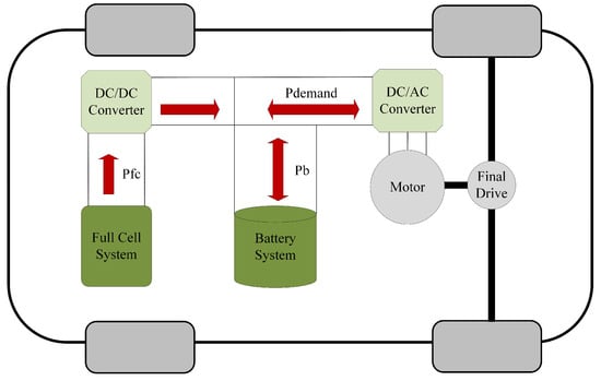
Figure 1. Structure of the fuel cell hybrid electric vehicle (FCHEV).

2.1. Vehicle Model

The vehicle longitudinal dynamics model was established and the lateral dynamics model disregarded. Driving resistance results from rolling, air, grade, and acceleration. The equation for tractive force $F_t$ is

$$F_t=mgfcos\left(\alpha \right)+1/2\rho C_{d}A{v}^2+mgsin\left(\alpha \right)+\delta mdv/dt$$

(1)

where m is vehicle mass; g is gravitational acceleration; f is the rolling resistance coefficient; $\alpha$ is the angle of the gradient; $\rho$ is air density; $C_d$ is the air resistance coefficient; A is the windward area; v is the vehicle speed; $\delta$ is the correction coefficient of rotating mass; $dv/dt$ is the accelerated speed. Table 2 shows the whole vehicle parameter table, and the total vehicle traction force can be calculated by plugging each parameter into Equation (1).

Table 2. Parameters of the full-cell vehicle.

Parameter	Value	Unit
Vehicle total mass, m	6000	kg
Wheel radius, r	0.375	m
Rolling resistance coefficient, f	0.012	-
Gravitational acceleration, g	9.8	m/s${}^2$
Air density, A	6.125	kg/m${}^3$
Aerodynamic drag coefficient, $C_d$	0.492	-
Final drive gear ratio, i	6.5071	-
Correction coefficient of rotating mass, $\delta$	1.05	-
Transmission efficiency, ${\eta }_{fd}$	95	%

Tractive force, speed, and vehicle rolling radius were calculated to acquire the wheel speed and torque:

$$w_w=v/r$$

(2)

$$T_w=r{F}_t$$

(3)

where $w_w$ is the wheel speed; $T_w$ is the wheel torque. The electrical-machinery rotational speed, torque, and power were calculated as follows:

$$w_m=w_{w}i$$

(4)

$$T_m=\left\{\begin{array}{ccc}{T}_w/\left({\eta }_{fd}i\right)& & T_w\ge 0\\ \left(T_w{\eta }_{fd}\right)/i& & T_w<0\end{array}\right.$$

(5)

$$P_m=\left\{\begin{array}{cc}\left(T_m{w}_m\right)/{\eta }_m& T_m\ge 0\\ T_m{w}_m{\eta }_m& T_m<0\end{array}\right.$$

(6)

where $w_m$ is the electrical-machinery rotational speed; $T_m$ is torque; $P_m$ is power; ${\eta }_m$ is efficiency. The electrical machinery does work on the vehicle with a positive torque; the electrical machinery charges the traction battery with a negative torque.

2.2. Fuel-Cell Model

PEMFCs with a high efficiency and fast response [30] are extensively applied in fuel-cell vehicles. A fuel-cell system includes an air compressor, a supply manifold, a return manifold, a humidifier, and a cooler. A complete fuel-cell system represents a real response better, and the model was simplified to achieve an instant response in the work. Fuel-cell power was determined by the maximum vehicle speed in the parametric design. Therefore, the work selected a fuel cell with a 60 KW rated output. Furthermore, the fuel-cell model was built considering the experiential model and the mathematical model [31,32].

$$V_{cell}=E_{nernst}-E_{act}-E_{ohimic}-E_{con}$$

(7)

where $V_{cell}$ is the output voltage of a single fuel cell; $E_{nernst}$ is the thermomechanical electromotive force; $E_{act}$ is activation polarization electromotive force; $E_{ohimic}$ is the ohmic polarization electromotive force; $E_{con}$ is the concentration polarization electromotive force. Demonstrates the ideal voltage without the dissipation of the thermomechanical electromotive force:

$$E_{nernst}=1.229-8.5 \times {10}^{-4} \times (T-T_0)+4.3085 \times {10}^{-5} \times T \times (0.5{ln}_{}{P}_{O2}+{ln}_{}{P}_{H2})$$

(8)

where T is thermomechanical temperature; $T_0$ is the reference temperature; $P_{O2}$ is the oxygen partial pressure; $P_{H2}$ is hydrogen partial pressure. The activation polarization electromotive force is calculated as follows:

$$E_{act}=V_0+V_a(1-e^{-c_{0}i})$$

(9)

$$V_0=0.279-8.5\times {10}^{-4}(T-T_0)+4.3085\times {10}^{-5}T\left[{ln}_{}\left(\frac{P_{ca}-P_{sat}}{1.101325}\right)+0.5{ln}_{}\frac{0.1173(P_{ca}-P_{sat})}{1.01325}\right]$$

(10)

$$V_a=(-1.618\times {10}^{-5}T+1.618\times {10}^{-2}){(\frac{P_{O2}}{0.1173}+P_{sat})}^2+(1.8\times {10}^{-4}T-0.166)(\frac{P_{O2}}{0.1173}+P_{sat})+(-5.8\times {10}^{-4}T+0.5736)$$

(11)

where $c_0$ is the coefficient (10); i is the current density; $P_{ca}$ is the cathode pressure; $P_{sat}$ is the steam saturation pressure. The ohmic polarization electromotive force is calculated by

$$E_{ohimic}=I{R}_{ohmic}=I(R_c+R_m)$$

(12)

$$R_m=\left({\rho }_{l}l\right)/S$$

(13)

$${\rho }_l=\frac{181.6[1+0.03i+0.062{(T/3.3)}^2{i}^{2.5}]}{(\lambda -0.634-3i)e^{\frac{4.18(T-303)}{T}}}$$

(14)

where I is the current; $R_{ohmic}$ is the internal resistance of a single fuel cell; $R_c$ is the proton transfer impedance; $R_m$ is the proton-exchange membrane equivalent impedance; ${\rho }_l$ is the proton-exchange membrane resistivity; l is the proton-exchange membrane thickness; S is the proton-exchange membrane effective contact area. Where l,S are calculated from Table 3. Equation (15) shows concentration polarization electromotive force.

$$E_{con}=\frac{-RT}{F}{ln}_{}(i/i_{max})$$

(15)

where R is the gas constant; F is the Faraday constant; $i_{max}$ is the maximum current density; where R, T, F are calculated from Table 3.

Table 3. Parameters of the proton-exchange membrane fuel cells (PEMFC).

Symbol	Parameter	Value
N	Number of cells in the stack	300
S	Full cell active area	280 cm${}^2$
l	Thickness of the membrane layer	50 $\mathsf{\mu }$m
R	Universal gas constant	8.314 J/(mol·k)
F	Faraday’s constant	96,485.34 C/mol
T	Fuel-cell temperature	353 K

The fuel-cell output power and hydrogen consumption rate were obtained using Equations (7)–(15):

$$P_{fcout}=N{V}_{cell}I$$

(16)

$${\dot{m}}_{H2}=\left(N{M}_{H2}\right)/nFI$$

(17)

where $P_{fcout}$ is fuel-cell system output power; N is the number of fuel cells; ${\dot{m}}_{H2}$ is the hydrogen consumption rate; $M_{H2}$ is the hydrogen molar mass; n is the number of electrons lost in an electrochemical reaction. Fuel-cell efficiency was acquired according to Equations (16) and (17):

$${\eta }_{f}c=\frac{P_{fcout}}{LHV{\dot{m}}_{H2}}$$

(18)

where ${\eta }_{fc}$ is the fuel-cell efficiency; $LHV$ is the calorific value. Figure 2 shows the relationship between the PEMFC output power, hydrogen consumption, and efficiency.

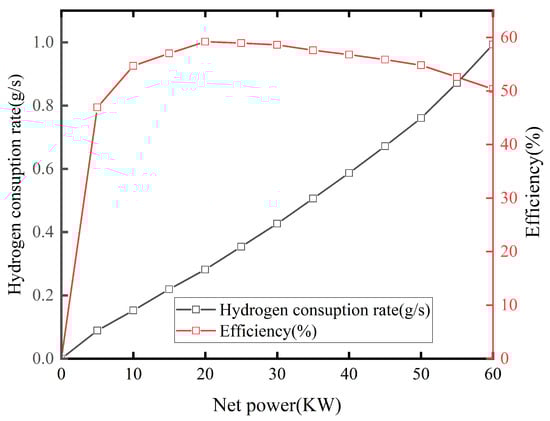
Figure 2. Net power and hydrogen consumption and efficiency curves of PEMFC.

2.3. Battery Model

Fuel cells have hysteresis and braking energy recovery failure. Consequently, the traction battery started the vehicle and implemented energy recovery as an auxiliary source. Eighty-seven single cells were cascaded to form a pack, and five packs were in a parallel connection in this work. A typical battery physical model (Figure 3) was adopted. R is the equivalent internal resistance; $V_{oc}$ is the open-circuit voltage; V is the output voltage.

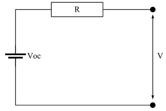
Figure 3. Battery internal-resistance model.

The SOC change rate based on the equivalent internal resistance model is

$$\dot{SOC}=-\frac{V_{oc}-\sqrt{V_{oc}^2-4R{P}_b}}{2R{Q}_b}$$

(19)

where $\dot{SOC}$ is the change rate; $P_b$ is battery power; $Q_b$ is the battery capacity.

3. Condition Classification Formulation

3.1. Conditions Data Pre-Processing

Data needed to be pre-processed due to signal distortion. Distorted condition segments were eliminated when data distortion was greater than 5 s and those less than or equal to 5 s were compensated using the mean (Equation (20)):

$$v_t=(v_{t-1}+v_{t-2})/2$$

(20)

where $v_t$ is the distortion speed; $v_{t-1}$ is the speed 1 s before distortion; $v_{t-2}$ is the speed 2 s before distortion.

Complete data after compensation were subjected to the wavelet filter. Signals contained low and high frequencies in the actual signal acquisition process, and noises were often high-frequency. Single-dimensional noise signals were expressed as

$$s\left(t\right)=f\left(t\right)+\sigma e\left(t\right)t=0,1,2,\dots n$$

(21)

where $s\left(t\right)$ is the primary signal; $f\left(t\right)$ is the actual signal; $\sigma$ is the noise standard deviation; $e\left(t\right)$ is the noise. The wavelet denoising process first decomposes the original signal and then uses threshold processing for each layer. Finally, the signals of each layer were reconstructed. Soft-threshold signal processing (Equation (22)) was selected in this work.

$$w\lambda =\left\{\begin{array}{cc}\left[sign\right(w\left)\right]\left(\right|w|-\lambda )& \left|w\right|\ge \lambda \\ 0& \left|w\right|<\lambda \end{array}\right.$$

(22)

where w is the wavelet coefficient; $\lambda$ is the threshold. When the absolute value of the wavelet coefficient was equal to a given threshold value, the soft threshold value was subtracted from the threshold value; when it was less than the given threshold value, the soft threshold value was 0. Figure 4 illustrates a part of the pre-processed data due to the large data size. Data were smoother with a smaller fluctuation frequency.

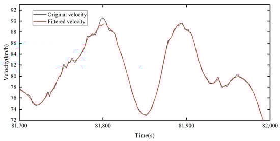
Figure 4. Comparison between parts of the collected data before and after processing.

3.2. Classification of Working Conditions

Pre-processed data were constructed for short-stroke working conditions, and the short-stroke eigenvalues were selected for PCA. This was to reduce the feature dimensionality and improve the classification. Finally, K-means clustering was used.

Each short-stroke segment included an idle speed segment, an accelerating segment, a decelerating segment, and a uniform speed segment in the construction of the short-stroke conditions. The preliminary screening process for short-stroke working conditions was as follows:

Step 1: There was inevitably a long-term parking state during the implementation due to the long data measurement time. The state did not meet the requirements of the cycle working conditions, so the idle speed segment of >200 s was reduced to 200 s.

Step 2: The acceleration did not exceed 5 m/s² in the process of matching the dynamics of the vehicle since a commercial vehicle was used in the work. Therefore, the short stroke containing acceleration greater than 5 m/s² was excluded.

The selection of too many eigenvalues was not conducive to the identification of working conditions, and it was easy to cause dimensional errors. The eigenvalues selected in this work are as follows, according to Refs. [33,34]: the maximum speed ($v_{max}$), average speed ($\overline{v}$), average operating speed (${\overline{v}}_{run}$), operating ratio ($r_{run}$), parking ratio ($r_s$), maximum acceleration ($a_{max}$), average acceleration of the acceleration segment ($\overline{a}$), acceleration ratio ($r_a$), maximum deceleration ($d_{max}$), average deceleration of the deceleration segment ($\overline{d}$), and deceleration ratio ($r_d$).

A large classification error occurred if the eigenvalues were directly classified by K-means because each eigenvalue has a certain correlation. Therefore, principal component analysis (PCA) needed to be first used for data dimensionality reduction before K-means classification.

The PCA data dimension-reduction method maps the high-latitude feature parameters to the low-latitude counterparts and replaces the original data feature parameters with fewer feature parameters (principal components) without losing the original data feature parameters. The observation sample matrix is as follows:

$$X_{m \times n}=\left[\begin{array}{cccc}{x}_{11}& x_{12}& \dots & x_{1n}\\ x_{21}& x_{22}& \dots & x_{2n}\\ ⋮& ⋮& ⋮& ⋮\\ x_{m1}& x_{m2}& \dots & x_{mn}\end{array}\right]$$

(23)

where $X_{m \times n}$ is the original observation data; m is the number of data samples; n is the feature parameters. The feature parameters of the original data needed to be standardized to prevent different feature dimensions from affecting the data. Standardized data are $Z_{m \times n}$, and the elements in the standardized data could be obtained from Equations (24)–(26). $i\le m$ and $j\le n$; both are integers.

$$Z_{ij}=\frac{x_{ij}-{\dot{x}}_j}{s_j}$$

(24)

$${\overline{x}}_j=\frac{1}{m}\sum _{i=1}^m{x}_{ij}$$

(25)

$$s_j=\sqrt{\frac{1}{m-1}\sum _{i=1}^m{(x_{ij}-{\dot{x}}_j)}^2}$$

(26)

Then, the correlation coefficient matrix $R_{mn}$ of $Z_{mn}$ was calculated, and element $r_{ij}$ in $R_{mn}$ could be obtained by

$$r_{ij}=\frac{{\sum }_{k=1}^m(Z_{ki}-{\overline{Z}}_i)(Z_{kj}-{\overline{Z}}_j)}{\sqrt{{\sum }_{k=1}^m{(Z_{ki}-{\overline{Z}}_i)}^2{(Z_{kj}-{\overline{Z}}_j)}^2}}$$

(27)

$$R_{m \times n}=\left[\begin{array}{cccc}{r}_{11}& r_{12}& \dots & r_{1n}\\ r_{21}& r_{22}& \dots & r_{2n}\\ ⋮& ⋮& ⋮& ⋮\\ r_{m1}& r_{m2}& \dots & r_{mn}\end{array}\right]$$

(28)

The eigenvalues and eigenvectors of $R_{mn}$ could be obtained by calculating the sum, and then n eigenvalues could be obtained accordingly. They were arranged from large to small: $a_1\ge a_2\ge a_3\dots a_n\ge 0$. Eigenvalue $a_j$ was substituted into the following calculation equation to obtain the contribution rate ${\beta }_j$ of the jth principal component and cumulative contribution rate $\beta \left(j\right)$ of the previous j principal components. The appropriate principal components were selected according to the contribution rate of each principal component and the cumulative contribution rate:

$${\beta }_j=\frac{a_j}{{\sum }_{j=1}^n{a}_j}$$

(29)

$$\beta \left(j\right)=\frac{{\sum }_{k=1}^j{a}_k}{{\sum }_{k=1}^n{a}_k}$$

(30)

The relationship between the principal component, the contribution rate, and the cumulative contribution rate (Figure 5) could be obtained through Equations (23)–(30). The cumulative contribution rate was 85.60% when the principal component was number 3. Therefore, the first three principal components were selected for K-means clustering analysis in this work.

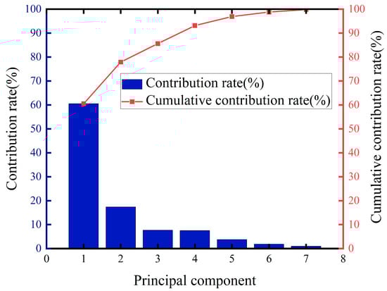
Figure 5. Relationship between the principal component, contribution rate, and the cumulative contribution rate.

The K-means algorithm is an iterative solution optimization algorithm. It solves the Euclidean distance between the sample data and the cluster center and divides them into different categories according to the distance from each cluster center. The K-means solution process is as follows:

Step 1: Select the number of clustering (K), and randomly select K clustering center points.

Step 2: Calculate the distance between each sample data point and the clustering center, and divide the sample data into the samples closest to the clustering center according to the distance.

Step 3: The mean value of each cluster is calculated and taken as a new clustering center point.

Step 4: Determine whether the clustering center has changed. If so, repeat Steps 2 and 3. If not, end the operation.

Step 5: The classification results are obtained.

The number of clusters selected in this work was four from the above steps. Figure 6 shows the classification results for the short-stroke working conditions.

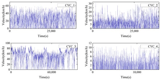
Figure 6. Short-stroke condition classification results.

$CYC\_1$ conforms to the suburban dredging conditions, with its maximum speed hovering at 60 km/h, low start–stop times, and few idle speed segments. $CYC\_2$ conforms to urban dredging conditions, with its maximum speed hovering at 30 km/h, low start–stop times, and few idle speed segments. $CYC\_3$ conforms to high-speed working conditions, with its maximum speed hovering at 90 km/h, lower start–stop times, and fewer idle speed segments. $CYC\_4$ conforms to urban congestion conditions, with its maximum speed hovering at 10 km/h, more start–stop times, and more idle speed segments. Therefore, the difference in each working condition is obvious.

4. Strategy Framework of Energy Management Predicted by the Adaptive Model

Figure 7 shows the strategy framework of energy management predicted by the adaptive model in this work. The entire EMS was divided into an offline processing area and online control area. The driving condition data of the vehicle were obtained by GPS, and four working condition categories were obtained through the pre-processing of the original data, short-stroke division, PCA, and K-means clustering in the offline processing area. The RBFNN was used to train the data under each working condition category, so the speed prediction controller under each working condition was obtained.

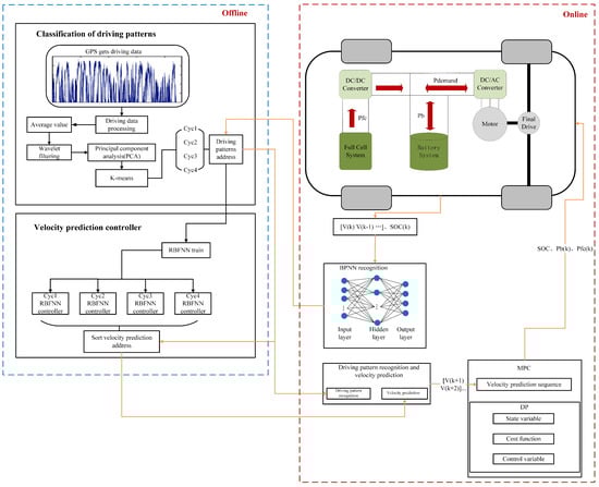
Figure 7. Control framework for the devised predictive energy management strategy.

The vehicle extracted historical speed data in the online area during operation, and the BPNN was used to identify the current and future working condition categories in the time domain and obtain the speed prediction controller of the corresponding working conditions. Finally, the MPC was used to allocate the two energy sources in real time. MPC could obtain the locally optimal control sequence of working conditions based on model prediction, rolling optimization, and feedback correction, and the first control sequence was applied to the vehicle. The MPC energy management strategy in this work used RBFNN as a prediction model and DP as a solver to solve the optimal control sequence.

4.1. Working Condition Identification

The BPNN is a multi-layer feedforward network and uses error backpropagation, with a good effect on category recognition. The BPNN is composed of the input layer, hidden layer, and output layer (Figure 8).

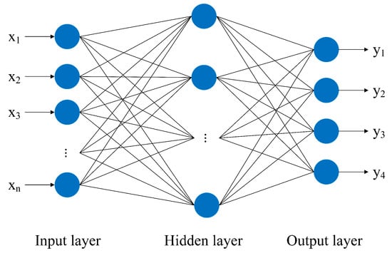
Figure 8. Back propagation neural network (BPNN) structure.

$x_1,x_2,x_3,\dots$, and $x_n$ are the input of the neural network; $y_1,y_2,y_3,y_4$ are the output of the neural network. The BPNN training process is as follows:

Step 1: First determine the number of input layers, hidden layers, and output layers of the neural network, and initialize the threshold value between the layers.

Step 2: Calculate the output value of the hidden layer and that of the output layer. The calculation formula is as follows:

$$H_j=f(\sum _{i=1}^n{w}_{ij}{x}_i-{\theta }_j)j=1,2,3,\dots ,l$$

(31)

$$O_k=\sum _{j=1}^l{H}_j{w}_{jk}-b_{k}k=1,2,3,\dots ,m$$

(32)

where $H_j$ is the output value of the hidden layer; f is the activation function of the hidden layer; l is the number of nodes of the hidden layer; $w_{ij}$ and $w_{jk}$ are the weight of the neural network; ${\theta }_j$ is the threshold value of the hidden layer; $O_k$ is the output value of the output layer; $b_k$ is the threshold value of the output layer; m is the number of nodes of the output layer.

Step 3: Calculate the error value.

$$e_k=Y_k-O_k$$

(33)

Step 4: Use the gradient descent method to adjust the threshold value.

$$w_{ij}=w_{ij}+\eta H_j(1-H_j)x\left(i\right)\sum _{k=1}^n{w}_{jk}{e}_k$$

(34)

$$w_{jk}=w_{jk}-\eta e_k{H}_j$$

(35)

Step 5: Calculate the new threshold.

$${\theta }_k={\theta }_k+\eta H_j\sum _{k=1}^n{w}_{jk}{e}_k$$

(36)

$$b_k=b_k-\eta e_k$$

(37)

Historical working condition data $[v_{k-C{H}_h+1},v_{k-C{H}_h+2},\dots ,v_k]$ were collected to calculate the 11 feature parameters in Section 3.2, and identify the future working condition categories of $[v_{k+1},v_{k+2},\dots ,v_{k+C{H}_p}]$ in the BPNN training process. $C{H}_h$ is the length of historical sampling data, and $C{H}_p$ is the length of the working condition prediction. The BPNN output layer was changed to a binary category. (1 0 0 0), (0 1 0 0), (0 0 1 0), and (0 0 0 1) were output for categories 1–4, respectively. The binary output results were reversed to solve the category.

4.2. Construction of the Rule-Based Energy Management Strategy

Rule-based construction was used to verify the superiority of the self-adaptive model predictive energy management strategy in this section. The multi-point control energy management strategy was constructed in this work, and the fuel cell was fixed on multi-point power. Fuel-cell power was adjusted in real time according to the power cell SOC and the required power. Figure 9 shows the flow of the energy management strategy of the multi-point control rules.

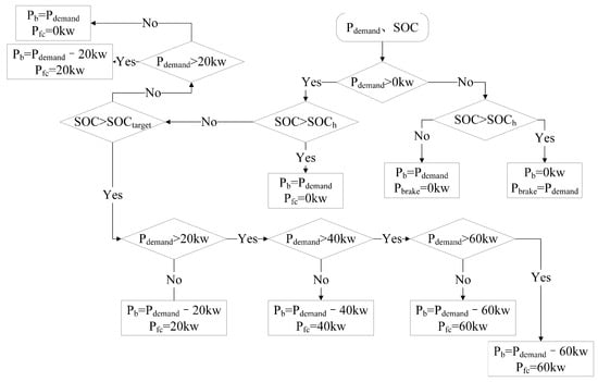
Figure 9. Rule-based EMS.

In Figure 9, $P_{demand}$ is the required power; $SO{C}_h$ and SOCtarget are the highest SOC value and target value of the cell, respectively; $P_{fc}$ is fuel-cell power; $P_{brake}$ is braking power. When $P_{demand}<0$, the vehicle is braking. If the SOC is greater than the maximum limit, no braking energy recovery will be carried out, and all braking force will be mechanically braked. When $P_{demand}<0$, the cell SOC needs to be judged. When $SOC>SO{C}_h$, the required power is provided by the power cell. When the SOC is small, the fuel cell and the power cell jointly increase the required power.

4.3. RBFNN Velocity Prediction

RBFNNs are divided into the input layer, hidden layer, and output layer. Unlike the BPNN, the RBFNN is a feedforward neural network. The hidden layer contains radial basis functions, and the training velocity is fast. In addition, it is not easy to fall into local optimum. Therefore, a higher accuracy can be achieved using RBFNN velocity prediction. The radial basis function selected in this work is as follows:

$$\alpha \left(x\right)=exp(-\frac{{∥x-u_t∥}^2}{{\sigma }_t^2})$$

(38)

where $u_t$ is the center point; ${\sigma }_t$ is the radial base width. The root mean square error (RMSE) was selected as the evaluation index, and the equation is as follows:

$$RMSE\left(K\right)=\sqrt{\frac{{\sum }_{K=1}^{t_p}{(v(k+i)-v_0(k+i))}^2}{t_p}}$$

(39)

$$RMSE=\frac{{\sum }_{k=1}^{n}RMSE\left(k\right)}{n}$$

(40)

where $RMSE\left(k\right)$ is the root mean square error in the prediction time domain of the kth sampling point; n is the number of sampling points; $t_p$ is the length of the prediction time. The 10-60-$H_p$ RBFNN structure was constructed, and $H_p$ was the predicted time domain length. The RBFNN velocity predictors in category 5 were constructed here, using the pre-processed data in Section 3.1 and Section 3.2: $CYC1$-4. In total, 70% of each type of data was taken as the training set and 30% as the test set, and the RBFNN velocity predictor of category 5 was constructed.

4.4. DP

The entire system solves the constrained problems in the finite time domain by predicting the future velocity, so DP was used as the finite time domain solver. DP contains the state variables, control variables, objective functions, and constraints.

The SOC and the power distribution factor were taken as state variables and control variables, and the state variables were discretized.

$$x_{k+1}=f_k(x_k,u_k)k=0,1,2,\dots ,N$$

(41)

where $x_{k+1}$ is the state variable at k + 1 time; $f_k$ is the state transition equation; $u_k$ is the control variable. The control variable is the fuel-cell power in this work; N is the driving cycle length. The state transition equation is as follows:

$$SOC(k+1)=SOC\left(k\right)-\frac{V-\sqrt{V^2-4R(P_{demand}\left(k\right)-P_{fc}\left(k\right))}}{2RQ}$$

(42)

where V is the open-circuit voltage of the power battery. The objective function is as follows:

$$J=min\sum _{t=k}^{k+p}(\alpha {\dot{m}}_{H2}+\beta {∥SOC\left(t\right)-SO{C}_{taget}∥}^2)$$

(43)

The constraints are as follows:

$$\left\{\begin{array}{c}SO{C}_{min}\le SOC\left(k\right)\le SO{C}_{max}\\ P_{fc\_min}\le P_{fc}\left(k\right)\le P_{fc\_max}\\ P_{b\_min}\le P_b\left(k\right)\le P_{b\_max}\end{array}\right.$$

(44)

where $SO{C}_{min}$ is the minimum SOC limit (0.3); $SO{C}_{max}$ is the maximum SOC limit (0.8); $P_{fc\_min}$ is the minimum power of the fuel cell; $P_{fc\_max}$ is the maximum power of the fuel cell; $P_{b\_min}$ is the maximum charging power of the power battery; $P_{b\_max}$ is the maximum discharge power of the power battery.

5. Simulation and Result Discussion

The simulation was performed in MATLAB 2021b on a laptop with the configurations of Inter Core i9-12900H CPU @ 2.50 GHz. This section discusses the BPNN recognition accuracy and velocity prediction optimization accuracy and the performance of the proposed EMS. In addition, the self-adaptive EMS is compared with the rules and dynamic planning, and the SOC change curve and hydrogen consumption are analyzed.

5.1. Working Condition Recognition and Analysis

The recognition sampling time was 150 s in the work, and the sampling data were calculated as 11 eigenvalues in Section 3.2, which were used as BPNN data. The binary working condition in category 4 was used as the output of the neural network. The length of the predicted working condition was 5 s. In total, 60% of the short-stroke fragments were used as a training set, 20% were used as a test set, and 10% were used as a verification set. Figure 10 shows the comparison before and after the verification results. The BPNN recognition accuracy reached 97.5%, and a good recognition effect was achieved by the trained BPNN.

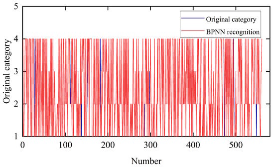
Figure 10. Comparison between BPNN recognition verification sets.

5.2. Velocity Prediction Analysis

The RBFNN speed prediction was optimized by the online identification of working conditions. RBFNN predictors under the corresponding working conditions were selected using the online recognition of working conditions to achieve the self-adaptive prediction effect. The typical working conditions of WTVC were used to verify the advantages and disadvantages of the optimized velocity in this section. The WTVC working conditions included urban, suburban, and high-speed, which made the verification results more representative.

First, the BPNN was used to identify the WTVC working conditions. Figure 11 shows the working condition recognition curve and the WTVC graph. Secondly, the corresponding working condition RBFNN velocity predictor was retrieved. Historical data collected in the RBFNN velocity prediction were for 10 s, and the prediction lengths were 5, 10, 15, and 20 s in this work. Figure 12 shows the comparison of velocity prediction before and after optimization, and Table 4 presents the RMSE statistics of velocity prediction before and after optimization.

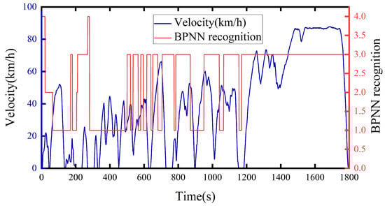
Figure 11. WTVC and BPNN recognition.

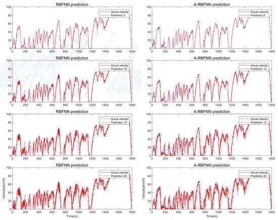
Figure 12. Comparison between the velocity prediction of RBFNN and A-RBFNN.

Table 4. Comparison of velocity prediction accuracy.

RMSE	Prediction Lengths
	5 S	10 S	15 S	20 S
RBFNN	1.806	3.653	5.452	7.206
A-RBFNN	1.53	3.42	5.43	7.182
Improvement	9.75%	6.38%	0.40%	0.33%

The prediction accuracy of the A-RBFNN (the adaptive RBFNN) was higher than that of the RBFNN, and the accuracy of the A-RBFNN relative to the RBFNN increased the most when the speed was at 5 s, with an increase of 9.75% (Table 4). Therefore, 5 s was selected as the optimal prediction length in this work.

5.3. Predictive Energy Management of the Self-Adaptive Model

The WTVC was selected as the driving cycle to verify the working conditions in this work. The energy management strategy predicted by the self-adaptive model was compared with dynamic planning and rule-based strategies. Then, the advantages of the proposed strategy were discussed. The initial SOC value was 0.6 and $SO{C}_{target}$ was 0.6 in this section. The RBFNN was selected to predict the time domain length as 5 s according to the analysis in Section 5.2. Figure 13 shows the SOC variation trend in the DP energy management strategy, the rule-based energy management strategy, and the self-adaptive model prediction of the energy management strategy.

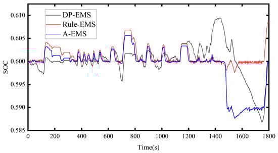
Figure 13. Comparison of SOC in each EMS.

The proposed A-EMS (the adaptive energy management strategy) had a smaller frequency change than the SOC in the Rule-EMS (the rule energy management strategy), which prolonged the service life of the power battery, and the A-EMS was able to follow the target SOC value well (Figure 13).

The A-EMS was able to follow the SOC target value well in the end, and the final SOC value reached 0.601 (Table 5). The equivalent hydrogen consumption rates of Rule-EMS and A-EMS were 92.9% and 96.4%, respectively, compared with the DP-EMS (the dynamic programming energy management strategy), and the fuel economy was improved by 3.5%.

Table 5. Simulation results of EMS.

EMS	C${}_{\mathit{H}2}$	SOC${}_{\mathit{end}}$	E-C${}_{\mathit{H}2}$
DP-based	544.470	0.600	544.470
Rule-based	585.967	0.608	585.807
A-EMS-based	565.005	0.601	565.005

6. Conclusions

A self-adaptive model prediction energy management strategy was proposed in this work, The combination of working condition recognition with MPC produces the adaptive effect. Using GPS data from real vehicles, the working condition classification (the urban decongestion condition, urban congestion condition, suburban condition, and highway condition) was built using PCA and K-means. The RBFNN speed predictor was trained under each condition while taking into account the effect of condition classification on speed prediction, and the RBFNN speed prediction method is proposed for online BPNN condition recognition. The problem of frequent SOC fluctuation was tackled by employing DP as an MPC solver and one of the cost functions as the rate of change of the SOC.

The simulation results validated the efficacy of the designed EMS. The recognition accuracy of the working condition classification and BPNN recognition according to data obtained from an actual vehicle was 97.5%. At a 5s prediction length, the combination of online BPNN recognition and RBFNN speed prediction using BPNN resulted in a 9.75% improvement in the overall speed prediction accuracy. Secondly, it reduced hydrogen consumption by 3.5% and reduced the frequency of SOC fluctuations compared to the rule-based strategy. Furthermore, the proposed strategy’s performance is close to that of the offline DP, indicating that it is close to the optimal effect. In the future, fuel-cell lifetime will be treated as a cost function to reduce fuel-cell overuse scenarios and to use variable time domain models to predict energy management strategies.

References

- Guo, Z.; Sun, S.; Wang, Y.; Ni, J.; Qian, X. Impact of New Energy Vehicle Development on China’s Crude Oil Imports: An Empirical Analysis. World Electr. Veh. J. 2023, 14, 46. [Google Scholar] [CrossRef]
- Zhang, Z.; Dong, R.; Lan, G.; Yuan, T.; Tan, D. Diesel particulate filter regeneration mechanism of modern automobile engines and methods of reducing PM emissions: A review. Environ. Sci. Pollut. Res. Int. 2023, 30. [Google Scholar] [CrossRef] [PubMed]
- Tan, D.; Meng, Y.; Tian, J.; Zhang, C.; Zhang, Z.; Yang, G.; Cui, S.; Hu, J.; Zhao, Z. Utilization of renewable and sustainable diesel/methanol/n-butanol (DMB) blends for reducing the engine emissions in a diesel engine with different pre-injection strategies. Energy 2023, 269. [Google Scholar] [CrossRef]
- Zhang, Z.; Dong, R.; Tan, D.; Duan, L.; Jiang, F.; Yao, X.; Yang, D.; Hu, J.; Zhang, J.; Zhong, W.; et al. Effect of structural parameters on diesel particulate filter trapping performance of heavy-duty diesel engines based on grey correlation analysis. Energy 2023, 271. [Google Scholar] [CrossRef]
- Zhao, X.; Wang, L.; Zhou, Y.; Pan, B.; Wang, R.; Wang, L.; Yan, X. Energy management strategies for fuel cell hybrid electric vehicles: Classification, comparison, and outlook. Energy Convers. Manag. 2022, 270, 116179. [Google Scholar] [CrossRef]
- Wu, J.; Zhang, N.; Tan, D.; Chang, J.; Shi, W. A robust online energy management strategy for fuel cell/battery hybrid electric vehicles. Int. J. Hydrog. Energy 2020, 45, 14093–14107. [Google Scholar] [CrossRef]
- Sulaiman, N.; Hannan, M.; Mohamed, A.; Ker, P.J.; Majlan, E.; Daud, W.W. Optimization of energy management system for fuel-cell hybrid electric vehicles: Issues and recommendations. Appl. Energy 2018, 228, 2061–2079. [Google Scholar] [CrossRef]
- Sorlei, I.-S.; Bizon, N.; Thounthong, P.; Varlam, M.; Carcadea, E.; Culcer, M.; Iliescu, M.; Raceanu, M. Fuel cell electric vehicles—A brief review of current topologies and energy management strategies. Energies 2021, 14, 252. [Google Scholar] [CrossRef]
- Li, J.-q.; Fu, Z.; Jin, X. Rule Based Energy Management Strategy for a Battery/Ultra-capacitor Hybrid Energy Storage System Optimized by Pseudospectral Method. Energy Procedia 2017, 105, 2705–2711. [Google Scholar] [CrossRef]
- Du, C.; Huang, S.; Jiang, Y.; Wu, D.; Li, Y. Optimization of energy management strategy for fuel cell hybrid electric vehicles based on dynamic programming. Energies 2022, 15, 4325. [Google Scholar] [CrossRef]
- Wang, Y.; Sun, Z.; Chen, Z. Rule-based energy management strategy of a lithium-ion battery, supercapacitor and PEM fuel cell system. Energy Procedia 2019, 158, 2555–2560. [Google Scholar] [CrossRef]
- Wang, Y.; Zhang, Y.; Zhang, C.; Zhou, J.; Hu, D.; Yi, F.; Fan, Z.; Zeng, T. Genetic algorithm-based fuzzy optimization of energy management strategy for fuel cell vehicles considering driving cycles recognition. Energy 2023, 263, 126112. [Google Scholar] [CrossRef]
- Wang, Y.; Sun, Z.; Chen, Z. Development of energy management system based on a rule-based power distribution strategy for hybrid power sources. Energy 2019, 175, 1055–1066. [Google Scholar] [CrossRef]
- Min, X.; Haidong, S.; Darren, W.; Siliang, L.; Lei, S.; de Silva, C.W. Intelligent Fault Diagnosis of Machinery Using Digital Twin-assisted Deep Transfer Learning. Reliab. Eng. Syst. Saf. 2021, 215, 107938. [Google Scholar]
- Xiao, Y.; Shao, H.; Han, S.; Huo, Z.; Wan, J. Novel Joint Transfer Network for Unsupervised Bearing Fault Diagnosis From Simulation Domain to Experimental Domain. IEEE/ASME Trans. Mechatronics 2022, 27, 5254–5263. [Google Scholar] [CrossRef]
- Chen, M.; Shao, H.; Dou, H.; Li, W.; Liu, B. Data Augmentation and Intelligent Fault Diagnosis of Planetary Gearbox Using ILoFGAN Under Extremely Limited Samples. IEEE Trans. Reliab. 2022, 1–9. [Google Scholar] [CrossRef]
- Li, W.; Ye, J.; Cui, Y.; Kim, N.; Cha, S.W.; Zheng, C. A speedy reinforcement learning-based energy management strategy for fuel cell hybrid vehicles considering fuel cell system lifetime. Int. J. Precis. Eng. Manuf. Green Technol. 2021, 9, 859–872. [Google Scholar] [CrossRef]
- Dong, P.; Zhao, J.; Liu, X.; Wu, J.; Xu, X.; Liu, Y.; Wang, S.; Guo, W. Practical application of energy management strategy for hybrid electric vehicles based on intelligent and connected technologies: Development stages, challenges, and future trends. Renew. Sustain. Energy Rev. 2022, 170, 112947. [Google Scholar] [CrossRef]
- Shao, H.; Li, W.; Cai, B.; Wan, J.; Xiao, Y.; Yan, S. Dual-Threshold Attention-Guided Gan and Limited Infrared Thermal Images for Rotating Machinery Fault Diagnosis Under Speed Fluctuation. IEEE Trans. Ind. Inform. 2023, 1–10. [Google Scholar] [CrossRef]
- Dreyfus, S. Richard Bellman on the birth of dynamic programming. Operations Research 2002, 50, 48–51. [Google Scholar] [CrossRef]
- Kandidayeni, M.; Macias, A.; Boulon, L.; Kelouwani, S. Efficiency upgrade of hybrid fuel cell vehicles’ energy management strategies by online systemic management of fuel cell. IEEE Trans. Ind. Electron. 2020, 68, 4941–4953. [Google Scholar] [CrossRef]
- Liu, Y.; Liang, J.; Song, J.; Ye, J. Research on Energy Management Strategy of Fuel Cell Vehicle Based on Multi-Dimensional Dynamic Programming. Energies 2022, 15, 5190. [Google Scholar] [CrossRef]
- Gao, H.; Wang, Z.; Yin, S.; Lu, J.; Guo, Z.; Ma, W. Adaptive real-time optimal energy management strategy based on equivalent factors optimization for hybrid fuel cell system. Int. J. Hydrogen Energy 2021, 46, 4329–4338. [Google Scholar] [CrossRef]
- Zou, P.; Tao, F.; Fu, Z.; Si, P.; Ma, C. Optimal energy management strategy for fuel cell/battery/supercapacitor vehicles using wavelet transform and equivalent consumption minimization strategy. Proc. Inst. Mech. Eng. Part D J. Automob. Eng. 2022, 236, 3168–3178. [Google Scholar] [CrossRef]
- Huang, Y.; Wang, H.; Khajepour, A.; He, H.; Ji, J. Model predictive control power management strategies for HEVs: A review. J. Power Sources 2017, 341, 91–106. [Google Scholar] [CrossRef]
- Rezzak, D.; Boudjerda, N. Management and control strategy of a hybrid energy source fuel cell/supercapacitor in electric vehicles. Int. Trans. Electr. Energy Syst. 2017, 27, e2308. [Google Scholar] [CrossRef]
- Zhou, Y.; Ravey, A.; Péra, M.-C. Multi-mode predictive energy management for fuel cell hybrid electric vehicles using Markov driving pattern recognizer. Appl. Energy 2020, 258, 114057. [Google Scholar] [CrossRef]
- Yan, M.; Cheng, L.; Siyu, W. Multi-objective energy management strategy for fuel cell hybrid electric vehicle based on stochastic model predictive control. ISA Trans. 2022, 131, 178–196. [Google Scholar]
- Hu, J.; Liu, D.; Du, C.; Yan, F.; Lv, C. Intelligent energy management strategy of hybrid energy storage system for electric vehicle based on driving pattern recognition. Energy 2020, 198, 117298. [Google Scholar] [CrossRef]
- Mat, I.Z.; Mohd, N.N.; Hafiz, A.M.; Mohamad, K.N.A. Optimizing PEMFC model parameters using ant lion optimizer and dragonfly algorithm: A comparative study. Int. J. Electr. Comput. Eng. (IJECE) 2019, 9, 5312–5320. [Google Scholar]
- Khan, M.; Iqbal, M. Modelling and analysis of electro-chemical, thermal, and reactant flow dynamics for a PEM fuel cell system. Fuel Cells 2005, 5, 463–475. [Google Scholar] [CrossRef]
- Pukrushpan, J.T.; Peng, H.; Stefanopoulou, A.G. Control-oriented modeling and analysis for automotive fuel cell systems. J. Dyn. Sys. Meas. Control 2004, 126, 14–25. [Google Scholar] [CrossRef]
- Liu, D.; Zhang, J.; Li, X.; Quan, L.; Hu, X.; Xing, K. Research on the Construction Method of Driving Conditions with Optimal Deviation Based on Fuzzy C-Means Clustering. J. Phys. Conf. Ser. 2022, 2400, 012023. [Google Scholar] [CrossRef]
- Langari, R.; Jong-Seob, W. Intelligent energy management agent for a parallel hybrid vehicle-part I: System architecture and design of the driving situation identification process. IEEE Trans. Veh. Technol. 2005, 54, 925–934. [Google Scholar] [CrossRef]
Disclaimer/Publisher’s Note: The statements, opinions and data contained in all publications are solely those of the individual author(s) and contributor(s) and not of MDPI and/or the editor(s). MDPI and/or the editor(s) disclaim responsibility for any injury to people or property resulting from any ideas, methods, instructions or products referred to in the content. |
© 2023 by the authors. Licensee MDPI, Basel, Switzerland. This article is an open access article distributed under the terms and conditions of the Creative Commons Attribution (CC BY) license (https://creativecommons.org/licenses/by/4.0/).