A Novel WD-SARIMAX Model for Temperature Forecasting Using Daily Delhi Climate Dataset

Abstract

Forecasting is defined as the process of estimating the change in uncertain situations. One of the most vital aspects of many applications is temperature forecasting. Using the Daily Delhi Climate Dataset, we utilize time series forecasting techniques to examine the predictability of temperature. In this paper, a hybrid forecasting model based on the combination of Wavelet Decomposition (WD) and Seasonal Auto-Regressive Integrated Moving Average with Exogenous Variables (SARIMAX) was created to accomplish accurate forecasting for the temperature in Delhi, India. The range of the dataset is from 2013 to 2017. It consists of 1462 instances and four features, and 80% of the data is used for training and 20% for testing. First, the WD decomposes the non-stationary data time series into multi-dimensional components. That can reduce the original time series’ volatility and increase its predictability and stability. After that, the multi-dimensional components are used as inputs for the SARIMAX model to forecast the temperature in Delhi City. The SARIMAX model employed in this work has the following order: (4, 0, 1). (4, 0, [1], 12). The experimental results demonstrated that WD-SARIMAX performs better than other recent models for forecasting the temperature in Delhi city. The Mean Square Error (MSE), Mean Absolute Error (MAE), Median Absolute Error (MedAE), Root Mean Square Error (RMSE), Mean Absolute Percentage Error (MAPE), and determination coefficient ($R^2$) of the proposed WD-SARIMAX model are 2.8, 1.13, 0.76, 1.67, 4.9, and 0.91, respectively. Furthermore, the WD-SARIMAX model utilized the proposed to forecast the temperature in Delhi over the next eight years, from 2017 to 2025.

1. Introduction

Humanity faces a formidable obstacle in the form of climate change mitigation. Forecasting climate change’s impact on the planet is difficult, but scientists agree that it will have severe consequences. Temperature extremes, ecosystem alteration, biodiversity loss, soil erosion, rising sea levels, and global warming are only some of the problems that have been documented [1]. Due to the challenges of reaching a high level of accuracy in temperature forecasting, this area, in general, has become a key field for implementing Machine Learning (ML) methods [2,3]. For example, it has been shown that temperature data series exhibit nonlinear behavior and nontrivial long-scope correlations in their volatility [4]. Furthermore, these time series have substantial regional, seasonal, and temporal diversity [5]. With empirical methodologies, temperature forecasting can be estimated [6,7]. Most follow quality standards and reasonable procedures, which is why they are so accurate and reliable.

The Auto-Regressive Integrated Moving Average (ARIMA) approach is one of the most cost-effective and reliable time series. It stabilizes data by minimizing variances and decomposing data to extract components, including seasonality, residuals, trends, and analyses of associations between parameters. ARIMA with exogenous variables is called ARIMAX, and the seasonal ARIMA is called SARIMA are all examples of ARMA-extend models that have their perks, but the former is better at considering seasonality in data, while the latter is better at accounting for external influences [8].

1.1. Prior Works on Temperature Forecasting

Jenny Cifuentes [9] provided machine learning strategies for forecasting weather conditions, such as temperature and humidity levels, using a variety of input factors, such as historical data on these variables and others like solar radiation, precipitation, and wind speed. The analysis showed that deep learning techniques reported lower errors than conventional artificial neural network designs. They favored Support Vector Machines (SVM) worldwide because they struck an excellent balance between ease of use and precision. Authors in [10] utilized Myitkyina’s yearly temperature forecasts from 2010–2017 using the Prophet prediction technique. By considering the impact of unique holidays and seasonality, Prophet was a modular regression approach that made highly accurate predictions across time sequences using just a few parameters. The approach’s prediction accuracy was evaluated using the Root Mean Square Error (RMSE), which was 5.7573 in both 2012 and 2013. Nengbao Liu et al. [11] suggested two models, Neural Network and SARIMAX, to forecast temperature-driven power usage. When developing the SARIMAX approach, the “pre-whitening” technique was utilized to calculate the lagging impact of temperature on power demand. Even though Neural Network’s MAPE and RMSE were lower than SARIMAX’s during the estimate phase, it was still unable to outperform SARIMAX over the forecasting period of one week. Hui Zhang et al. [12] presented three machine learning (ML) methods (LSTM-FCN, Linear Regression, and LightGBM) to forecast the temperature of a high-resolution operating method called GRAPES-3km. Predictions and observations for 2019 and 2020 in Shaanxi province, China, were used as input variables. LightGBM outperformed the other two approaches, with a prediction accuracy of over 84%. Zao Zhang and Yuan Dong [13] developed a neural network method to extrapolate future temperature readings from existing ones. They created a model for a convolutional recurrent neural network (CRNN) that combined the strengths of CNNs and RNNs. The model studied past data and understood the spatial and temporal relationships between temperature changes. The suggested CRNN model was tested using a dataset consisting of daily temperatures recorded throughout mainland China between 1952 and 2018. Arpan Nandi. [14] proposed an ALTF Net model (Attention-based Long term Temperature Forecasting Network) for long-term temperature forecasting using an Encoder-Decoder orientation. The Encoder encodes the auto-regressive time series’ relative dependencies into an attention tensor, which is then utilized by the Decoder to generate the prediction. A convolution block is added to the Encoder to help it understand seasonal trends. In contrast to RNN and LSTM, the suggested model ALTF employs a Transformer with an enhanced encoder to forecast temperatures up to 150 days with good accuracy.

1.2. Paper Contribution

The main contribution of this study is to develop a systematic framework that combines Temperature Forecasting (TS) modeling techniques, and Machine Learning (ML) approaches for forecasting the temperature in Delhi city. Firstly, the TS modeling is discussed, and the recognition tasks are performed secondly. The performance of the proposed framework was validated using data from a daily Delhi climate time series dataset. The augmented Dickey-Fuller (ADF) test and correlogram analysis are involved in checking for the presence of a seasonal unit root. To ensure the stationarity of the time series, respectively. To relax the stationarity requirement, the SARIMAX model was introduced, accompanied by the model parameter selection criteria and a candidate model mechanism. In the classification module, multiple ML classifiers, for example, Extra Trees (ET) Regressor, Dummy Regressor (DR), Elastic Net (EN) Regressor, Bayesian Ridge (BR) Regressor, and Lasso Regressor (LR), were engaged. Mean Absolute Percentage Error (MAPE), Mean Squared Error (MSE), Median Absolute Error (MedAE), Mean Absolute Error (MAE), Root Mean Squared Error (RMSE), and Coefficient of Determination ($R^2$) are the performance indicators used for validating the superiority of the proposed framework.

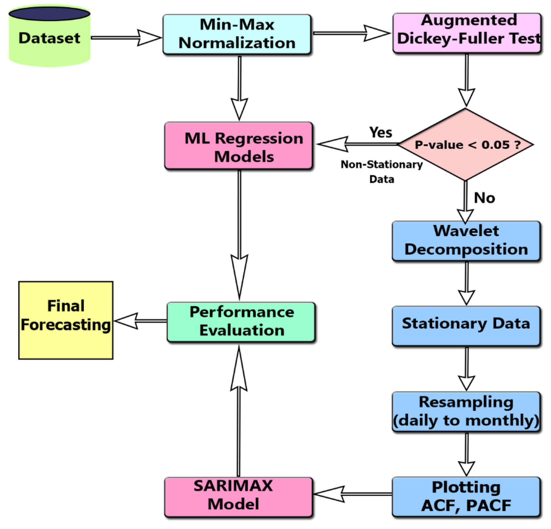
2. The Proposed Methodology

This section discusses the details of the WD-SARIMAX model for temperature forecasting using the daily Delhi climatic time series dataset and makes comparisons to several ML regression methods. Additionally, the study’s primary emphasis is a climate dataset with time series analysis that covered Delhi’s daily frequency and performed a seasonal root test. The Augmented Dickey-Fuller (ADF) test and the Correlogram analysis are involved in checking for the presence of a seasonal unit root and ensuring the time series’ stationarity. The lowest and maximum values are handled, and the range is normalized using min-max normalization. The proposed methodology combines wavelet decomposition (WD) with SARIMAX to decompose the original time series into different frequency sequences to make the data stationary. The Partial Autocorrelation Function (PACF) and Autocorrelation Function (ACF) is applied to determine the order for the SARIMAX model. Finally, the ML regression models are compared with the proposed WD-SARIMAX model, for example, Extra Trees (ET) Regressor, Dummy Regressor (DR), Elastic Net (EN) Regressor, Bayesian Ridge (BR) Regressor, and Lasso Regressor (LR). Figure 1 illustrates the proposed methodology for our research problem.

2.1. Augmented Dickey-Fuller (ADF) Test

The existence of unit roots and trends in univariate processing may be discovered from a slowly blighting autocorrelation function (ACF), which indicates non-stationarity. However, this has external power to identify the trend or unit root processes by considering the AR series, as shown in Equation (1).

$$x_t=\varphi x_{t-1}+w_t$$

(1)

if $-1<\varphi <1$, then $x_t$ is stationary. If $\varphi =1,x_t$ is not stationary; hence the unit root hypothesis is shown in Equation (2).

$$H_0:\varphi =1 \mathrm{vs.} H_1:\varphi <1$$

(2)

When $x_{t-1}$ is subtracted from (1), we get $\Delta x_t$ as in Equation (3).

$$\begin{array}{c}\hfill x_t-x_{t-1}=\varphi x_{t-1}-x_{t-1}+W_t,\\ \hfill \Delta x_t=(\varphi -1)x_{t-1}+W_t\end{array}$$

(3)

if $\delta =\varphi -1$, then $\Delta x_t$ is determined in Equation (4) as follows:

$$\Delta x_t=\delta x_{t-1}+W_t$$

(4)

Therefore, testing for $\varphi =1$ is tantamount to testing for $\delta =0$. The Augmented Dickey–Fuller (ADF) exam entails going through and evaluating three sets of models as in Equations (5) and (7).

$$\begin{array}{c}\hfill \Delta x_t=(\lambda -1)x_{t-1}+\sum _{j=1}^t{B}_j\Delta x_{t-1}+W_t\end{array}$$

(5)

$$\begin{array}{c}\hfill \Delta x_t=\alpha +(\lambda -1)x_{t-1}+\sum _{j=1}^t{B}_j\Delta x_{t-1}+W_t\end{array}$$

(6)

$$\begin{array}{c}\hfill \Delta x_t=\alpha +{\delta }_t+(\lambda -1)x_{t-1}+\sum _{j=1}^t{B}_j\Delta x_{t-1}+W_t\end{array}$$

(7)

Equation (5) represents a random walk method for AR time series with a unit root, an instance of a non-fixed time series. The drift term (intercept) is found in Equation (6), whereas the linear time trend is found in Equation (7). Most commercial time series are non-stationary because of their dynamic nature [15].

2.2. Preprocessing of Data

Normalization is a preprocessing technique used often in machine learning applications. When there is an excellent level of variation among the data, this approach attempts to process everything in a single sequence. The data is compared with several scales using mathematical functions, and data with varying scales may be transformed into a standard scale [16]. First, the lowest and maximum values are handled, and the range is normalized. The point of existence is to set the slightest value to 0 and the most significant value to 1 and to distribute all other information uniformly over this [0, 1] range. In this paper, the minimum–maximum formula, commonly called Z-score normalization, is applied as in Equation (8).

$$z=\frac{x-x_{min}}{x_{max}-x_{min}}$$

(8)

where z is the transformed data, and x is the input value. The $x_{min}$ and $x_{max}$ values are the input set’s lowest and most significant numbers.

2.3. Wavelet Decomposition (WD) and Resampling

The study of non-stationary TS has seen a dramatic uptick in popularity across various disciplines in recent decades. Decomposition techniques were created to identify components (such as abrupt, seasonal, and trend) from the non-stationary TS, enhancing the capacity to comprehend temporal variability. To decompose the non-stationary TS into time-frequency space, the wavelet transform (WT) has been effectively employed across various disciplines [17]. The wavelet decomposition (WD) method is a proper nonparametric technique since it filters out “noisy” data and makes it easier to isolate quasi-periodic and periodic signals from the original data. It pools the best features of many models to improve climate forecasts’ consistency and precision. The decomposed series exhibit more stable variance than the original series, allowing for more precise prediction. The WT’s filtering effect is why deconstructed series behave better [18]. Consider a data collection where one group is the minority, and the other class is in the plurality; this is an example of uneven class distribution. If the number of models in the minority class is small, it is possible to generate a new dataset by eliminating samples from the majority one. Under-sampling describes this kind of resampling [19]. However, the number of samples from the class with fewer examples in the dataset may be reliably duplicated by arbitrarily rounding up the number of representatives from the class with many more instances. Over-sampling describes this kind of resampling. This work employs a resampling technique to transform a time series of daily data into monthly data. The toolbox of multistage signal processing methods has more recently included Wavelet Decompositions (WD). They offer a comprehensive information representation and conduct scale and orientation-based decomposition, in contrast to the Gaussian and Wavelet pyramids. A wavelet series is an orthonormal series produced by a wavelet that represents a square-integrable (real or complex-valued) function in mathematics. The integral wavelet transforms and an orthonormal wavelet are defined formally and mathematically in this article. In this paper, we utilized Daubechies wavelets (db8) with a five-level decomposition were used as a discrete wavelet decomposition feature extraction technique in each R-R cycle. The Daubechies family was chosen for this study based on its structure and energy spectrum, and db8 was chosen from earlier work since it produces better results than other families.

2.4. Autocorrelation Function (ACF) and Partial Autocorrelation Function (PACF)

Autocovariance is measured using the autocorrelation coefficient ${\rho }_k$ since it is independent of the variable’s measurement units. The autocorrelation function measures the association between repeated measurements of the same variable, revealing the strength of the relationship between the values of that variable at various times. Equation (9) demonstrated the mathematical expression of the correlation coefficient as follows:

$${\rho }_k=Corr(Y_t,Y_{t-k})=\frac{Cov(Y_t,Y_{t-k})}{Var\left(Y_t\right)}=\frac{{\sum }_{t-1}^{t-k}(Y_t-\overline{Y})(Y_{t-k}-\overline{Y})}{{\sum }_{t=1}^T{(Y_t-\overline{Y})}^2}=\frac{{\gamma }_k}{{\gamma }_o}$$

(9)

where $Y_t$ and $Y_{t-k}$ are two distinct measurements by which the partial autocorrelation function (PACF) is used to select the level of relationship between $Y_t$ and $Y_{t-k}$. While excluding the impact of all other data, save those at lag k. PACF, in another way, represents the residual relationship between $Y_t$ and $Y_{t-k}$ after controlling the effects of $Y_{t-1},Y_{t-2},\dots ,Y_{t-k+1}$, so $Y_t$ is considered as a constant and $t=t-1,\dots ,t+k-1$. Equation (10) represents the partial autocorrelation coefficient.

$${\varphi }_{kk}=Corr(Y_t,Y_{t-k}|Y_{t-1},Y_{t-2},\dots ,Y_{t-k+1})$$

(10)

2.5. Seasonal ARIMA with Exogenous Variables (SARIMAX)

For the time series to be stationary, its characteristics must be stable across time, especially in the future. Therefore, it is impossible to consider any model’s results to be static if the time series being predicted is supposed to be non-stationary. As a result, the original time-series data employed in the simulation may be unreliable [20].

Seasonal time series have discernible periodic patterns owing to seasonal fluctuations. They may be found in data collected at four standard time intervals (daily, weekly, monthly, and quarterly). An acceptable model for data seasonality is the seasonal autoregressive integrated moving average (SARIMA) model, which adjusts periodic time series values by sampling the complete data set periodically to remove the impacts of periodicity on forecasting findings. Box–Jenkins revolutionized time series forecasting in the 1970s with the advent of the SARIMA model. The mathematical expression of this model is shown in Equation (11).

$$\begin{array}{cc}\hfill & SARIMA(p,d,q,s):\hfill \\ \hfill & Y_t=(\sum _{t=1}^p{\phi }_p{Y}_{t-p}+{ϵ}_t)(\sum _{t=1}^p{\phi }_p{Y}_{t-p}+{ϵ}_t{)}^s(1-\sum _{t=1}^q{\beta }_q{ϵ}_{t-q})(1-\sum _{t=1}^q{\beta }_q{ϵ}_{t-q}{)}^s\hfill \end{array}$$

(11)

where $Y_t$ refers to the differential of time series data $X_t$, ${\phi }_p$ represents the auto-correlation coefficient at point p, ${ϵ}_t$ denotes the remnant at the current time, ${\beta }_q$ indicates the auto-correlation coefficient of the remnants, and ${ϵ}_{t-q}$ is the remnant at point q. Taking the SARIMA model and expanding it with more external variables, we get the SARIMAX model, which has better long-term forecasting ability. Incorporating external factors into the estimations makes the SARIMAX model more vulnerable to fluctuations in the data. It is quite similar to the SARIMA technique, except it uses correlation analysis to better forecast the impact of outside influences [8]. Equation (12) describes the SARIMAX technique, where r denotes the external variable differential.

$$SARIMAX(p,d,q,s,r):SARIMA(p,d,q,s)+\sum _{t=1}^r{\gamma }^{r}x$$

(12)

The SARIMAX model performs better in the presence of strong correlations between the independent and dependent variables.

2.6. The Proposed WD-SARIMAX Algorithm

To summarize the proposed algorithm within the steps mentioned above, the procedure of the model is illustrated in Algorithm 1.

Algorithm 1 The proposed WD-SARIMAX model.

1: Collect the climate time series dataset  2: Apply min-max normalization as in Equation (8).  3: Check the time series data stationery by Augmented Dickey-Fuller (ADF) test by Equation (7).  4: ifp-value < 0.05 then  5:    Apply Machine Learning regression models for non-stationary data.  6: else if  7: Apply wavelet decomposition to make the data stationary.  8: Apply resampling to the daily time series data to become monthly data.  9: Plot Partial Autocorrelation Function (PACF) and Autocorrelation Function (ACF). Using Equations (9) and (10), respectively. 10: Apply the forecasting SARIMAX model as in Equation (12). then 11:    Calculate the final forecasting. 12: end if 13: Evaluate performance using $R^2$, MSE, MAE, MedAE, and MAPE. 14: Return the value of temperature forecasting by the WD-SARIMAX model.

3. Machine Learning Regression Models

This paper combined TS modeling and ML classification to overcome the limitation of non-stationarity in the dataset and forecast the temperature in Delhi city. The narrowed-down collection of TS characteristics is used to feed five different regression models that are trained to make forecasts about the weather based on the input. These regression models, as suggested for use with ML, are:

3.1. Extra Trees (ET) Regressor

Extra-Trees employs several meta-estimators that fit several randomized decision trees to different subsamples of the dataset using the averaging method to improve the performance of the forecasting model. The formulae for Entropy and Gain are the basis for its operation [21], as shown in Equations (13) and (14).

$$Entropy\left(s\right)=\sum _{i=1}^N-P_{i}lo{g}_2\left(P_i\right)$$

(13)

$$Gain(S,A)=Entropy\left(s\right)-\sum _{v\in Values\left(A\right)}\frac{|S_v|}{\left|S\right|}Entropy\left(S_v\right)$$

(14)

We could use the Entropy formula (13) to quantify all potential configurations. Gain, a formula for which can be found in Equation (14), was used in the training of the decision trees.

3.2. Dummy Regressor (DR)

The dummy regression (DR) approach is a benchmark since it performs forecasting using just elementary criteria. User-specified constants or the training set’s mean, median, and quantile may be used as the basis for forecasting. It served as a standard against which all other models could be evaluated [22]. To use dummy parameters, nominal data must be transformed. In regression analysis, the dummy parameter is a numeric indicator of subsamples. A dummy variable denotes the existence of two or more distinct treatment groups in a study’s design. In the simplest form, each subject is assigned a value of 0 if they belong to the comparison group and a value of 1 if they belong to the group of interest through a dummy variable [23].

3.3. Bayesian Ridge (BR) Regressor

Since datasets are rising quickly and still need to be improved to make accurate forecasting, it has become vital to face uncertainty in predicting. Bayesian Ridge (BR) is an estimator that makes educated guesses about the goal to make any prediction by computing the target’s probability distribution as in Equation (15).

$${\beta }_0+{\beta }_1{x}_1^1+{\beta }_2{x}_2^2+\dots +{\beta }_n{x}_n^n+ϵ\to f\left(x\right)$$

(15)

When the weights are all the same, and there are no outliers in the data, ridge regression is the method of choice [24] as investigated in Equation (16). In addition, L2 (Ridge) regularization is included in the model’s Equation (16) to reduce the likelihood of overfitting.

$$\beta =L(y_i,x_i)=\sum _{i=1}^n{(y_i-f\left(x_i\right))}^2+\lambda \sum _{i=1}^n{\beta }_i^2$$

(16)

3.4. Lasso Regressor (LR)

Most minor Absolute Shrinkage and Selection Operator (LASSO) regression aims to find the set of independent variables and regression coefficients that will provide a model with the slightest possible forecasting error. To do this, we limit the model parameters so that the absolute value of the regression coefficients is smaller than some given number ($\lambda$), thereby “shrinking” the regression coefficients toward zero. A k-fold cross-validation algorithm is commonly used to determine the value of $\lambda$. This strategy involves randomly slicing the dataset into k equal-sized sub-samples. A forecasting model is constructed using $k-1$ subsamples and then validated using the remaining subsample. This process is repeated k times, with each k sub-samples serving as validation data while the remaining data is utilized to build the model. The final model is determined by merging the k-independent validations performed at different values of $\lambda$ and selecting the preferred $\lambda$. Overfitting is mitigated without employing a smaller subset of the dataset for internal verification, which is a distinct benefit of this method [25].

3.5. Elastic Net (EN) Regressor

When training a typical linear regression model, Elastic Net (EN) incorporates lasso and ridge regularization. By guiding the model’s weights ever closer to zero, regularization helps improve the generalization of the model’s forecasting. The linear regression is solved using an elastic net, as shown in Equations (17) and (18).

$$y=\beta ·x$$

(17)

$$\beta =argmin({\left||y-x\beta |\right|}^2+{\lambda }_2{\left|\left|\beta \right|\right|}^2+{\lambda }_1{\left|\left|\beta \right|\right|}^1)$$

(18)

The first term considers how off one’s forecasting is based on the inputted training data. The sparse model is generated by setting certain weights to 0 with the help of the second term, which is used in lasso regularization. For ridge regularization, the third term reduces weights toward zero, so they do not exponentially grow [26].

4. Experimental Results

4.1. Dataset

The dataset is available at https://www.kaggle.com/datasets/sumanthvrao/daily-climate-time-series-data and accessed on 16 September 2022. The applied dataset includes 1462 instances and four features such that 80% of the dataset are utilized as training and the remaining 20% for testing. The features’ names are Temperature (Temp), Humidity, Wind_Speed, and Meanpressure. The dataset is time series daily data, where the range of the dataset is from 2013 to 2017. The statistical calculation for the features is demonstrated in

Table 1. Statistical analysis for the features.

	Count	Mean	Std	Min	25%	50%	75%	Max
Temp (°C)	1462	25.5	7.3	6	18.8	27.7	31.3	38.7
Humidity (g·m−3)	1462	60.7	16.7	13.4	50.37	62.6	72.2	100
Wind${}_{Speed}$ (kmph)	1462	6.8	4.56	0	3.47	6.2	9.2	42.2
Meanpressure (atm)	1462	1011.1	180.2	−3.04	1001.5	1008.5	1014.9	7679.3

. Climate change has main parameters that Cli must determine for studying the correlation between these parameters. The most critical parameter is the temperature (Temp), measured in Celsius (°C); the interval of temperature degrees is between 6 to 38.7 °C. The second parameter is humidity, by which the study of its effect on the temperature, the more precise determination of the climate change effect. Humidity unit is given as (g·m⁻³), which is units of grams of water vapor per cubic meter of air. Furthermore, the final two parameters, Wind Speed measured in kilometers per hour (kmph) and Mean-pressure, are required in addition to the previous parameters to determine the climate change effect. Mean pressure and Standard Atmospheric Pressure are relative as Mean pressure measures the air pressure, and Standard Atmospheric Pressure (atm) is a unit of measurement equal to average air pressure at sea level at a temperature of 15 °C. The time series plot for the features of the original data is demonstrated in Figure 2. The relationship between the dates from 2013 to 2017 that explain the time series analysis of the features shows the variability of temperature, humidity, wind speed, and mean pressure values such that temperature varied from 6 to 38.7 °C, humidity varied from 13.4 to 100 g·m⁻³, wind speed varied from 0 to 42.2 kmph, and mean pressure varied from −3.04 to 7679.3 atm. All these features will significantly affect climate change in the forthcoming years. This paper uses the proposed model to predict climate change from 2017 to 2025. For more investigation of the enrolled features, the histogram visualization is demonstrated in Figure 3. Moreover, the heatmap analysis for the features is demonstrated in Figure 4. This paper uses the proposed model to predict climate change from 2017 to 2025. For more investigation of the enrolled features, the histogram visualization is demonstrated in Figure 3. Moreover, the heat-map analysis for the features is demonstrated in Figure 4.

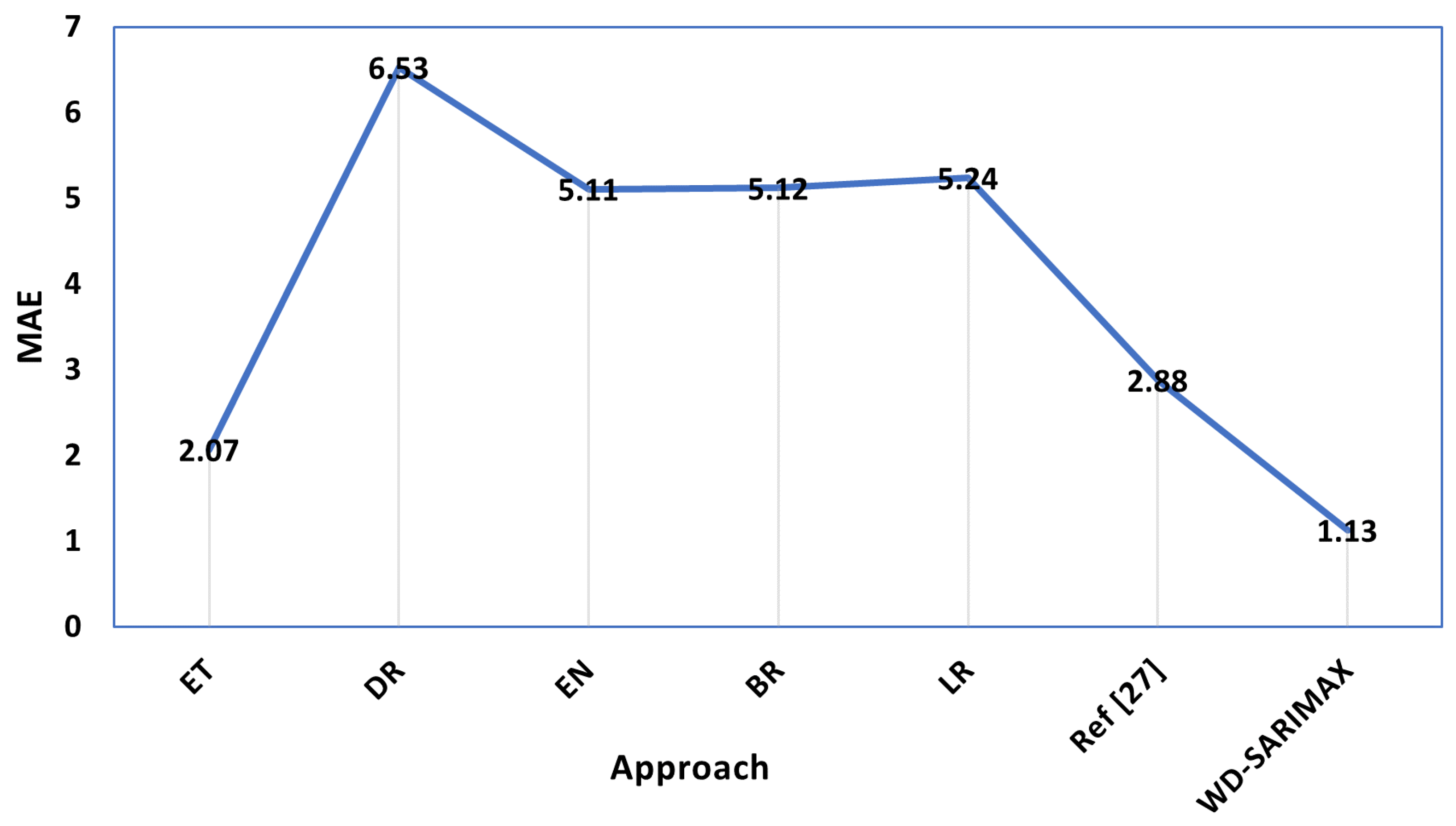
4.2. Evaluation Measures

The proposed WD-SARIMAX model is evaluated using the following metrics described in

Table 2. Statistical analysis for the features.

Metric	Value
MSE	$\frac{1}{O}{\sum }_{i=1}^O({\widehat{pred}}_i-Actua{l}_i{)}^2$	(19)
MAE	$\frac{1}{O}{\sum }_{i=1}^O|{\widehat{pred}}_i-Actua{l}_i|$	(20)
MedAE	$median(|{\widehat{pred}}_1-Actua{l}_1|,\dots ,|{\widehat{pred}}_i-Actua{l}_i|)$	(21)
RMSE	$\sqrt{\frac{1}{O}{\sum }_{i=1}^O({\widehat{pred}}_i-Actua{l}_i{)}^2}$	(22)
MAPE	$\left(\frac{1}{O}{\sum }_{i=1}^N\left|\frac{{\widehat{pred}}_i-Actua{l}_i}{Actua{l}_i}\right|\right)\times 100$	(23)
$R^2$	$1-\frac{{\sum }_{i=1}^O{(Actua{l}_i-{\widehat{pred}}_i)}^2}{{\sum }_{i=1}^O{\left(\left({\sum }_{i=1}^{O}Actua{l}_i\right)-Actua{l}_i\right)}^2}$	(24)

. This system of measurement includes Mean Square Error (MSE), Mean Absolute Error (MAE), Median Absolute Error (MedAE), Root Mean Square Error (RMSE), and Mean Absolute Percentage Error (MAPE). The coefficient of determination ($R^2$) where O is the number of observations in the dataset; ${\widehat{pred}}_i$ and $Actua{l}_i$ are the ith predicted and actual values and ${\overline{\widehat{pred}}}_i$ and ${\overline{Actual}}_{in}$ are the means of the predicted and actual values equations as shown in Equations (19)–(24).

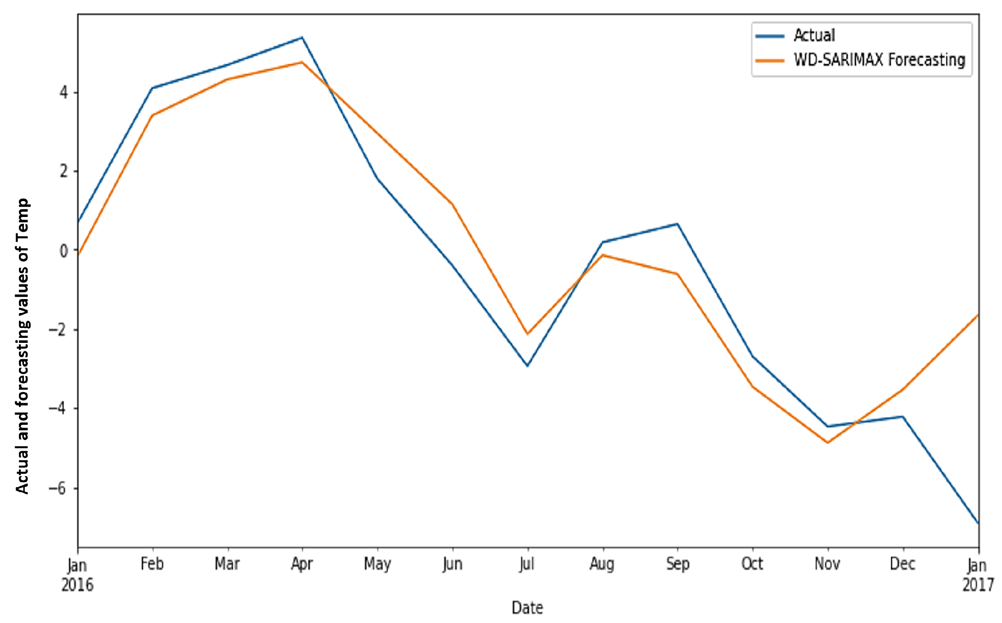
4.3. Results Analysis and Discussion

The experiment results were executed and written in Python 3.8 using the jupyter notebook version (6.4.6) with Intel Core i5 and 16 GB RAM using Microsoft Windows 10 x64-bit. Jupyter notebook helps write python codes, whereas Jupiter notebook is an open source utilized for constructing and executing several machine-learning models for classification and regression. Five machine learning (ML) regression models are used To evaluate the performance of the WD-SARIMAX model in wind power forecasting more effectively for comparison in the paper. The ML regression models are the Extra Trees (ET) regressor, Dummy Regressor (DR), Elastic Net (EN) regressor, Bayesian Ridge (BR) regressor, and Lasso Regressor (LR). In addition, Mean Squared Error (MSE), Mean Absolute Error (MAE), Median Absolute Error (MedAE), Root Mean Squared Error (RMSE), Mean Absolute Percentage Error (MAPE), and Coefficient of Determination ($R^2$) are used as evaluation metrics in this study.

Table 3. Specification of the parameter for the regression machine learning models.

Models	Parameters
ET	N_estimators = 10, criterion = squared${}_{e}rror$
DR	Strategy = mean
EN	Alpha = 0.1, fit_intercept = true
BR	N_iter = 200, fit_intercept = true
LR	Alpha = 0.01

illustrates the configuration of the parameters for regression models, ET, DR, EN, BR, and LR, used in this study to compare with the WD-SARIMAX model.

The experimental results of MSE, MAE, MedAE, RMSE, MAPE, and $R^2$ for the models, namely, WD-SARIMAX, ET, DR, EN, BR, and LR, respectively, are demonstrated in

Table 4. Comparison between the proposed WD-SARIMAX model and various ML regression models.

Models	MSE	MAE	MedAE	RMSE	MAPE	${\mathit{R}}^2$
ET	7.6	2.07	1.45	2.76	10.49	0.86
DR	66	6.53	5.37	8.12	37.3	0.21
EN	36.78	5.11	4.95	6.06	25.7	0.364
BR	36.83	5.12	4.97	6.08	25.9	0.36
LR	37.5	5.24	5	6.12	26.5	0.35
WD-SARIMAX	2.8	1.13	0.76	1.67	4.9	0.91

.

Among all the experimental models in Table 3, the WD-SARIMAX model gives the best results; its MSE, MAE, MedAE, RMSE, MAPE, and $R^2$ are 2.8, 1.13, 0.76, 1.67, 4.9, and 0.91, respectively. DR model gives the worst results; its MSE, MAE, MedAE, RMSE, MAPE, and $R^2$ are 66, 6.53, 5.37, 8.12, 37.3, and 0.21, respectively. For the ET model, the MSE, MAE, MedAE, RMSE, MAPE, and $R^2$ are 7.6, 2.07, 1.45, 2.76, 10.49, and 0.86, respectively. For the EN model, the MSE, MAE, MedAE, RMSE, MAPE, and $R^2$ are 36.78, 5.11, 4.95, 6.06, 25.7, and 0.364. For the BR model, the MSE, MAE, MedAE, RMSE, MAPE, and $R^2$ are 36.83, 5.12, 4.97, 6.08, 25.9, and 0.36, respectively. The MSE, MAE, MedAE, RMSE, MAPE, and $R^2$ for the LR model are 37.5, 5.24, 5, 6.12, 26.5, and 0.35, respectively.

Because the p-value is significantly higher than the significance level of 0.05, which is 0.45, indicating that the series is non-stationary. Therefore, Wavelet Decomposition (WD) is applied to make the series stationary by adapting the p-value to 0.05. Figure 5 demonstrates the time series plot for the temperature after using WD. The order of the SARIMAX model is calculated using (P, D, Q) (P, D, [Q], M) Order, where P represents the autoregressive order, D represents the integration order, Q represents the moving average order, and M represents the periodicity. P can be determined from the plot of Partial Autocorrelation (PACF) in Figure 6 in the research. PACF is determined as the correlation between the series and its lag after the contributions from intermediate lags are excluded. As seen in the PACF graph in Figure 6, the maximum lag with a value out of the confidence interval that is light blue is 4; thus, P is set to 4. D is set to 0 because the data time series is stationary. Q order can is calculated from the plot of Autocorrelation (ACF) in Figure 6. Autocorrelation is determined as the correlation of a single time series and a lagged copy of itself. As seen in the ACF graph in Figure 6, the maximum lag with a value out of the confidence interval that is light blue is 1; thus, Q is set to 1. M order presents the number of periods in the season that is 12 for monthly data; thus, M is set to 12. The autocorrelation between a time series analysis of temperature after resampling and the lag of ACF and PACF begins with a lag of 0, which is the time series’ correlation and yields a correlation of 1. In this paper, we come across 16 lags to investigate the ACF and PACF for the temperature after applying to resample, as shown in Figure 6.

Figure 7 illustrates the time series plot for the temperature after applying it to resample. Figure 8 demonstrates the actual and forecasted values for the WD-SARIMAX model. In Figure 8, the horizontal bar represents the time series analysis from January 2016 to January 2017, while the vertical bar represents the scaled temperature after applying WD.

The current efforts of the applied dataset demonstrated that the study is in between the period from 2013 to 2017. The main target of this work is to forecast the temperature effect on climate change through the next eight years until 2025. Therefore, Figure 9 shows the forecasting for the temperature in the next eight years. This study attempts to forecast the temperature in the next few years till 2025. As seen in Figure 9, the temperature will decrease slightly in the next eight years. During the period from 2018 to 2025, very slight changes took place, but there will be stability in temperatures, as shown in Figure 9 in this period. Most of the previous research studied changes for one year only, but in this research, the temperature was studied for the next eight years. For comparative analysis, in [27], they utilized the same dataset with Vector Auto Regressor (VAR) algorithm, and they achieved MAE 2.88 for the mean temperature, and 13.13, 1.92, and 27.45 for the humidity, wind speed, and mean pressure, respectively. This study uses the most recent dataset that includes temperature, humidity, wind speed, and mean pressure. Therefore, to our best knowledge, there is not much-related work concerned with the same dataset. Hence, we used ML approaches ET, DR, EN, BR, and LR compared with the proposed WD-SARIMAX to boot the obtained results and to make the proposed work more reliable in terms of MSE, MAE, MedAE, RMSE, and $R^2$. Figure 10 shows the comparative study of the proposed WD-SARIMAX with ML models and [27] based on determining the MAE.

5. Conclusions

In this study, a practical model called Wavelet Decomposition-Seasonal Auto-Regressive Integrated Moving Average with Exogenous Variables (WD-SARIMAX) is constructed for forecasting the temperature in Delhi city. Different evaluation metrics, namely, MSE, MAE, MedAE, RMSE, MAPE, and $R^2$, were used to evaluate the impact of the WD-SARIMAX model. The MSE, MAE, MedAE, RMSE, MAPE, and $R^2$ for the WD-SARIMAX model are 2.80, 1.13, 0.76, 1.67, 4.90, and 0.91, respectively. We further forecast the temperature progress during the period from 2017 to 2025 to study the effect of the temperature on climate change in the next few years. The proposed WD-SARIMAX model was compared with other machine learning regression models, where the WD-SARIMAX model achieved the best results. The worst results were obtained by the DR model; its MSE, MAE, MedAE, RMSE, MAPE, and $R^2$ are 66.00, 6.53, 5.37, 8.12, 37.30, and 0.21, respectively. In the future, new metaheuristic models [28,29,30,31] will be applied to this dataset to acquire better results.

References

1. Pachauri, R.K.; Reisinger, A. Climate Change 2007. Synthesis Report. Contribution of Working Groups I, II and III to the Fourth Assessment Report; IPCC: Geneva, Switzerland, 2008; Volume 1, pp. 1–103.
2. Maray, M.; Alghamdi, M.; Alrayes, F.S.; Alotaibi, S.S.; Alazwari, S.; Alabdan, R.; Al Duhayyim, M. Intelligent metaheuristics with optimal machine learning approach for malware detection on IoT-enabled maritime transportation systems. Expert Syst. 2022, 39, e13155. [Google Scholar] [CrossRef]
3. Shaiba, H.; Marzouk, R.; Nour, M.K.; Negm, N.; Hilal, A.M.; Mohamed, A.; Motwakel, A.; Yaseen, I.; Zamani, A.S.; Rizwanullah, M.; et al. Weather forecasting prediction using ensemble machine learning for big data applications. Comput. Mater. Contin. 2022, 73, 3367–3382. [Google Scholar] [CrossRef]
4. Bartos, I.; Jánosi, I.M. Nonlinear correlations of daily temperature records over land. Nonlinear Process. Geophys. 2006, 13, 571–576. [Google Scholar] [CrossRef] [Green Version]
5. Bonsal, B.R.; Zhang, X.; Vincent, L.A.; Hogg, W.D. Characteristics of daily and extreme temperatures over Canada. J. Clim. 2001, 14, 1959–1976. [Google Scholar] [CrossRef]
6. Mengash, H.A.; Hussain, L.; Mahgoub, H.; Al-Qarafi, A.; Nour, M.K.; Marzouk, R.; Qureshi, S.A.; Hilal, A.M. Smart cities-based improving atmospheric particulate matters prediction using chi-square feature selection methods by employing machine learning techniques. Appl. Artif. Intell. 2022, 36, 2067647. [Google Scholar] [CrossRef]
7. Alhakami, H.; Kamal, M.; Sulaiman, M.; Alhakami, W.; Baz, A. A Machine Learning Strategy for the Quantitative Analysis of the Global Warming Impact on Marine Ecosystems. Symmetry 2022, 14, 2023. [Google Scholar] [CrossRef]
8. Kim, S.; Lee, P.-Y.; Lee, M.; Kim, J.; Na, W. Improved State-of-health prediction based on auto-regressive integrated moving average with exogenous variables model in overcoming battery degradation-dependent internal parameter variation. J. Energy Storage 2022, 46, 103888. [Google Scholar] [CrossRef]
9. Cifuentes, J.; Marulanda, G.; Bello, A.; Reneses, J. Air temperature forecasting using machine learning techniques: A review. Energies 2020, 13, 4215. [Google Scholar] [CrossRef]
10. Oo, Z.Z.; Sabai, P. Time Series Prediction Based on Facebook Prophet: A Case Study, Temperature Forecasting in Myintkyina. Int. J. Appl. Math. Electron. Comput. 2020, 8, 263–267. [Google Scholar] [CrossRef]
11. Liu, N.; Babushkin, V.; Afshari, A. Short-term forecasting of temperature driven electricity load using time series and neural network model. J. Clean Energy Technol. 2014, 2, 327–331. [Google Scholar] [CrossRef]
12. Zhang, H.; Wang, Y.; Chen, D.; Feng, D.; You, X.; Wu, W. Temperature Forecasting Correction Based on Operational GRAPES-3km Model Using Machine Learning Methods. Atmosphere 2022, 13, 362. [Google Scholar] [CrossRef]
13. Zhang, Z.; Dong, Y. Temperature forecasting via convolutional recurrent neural networks based on time-series data. Complexity 2020, 2020, 3536572. [Google Scholar] [CrossRef]
14. Nandi, A.; De, A.; Mallick, A.; Middya, A.I.; Roy, S. Attention based long-term air temperature forecasting network: ALTF Net. Knowl.-Based Syst. 2022, 252, 109442. [Google Scholar] [CrossRef]
15. Ajewole, K.P.; Adejuwon, S.O.; Jemilohun, V.G. Test for stationarity on inflation rates in Nigeria using augmented dickey fuller test and Phillips-persons test. J. Math. 2020, 16, 11–14. [Google Scholar]
16. Zhang, S.; Monekosso, D.; Remagnino, P. Data pre-processing and model selection strategies for human posture recognition. In Proceedings of the 2018 11th International Symposium on Communication Systems, Networks Digital Signal Processing (CSNDSP), Budapest, Hungary, 18–20 July 2018; pp. 1–6. [Google Scholar]
17. Rhif, M.; Abbes, A.B.; Farah, I.R.; Martínez, B.; Sang, Y. Wavelet transform application for/in non-stationary time-series analysis: A review. Appl. Sci. 2019, 9, 1345. [Google Scholar] [CrossRef] [Green Version]
18. Paul, R.K.; Paul, A.K.; Bhar, L.M. Wavelet-based combination approach for modeling sub-divisional rainfall in India. Theor. Appl. Climatol. 2020, 139, 949–963. [Google Scholar] [CrossRef]
19. Peng, M.; Zhang, Q.; Xing, X.; Gui, T.; Huang, X.; Jiang, Y.G.; Ding, K.; Chen, Z. Trainable undersampling for class-imbalance learning. Proc. AAAI Conf. Artif. Intell. 2019, 33, 4707–4714. [Google Scholar] [CrossRef] [Green Version]
20. Kim, K.-R.; Park, J.-E.; Jang, I.-T. Outpatient forecasting model in spine hospital using ARIMA and SARIMA methods. J. Hosp. Manag. Health Policy 2020, 2020, 1–8. [Google Scholar] [CrossRef]
21. Tiwari, D.; Bhati, B.S. A deep analysis and prediction of covid-19 in India: Using ensemble regression approach. In Artificial Intelligence and Machine Learning for COVID-19; Springer: Berlin/Heidelberg, Germany, 2021; pp. 97–109. [Google Scholar]
22. Trenchevski, A.; Kalendar, M.; Gjoreski, H.; Efnusheva, D. Prediction of air pollution concentration using weather data and regression models. Proc. Int. Conf. Appl. Innov. IT 2020, 8, 55–61. [Google Scholar]
23. Mardhiyyah, Y.S.; Rasyidi, M.A.; Hidayah, L. Factors affecting crowdfunding investor number in agricultural projects: The dummy regression model. J. Manaj. Agribisnis 2020, 17, 14. [Google Scholar] [CrossRef]
24. Saqib, M. Forecasting COVID-19 outbreak progression using hybrid polynomial-Bayesian ridge regression model. Appl. Intell. 2021, 51, 2703–2713. [Google Scholar] [CrossRef] [PubMed]
25. Ranstam, J.; Cook, J.A. LASSO regression. J. Br. Surg. 2018, 105, 1348. [Google Scholar] [CrossRef]
26. Johnsen, T.K.; Gao, J.Z. Elastic net to forecast COVID-19 cases. In Proceedings of the 2020 International Conference on Innovation and Intelligence for Informatics, Computing and Technologies (3ICT), Sakhir, Bahrain, 20–21 December 2020; pp. 1–6. [Google Scholar]
27. Antonicelli, M.; Maggino, F. Big data and official statistics: General Concepts and Statistical Instruments. In Big Data and Official Statistics, 1st ed.; Egea editor: Milano, Italy, 2022; Volume 2022, pp. 160–168. [Google Scholar]
28. Nagappan, K.; Rajendran, S.; Alotaibi, Y. Trust Aware Multi-Objective Metaheuristic Optimization Based Secure Route Planning Technique for Cluster Based IIoT Environment. IEEE Access 2022, 10, 112686–112694. [Google Scholar] [CrossRef]
29. El-Kenawy, E.-S.M.; Mirjalili, S.; Alassery, F.; Zhang, Y.; Eid, M.M.; El-Mashad, S.Y.; Aloyaydi, B.A.; Ibrahim, A.; Abdelhamid, A.A. Novel meta-heuristic algorithm for feature selection, unconstrained functions and engineering problems. IEEE Access 2022, 10, 40536–40555. [Google Scholar] [CrossRef]
30. Abdelhamid, A.; El-kenawy, E.-S.M.; Alotaibi, B.; Abdelkader, M.; Ibrahim, A.; Eid, M.M. Robust speech emotion recognition using CNN+LSTM based on stochastic fractal search optimization algorithm. IEEE Access 2022, 10, 49265–49284. [Google Scholar] [CrossRef]
31. Khafaga, D.; Alhussan, A.; El-Kenawy, E.-S.M.; Ibrahim, A.; Eid, M.M.; Abdelhamid, A. Solving optimization problems of metamaterial and double T-shape antennas using advanced meta-heuristics algorithms. IEEE Access 2022, 10, 74449–74471. [Google Scholar] [CrossRef]
Figure 1. Proposed methodology and process for the WD-SARIMAX model.
Sustainability 15 00757 g001
Figure 2. Time series plot for the original data.
Sustainability 15 00757 g002
Figure 3. Histogram visualization for the features.
Sustainability 15 00757 g003
Figure 4. Metrics for evaluating the performance of the proposed method.
Sustainability 15 00757 g004
Figure 5. Time series plot for the temperature after applying WD.
Sustainability 15 00757 g005
Figure 6. ACF and PACF for the temperature after resampling.
Sustainability 15 00757 g006
Figure 7. Time series plot for the temperature after resampling.
Sustainability 15 00757 g007
Figure 8. Actual values and Forecasting values based on WD-SARIMAX.
Sustainability 15 00757 g008
Figure 9. Forecasting for the temperature in the next eight years.
Sustainability 15 00757 g009
Figure 10. The MAE of the proposed WD-SARIMAX compared with the ML models and [27].
Sustainability 15 00757 g010