Short-Term Traffic Congestion Prediction Using Hybrid Deep Learning Technique

Abstract

A vital problem faced by urban areas, traffic congestion impacts wealth, climate, and air pollution in cities. Sustainable transportation systems (STSs) play a crucial role in traffic congestion prediction for adopting transportation networks to improve the efficiency and capacity of traffic management. In STSs, one of the essential functional areas is the advanced traffic management system, which alleviates traffic congestion by locating traffic bottlenecks to intensify the interpretation of the traffic network. Furthermore, in urban areas, accurate short-term traffic congestion forecasting is critical for designing transport infrastructure and for the real-time optimization of traffic. The main objective of this paper was to devise a method to predict short-term traffic congestion (STTC) every 5 min over 1 h. This paper proposes a hybrid Xception support vector machine (XPSVM) classifier model to predict STTC. Primarily, the Xception classifier uses separable convolution, ReLU, and convolution techniques to predict the feature detection in the dataset. Secondarily, the support vector machine (SVM) classifier operates maximum marginal separations to predict the output more accurately using the weight regularization technique and a fine-tuned binary hyperplane mechanism. The dataset used in this work was taken from Google Maps and comprised snapshots of Bangalore, Karnataka, taken using the Selenium automation tool. The experimental outcome showed that the proposed model forecasted traffic congestion with an accuracy of 97.16%.

1. Introduction

Traffic congestion in metropolitan areas has gradually grown over the years to be one of the significant challenges for urban populations. Time-wasting and pollution are among the problems caused by motor traffic congestion, for which various solutions have been proposed, from toll regulation to minimum numbers of automobiles allowed to drive. Conventional STSs only partially address and overcome precision, instantaneity, and scalability concerns when dealing with traffic congestion in Internet of Vehicles (IoV) ecosystems. At present, heavy traffic in metropolitan areas is a universal problem that can lead to a variety of concerns, such as reduced traffic efficiency, rising traffic fatalities, etc. Road congestion estimation has become progressively important in STSs, since it plays a crucial task in route guidance and traffic management [1]. Urban areas have experienced a significant increase in traffic congestion over the past several decades. Traffic congestion not only adversely influences people’s lives, but also restricts reliable social and economic advancement. In addition, traffic congestion increases air pollution, journey times, and economic disruption. Traffic management methods are continuously developed in the attempt to track and evaluate traffic congestion. However, finding a solution remains challenging due to the problem’s complexity; specifically, traffic congestion is hard to forecast. The continuous and interconnected elements of traffic congestion illustrate its diverse nature and its ability to spread from one crowded road segment to another. Due to these difficulties, the assessment of traffic congestion is a challenging task. Adaptive ride sharing minimizes the volume of traffic. A flexible ride-sharing service can vastly improve traffic conditions when inflation is high, particularly during peak hours. Sharing can diminish the long, multi mile journeys associated with operating a mobility service; however, the scenario is vastly different when ride sharing is confined to small- and medium-sized areas. Furthermore, a fine-tuned ride sharing system relies upon the accurate forecasting of the needs in the near future. The explanation is that mobility services vastly increase the total trip length, and pooling is merely a way to counter this pattern rather than eradicating congestion when trip density is insufficient [2].

Numerous studies have attempted to solve traffic congestion prediction using vehicular adhoc network technology (VANET) [3]. However, theoretically, road congestion likely diminishes with the increase in the costs of transport infrastructure or the implementation of effective traffic techniques, including short-term traffic forecasting or the study of congestion patterns, which can be effectively applied to existing road networks at a low cost. Due to the paucity of data, the initial prediction generally concentrates on traffic metrics such as velocity, quantity, and traffic flow in a section of a roadway, or a collection of streets, or modest roadways [4]. There needs to be more initiatives aimed at forecasting road network status to avoid undesirable situations for travelers and traffic authorities. The scientific literature utilizes information retrieved using either connections of moving automobiles (e.g., VANET and floating cars) running on each path or static devices (e.g., detectors, inductive loops, traffic cameras, etc.) located across all routes. Recently, web apps such as Google Traffic began to publicly offer reliable real-time traffic data for all cities, including the congestion level and the road section’s average speed. As a result of more numerous motorized vehicles, urbanism, and the growing population, especially in metropolitan areas, congestion instances have increased globally. Congestion increases travel time, poor air quality, and fuel costs while decreasing the usage of the transport system, which might result in the deterioration of social, ecological, and global systems. Roadblocks cause the majority of congestion instances; the advanced traffic management (ATM) system in STSs seeks to identify these roadblocks and take necessary measures to relieve bottlenecks and enhance the effectiveness of the transit system [5]. Road traffic congestion (RTCs) is a significant worldwide issue; when there is an increase in the demand for transit operations above the capacity of the system, unexpected capacity constraints (RTC) arise. Traffic congestion costs the South African Rand (ZAR) economy billions of each year. On a worldwide basis, cities such as Bengaluru, India, are among the most affected by this issue. The top five most congested cities in the world are Istanbul (Turkey), Moscow (Russia), Kyiv (Ukraine), Bogota (Colombia), and Mumbai (India). Escalating traffic congestion is the direct and indirect consequence of a significant portion of road traffic collisions, leading to increasing number of accidents and mortality rates on highways worldwide [6]. The World Health Organization (WHO) confirmed that RTC causes health problems that lead to about 3.7 million deaths around the world, especially in developing cities, where money losses, delays, fuel waste, road accidents, and pollution are significant. In addition, sulfur oxide, carbon monoxide, and nitrogen oxide are produced. Moreover, according to the report, the primary pollutants in the air are connected to road traffic congestion, which causes ailments affecting the cardiovascular system. Congested roads pose a threat to those stuck in congestion, as well as residents who live in close proximity to motorways [7]. In this research paper, an algorithm for forecasting gridlock on highways with supervised hybrid approaches is proposed. In deep learning, hybrid techniques enhance several classifiers and improve their effectiveness. As a result, hybrid methods have demonstrated superior efficiency in road traffic congestion applications [8].

The primary contributions of the paper are as follows:

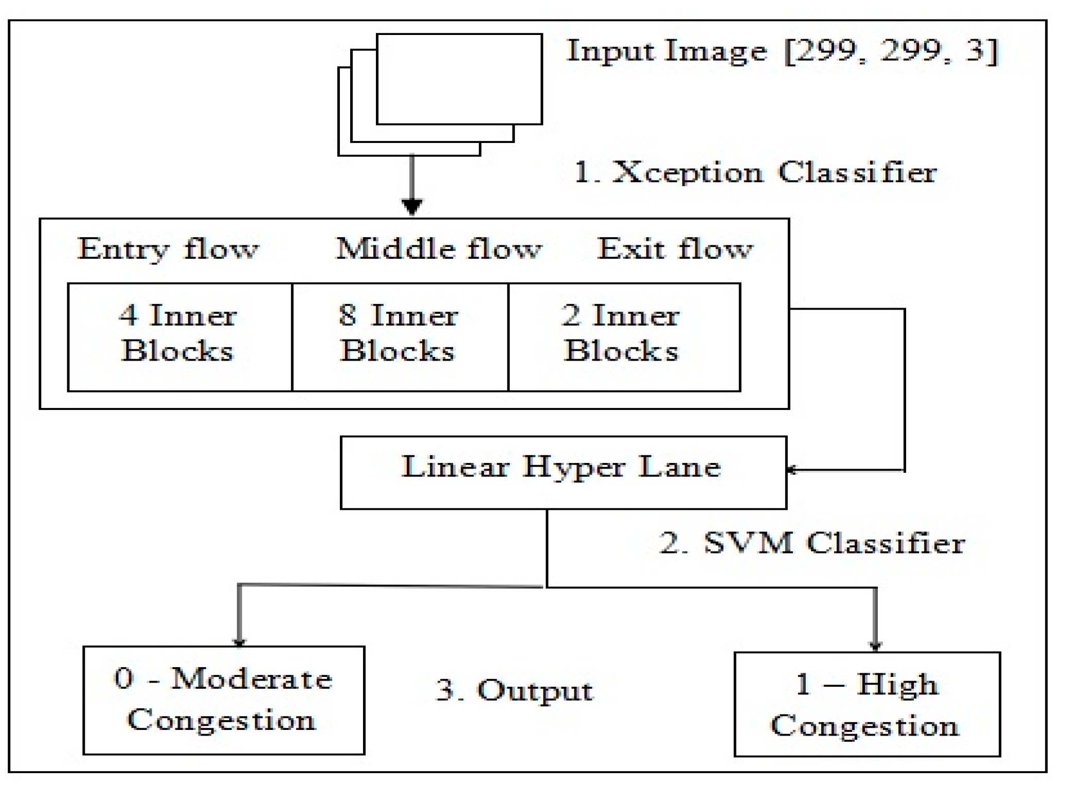
• We proposed a hybrid Xception—support vector machine (XPSVM) classifier model to predict STTC every 5 min over 1 h.
• We propose the Xception classifier, which uses separable convolution, ReLU, and convolution techniques to predict feature congestion based on a traffic dataset.
• We propose an SVM classifier that uses maximum marginal separations to predict the output in a more accurate way using the weight regularization technique. We conducted in-depth tests using urban road congestion data to explore the reliability of the proposed model.

The rest of the paper is organized as follows: The literature review is presented in Section 2. The materials and methods of the proposed XPSVM framework are discussed in Section 3. Section 4 addresses the implementation. The results of the experiments used to validate the proposed methodology and their analysis are presented in Section 5. The conclusion and directions for future work are presented in Section 6.

2. Literature Review

STSs and current transport policies have heavily relied on short-term traffic predictions since the 1970s. Estimating traffic congestion instances is mostly based on assumptions about short-term traffic flow prediction. Techniques for predicting the volume of traffic can be grouped into three categories: parametric-, non-parametric-, and knowledge-based techniques [9]. The autoregressive integrated moving average (ARIMA) framework was initially proposed to build a model using historical time series to forecast future principles. The Box–Jenkins technique was used to customize the ARIMA model parameters. Smith and Williams used the ARIMA model to forecast the traffic flow at a specific point in time given the initial moment. Furthermore, seasonal ARIMA (SARIMA) methods were discovered to have significant computational complexity [10]. Many researchers have investigated deep learning because it seems to be an effective way to find patterns in data. Deep learning has been used in many different fields because of its significant ability to make predictions. Sukode S et al. [11] primarily used floating car data, i.e., information about global positioning system (GPS)-equipped motors obtained using sensing devices for restriction, such as wire loops, video recorders, and infrared mechanics. The transport system model limits flexibility, even though it is the most popular model and has excellent reliability and accurate systematization. Gramaglia M et al. [12] leveraged vehicle-to-vehicle (V2V) devices to collect automobile road information, consolidating transit model properties such as speed, density, flow, and journey time. Wen F et al. [13] proposed a technique called Hybrid Temporal Association Rules Mining, which uses the density-based spatial clustering of applications with noise (DBSCAN) and is employed to identify traffic conditions and produce guidelines for forecasting road congestion in the transport network. Ranjan N et al. [14] proposed a hybrid model that effectively learns the spatio-temporal relationships among pieces of information by merging a convolutional neural network, long short-term memory (LSTM), and a transposed convolutional network. Tseng F H et al. [15] proposed an SVM-based actual highway traffic congestion prediction (SRHTCP) algorithm that gathers highway information from Taiwan’s Area National Freeway Bureau, i.e., data of road incidents observed by motorists (obtained from Taiwan’s Police Broadcasting Service) and meteorological data (obtained from Taiwan’s Central Weather Bureau). The fuzzy theory estimates the congestion of an elevated highway stretch in real time, considering road velocity, road density, and rainfall. Zhang S et al. [16] proposed a simple and broad workflow for collecting massive road congestion data and creating datasets using image processing. The Washington State Department of Transportation utilizes screenshots of the road congestion navigation performed by web traffic providers to create a status report called Seattle area traffic congestion status (SATCS). Synchronous layers in the encoder and decoder of a deep auto-encoder neural network model are used to find temporal correlations between transport systems and forecasted road bottlenecks. Chakraborty P et al. [17] presented deep learning methods, the conventional deep convolutional neural network (DCNN), and you only look once (YOLO) methods to recognize traffic jams in camera photos. In their study, the shallow technique of support vector machine (SVM) was deployed as a benchmark to evaluate the advantages of deep learning models. Traffic congestion visuals in the dataset were labeled, and the models were trained using square footage data of adjacent sensor devices. Nagy A. M et al. [18] launched a novel traffic forecasting approach, the congestion-based traffic prediction model (CTPM), to demonstrate how using gridlock data can significantly enhance projection. This framework updates earlier predictions based on bottleneck patterns. There is no requirement to change effective procedures because the model output can be combined with any prior model. Elfar A et al. [19] evaluated the incorporation of floating car data accessible using smart transport systems along with logistic regression, random forests, and neural networks to anticipate STTC. In their study, transportation movements were analyzed with next generation simulation (NGSIM) software. In their analyses, two distinct analytics were developed: (1) offline models were trained using historical information and upgraded (re-trained) any time essential modification were necessary, including notifications to the architecture; (2) online models were trained using historical information and regularly updated utilizing actual data on current traffic patterns retrieved via V2V/vehicle-to-infrastructure (V2I) connectivity. Lee W H et al. [5] devised a three-phase spatio-temporal traffic bottleneck mining (STBM) approach that combines several traffic patterns. The STBM techniques employ raw information to identify urban system spatio-temporal traffic bottlenecks using location-based utility. The STBM prototype system was based on the taxi dispatching system used in the metropolitan network of Taipei, Taiwan. Li Tao et al. [20] presented the convolutional neural network bidirectional long short-term memory (Conv-BiLSTM) technique, which incorporates CNN and BiLSTM with spatio-temporal characteristics. Initially, the retrieved speed of traffic information is compressed thanks to the spatio-temporal capabilities, and a three-dimensional matrix is built for the forecasting system. Then, the CNN includes the spatial features, and BiLSTM retrieves the temporal characteristics; finally, the forecasting results are generated as a throughput. Meng Chen et al. [21] proposed a novel approach, the pulse-coupled neural network (PCNN), developed based on deep convolutional neural networks with two essential methods: time-series folding and multi-grained learning. First, the time series is folded to compensate for adequate traffic conditions and historical traffic patterns. Next, a 2-D matrix is built as the input data, using a series of convolutions over the input sequence. This approach can simulate regional and temporal dependency, and multiscale traffic conditions. Xiaolei Ma et al. [22] aimed to apply deep learning models to investigate transport systems comprehensively. They relied on car GPS data, a deep restricted Boltzmann machine (RBM), and a recurrent neural network (RNN). The RNN-RBM framework was then employed to analyze the expansion of traffic congestion. A statistical study was conducted in Ningbo, China, to authenticate the efficiency of the suggested method. Jinchao Song et al. [23] focused on locating spatio-temporal patterns and predicting potential motorists incurring in road congestion. The k-means clustering method was used to identify the spatio-temporal dissemination of busy routes utilizing actual traffic information obtained from an online resource. Finally, they used a geographical detector (Geo-detector) to extract the possible elements with both spatio-temporal sequences. During weekdays, the consequences revealed six congestion trends on intra-regional and inter-regional roadways. M. Gollapalli et al. [24] proposed a cloud-based intelligent road traffic congestion prediction model powered by a hybrid neuro-fuzzy method to decrease vehicle delays at various road junctions. The proposed model aims to assist automated traffic management systems in lessening congestion, especially in smart cities where IoT sensors are deployed along the route. Liu L et al. [25] devised a traffic congestion situation assessments (TCSA) strategy for a fuzzy integrated multi-metric assessment based on three predicted vehicle traffic variables aimed at the 5G Internet of Vehicles setting. The smoothing coefficient and model weight may be adjusted with the prediction algorithm. The trapezoidal membership function is used to calculate the traffic congestion index membership degree, and the adaptive critic method is used to calculate traffic congestion evaluation metrics weights. Finally, Bokaba T et al. [26] used data collected from a roadway in Gauteng Province, South Africa, to determine vehicle traffic flow in advance. In general, ensemble learning can improve the performance of weak classifiers. In this study, to compare the predictive performance of the proposed methods, a real-world dataset was used, as well as bagging, boosting, stacking, and random forest ensemble models. The ensemble prediction model was designed to forecast traffic congestion on roads.

3. Materials and Methods

3.1. XPSVM Method

In this section, we present the construction of an XPSVM method to analyze STTC. The XPSVM method is designed to predict STTC every 5 min over 1 h, which could help to reduce travel costs, travel time, air pollution, and global warming. The following subsections provide additional information about the proposed XPSVM architecture. Figure 1 depicts the proposed XPSVM architecture.

3.2. Xception Classifier

Francois Chollet introduced Xception Model. Xception is an Inception Architecture augmentation that replaces standard Inception modules with depthwise separable convolutions. The Xception technique is an improved variant of the Inception model used in convolutional neural networks (CNNs). This model has deep convolution layers and wider convolution layers that operate simultaneously. This model offers a 71-layer deep CNN, which was developed based on an extreme version of the Inception model and was prompted by Google. This framework is layered with depthwise separable convolution layers. The pre-trained variant of the method is trained to use millions of pictures from the Imagenet database. Furthermore, this method provides comprehensive representations of its utility for a wide variety of images and can identify hundreds of different classifiers. The Xception method is extremely useful in image recognition and classification. In this design, the input is sent via the entry flow, middle flow, and exit flow. Further batch normalization considers all convolution and separable convolution layers. The Xception architecture is formed by 36 convolution layers, which are the core of the network used for extracting features. A dense layer accompanies the convolutional basis because the model strategies focus on image categorization. In addition to the initial and final components, all 14 components, composed of 36 convolution layers, have linear residual connections enclosing themselves. A structure provided by Xception is composed of depthwise separable convolution blocks and Maxpooling, all of which are connected via shortcuts similar to their use in residual neural network (ResNet) variants. The Xception framework is a linear stack of residually connected depthwise separable convolution layers. An effective Xception framework depends on two fundamental ideas: 1. depthwise separable convolution, and 2. convolution blocks shortcuts that are similar to ResNet. Depthwise separable convolutions are alternatives to traditional convolutions and are reported to be substantially more efficient in terms of computing time [27]. Figure 2 below illustrates the Xception classifier.

3.3. Support Vector Machine Classifier

SVM is a type of supervised machine learning that tries to find a hyperplane in the N-dimensional space (where N is the number of features) that uniquely distinguishes sample units. Numerous hyperplanes can be employed to determine the uniting classes of two data points. The aim is to identify a plane containing the maximum distance between each group’s data points. Expanding the margin gap offers reinforcement, enabling additional data points to be labeled as preferable confidence. Figure 3 depicts the SVM classifier.

In SVM, we can encounter two cases, namely, linearly separable and non-linearly separable cases. In the linearly separable case, we utilize linear SVM only when the data are linearly separable. Perfectly linearly separable data points can be divided into two classes using a single straight line (if in 2D). In the non-linearly separable case, SVM can be used to classify data when they cannot be categorized into two parts using a straight line (2D), which necessitates the employment of more sophisticated approaches, such as the kernel trick. We do not encounter linearly separable data points throughout many real-world scenarios; thus, we apply the kernel method to solve them. The Kernel trick uses existing attributes to seek a few transformations and develop new features. These new attributes are significant for SVM in determining the nonlinear decision boundary. Support vectors are the nearest points to the hyperplane those data points are employed as separate lines. The margin is the separation between the hyperplane and the closest observations to the hyperplane (support vectors). Large margins are regarded as acceptable margins in SVM. Below is an example of a hyperplane’s equation (Equation (1)):

$$c·y+d=0,$$

(1)

where

• c—is a vector normal to the hyperplane,
• y—is the input vector, and
• d—is the offset.

3.3.1. Dot Product in SVM

Dot product pertains to the projection of any vector on another vector. As a result, we extract the dot product of y vectors and x vectors. If the dot product is more significant than ‘a,’ as shown in Equation (2), then the point is on the right side; if the dot product is smaller than ‘a,’ as shown in Equation (3), the point is on the left side; if it is equal to ‘a,’ as shown in Equation (4), the point is on the decision boundary:

$$\overline{\mathrm{Y}}·\overline{\mathrm{x}}>\mathrm{a}, (\mathrm{positive} \mathrm{samples})$$

(2)

$$\overline{\mathrm{Y}}·\overline{\mathrm{x}}<\mathrm{a}, (\mathrm{negative} \mathrm{samples})$$

(3)

$$\overline{\mathrm{Y}}·\overline{\mathrm{x}}= \mathrm{a}, (\mathrm{point} \mathrm{lies} \mathrm{on} \mathrm{the} \mathrm{decision} \mathrm{boundary})$$

(4)

where

• $\overline{\mathrm{Y}}$—is a vector
• $\overline{\mathrm{x}}$—is a vector and
• a—is the decision boundary.

Although neural networks are excellent function approximators and feature extractors, they may overfit due to their weights being overly focused. In this situation, the theory of regularization is significant.

3.3.2. L2 Regularization

L2 regularization is a type of regularization method called parameter norm penalty. This technique performs the norm of a specific parameter; usually, weights are appended to the objective function to enhance the L2 norm, and an additional term known as the regularization term is introduced to the network’s cost function as shown in Equation (5). The following is the general formula for L2 regularization:

$$\mathrm{C}={\mathrm{C}}_0+\frac{\mathsf{\gamma }}{2\mathrm{n}}{\displaystyle \sum }_{\mathsf{\omega }}{\mathsf{\omega }}^2$$

(5)

where

• C—is the regularized cost function,
• C₀—is the unregularized cost function,
• γ—is the regularization parameter,
• n—is the number of features, and
• $\mathsf{\omega }$—is the weight.

3.3.3. Cost Function and Gradient Updates

Using the SVM classifier, we want to reduce the hyperplane distance among data points. Hinge loss is a loss function, as shown in Equation (6), that assists in margin optimization [28]. The hinge loss function is represented by the formula below:

$$\mathrm{C}\left(\mathrm{x},\mathrm{y},\mathrm{f}\left(\mathrm{x}\right)\right)=\{\begin{array}{c}0, \mathrm{i}\mathrm{f} \mathrm{y}\ast \mathrm{f}\left(\mathrm{x}\right)\ge 1\\ 1-\mathrm{y}\ast \mathrm{f}\left(\mathrm{x}\right), \mathrm{e}\mathrm{l}\mathrm{s}\mathrm{e} \end{array}$$

(6)

where

• C—is the cost function,
• x—is the input vector,
• y—is the true class, and
• f(x)—is the output of SVM given input x.

When the cost is zero, the projected and actual variables have the same sign. If the cost is not-zero, we compute the loss value. In addition, we add a regularization parameter to the cost function. The main goal of the regularization parameter is to balance margin maximization and loss.

4. Implementation

The XPSVM algorithm steps are depicted below in Algorithm 1.

Algorithm 1 Algorithm of XPSVM

(A) Xception: 1. Create imagedatagenerator to load image data from the train directory with batch size as 32 or 64, class mode as “categorial” and each image in 2D Array [299, 299]. 2. Similarly, create imagedatagenerator to load image data from test directory with batch size as 32 or 64, class mode as “categorial” and each image in 2D Array [299, 299]. 3. Create a sequential model with hidden layers as per the architecture of Xception or create the instance of in built trained Xception Model using keras (using this in-built model). 4. Disable already trained 14 blocks (layers) of Xception. 5. Pop out the default output layers of Xception model to add the custom output layers. 6. Add the fully connected (output) layers.    6.1 Add the flatten layer.    6.2. Add 3 dense layers with neuron as 200, 100, 50, and activation function as “relu”. NOTE: reason to choose only 3 dense. Sol: optimum number of output layers to the chosen image data is 3, which are tested using keras tuner frame work. (B) SVM: (Supervised Linear Regressor). 7. Add another dense layer with:    7.1 Neurons—2 because we have two classifications (moderate and high congestion).    7.2 Kernel regularizes—keras regularizes l2 with value as 0.001 (it can be customized, but 0.001 was giving best accuracy).    7.3 Activation functions—linear (reason: the problem statement is binary classification). 8. Compile the created XceptionSVM Model with:    8.1 Optimizer function—Adam    8.2 Loss function—categorical hinge (due to binary classification, we use loss function). 9. Train or fit the XceptionSVM model for 150 Epochs and capture the loss, accuracy values of each epoch of training, validation images.

In this study, we used the GridsearchCV hyperparameter tuner, as shown below in

Table 1. Hyperparameter settings.

Hyperparameter	Input Values	Best Parameter Values
Epochs	10, 15, 20, 25, 30, 35, 40	25
Hidden Layers	14, 28, 42	14
Neurons in hidden layer	10, 15, 20, 25, 30	10
Dense layers	3, 6, 9, 12, 15	3
1st dense layer neurons	200, 300, 400	200
2nd dense layer neurons	100, 200, 300	100
3rd dense layer neurons	50, 100, 150	50
Dense layers activation functions	relu, sigmoid, softmax, softplus, tanh, exponential	Relu
Kernel regularizer	L1,L2	L1
L2 regularizer weights	0.1, 0.01, 0.001	0.001
Loss functions	categorical hinge, categorical, categorical cross entropy	categorical hinge
Optimizer	adam, adadelta, sgd, adamax, nadam	Adam

.

The parameter configurations of the Xception classifier and SVM classifier are shown below in

Table 2. Xception Parameters.

Parameters	Values
Input Parameters	3D Array with Size as (299, 299, 3)
Epochs	25
Flatten layers	1
Separableconvolution layers	34
Convolution layers	6
Maxpooling layers	4
Dense layers (fully connected layer)	3
Neurons in each dense layer	200, 100, 50 Successively
Loss function	categorical hinge marginal loss function
Activation function	relu activation
Optimizer	Adam

and

Table 3. SVM Parameters.

Parameters	Values
Input parameters	3D array with size as (x, x, 50) where x is >=1
Output parameters	2 (high congestion and low congestion)
Epochs	25
Regularizer	L2 weight regularizer
Regularizer variable weight	0.01 to 0.001
Kernel function	linear because output variables are two
Marginal planes	two, one each for two output variables

, respectively.

The experimental platforms used for this research study are as follows:

• Hardware: i7 Processor, 16 GB RAM, Graphics processing unit (GPU).
• Software: macOS Catalina, Python 3.10.5, API-Keras.

5. Experiments and Results Analysis

5.1. Data Description

In this study, traffic congestion data were collected by taking a snapshot using the online service provider Google Maps with the Selenium tool. The traffic images collected during the morning and evening peak hours were around 2500. The dataset contained factors such as parking, loading, unloading, two-wheel, and public transport vehicles on rainy, snowy, heavily windy, and sunny days at peak and off-peak times near major and minor traffic signal junctions during public and non-public holidays. In addition, small slippery roads were considered. The traffic images were taken from ITI Bus Depot, K R Puram, Bengaluru, Karnataka, India, to Halsuru Traffic police station, Bengaluru, Karnataka, India. We tested the effectiveness of the XPSVM model using real datasets of traffic congestion data obtained over the period from 11 May 2022 to 13 June 2022.

Above, Figure 4a,b show the image maps that were used as input to the proposed algorithm to predict traffic congestion.

5.2. Performance Evaluation or Validation

Traditionally, a confusion matrix assesses a classifiers’ accuracy. The confusion matrix formula is shown in Figure 5. An N × N confusion matrix was used to evaluate the performance of the classification model. The matrix compared the actual target values, with those forecasted using the learning approach. A confusion matrix contains two types of error, Type 1 errors and Type 2 errors. A model is said to be perfectly fitted to the data if it has few Type 1 and Type 2 errors.

The classification report with the precision, recall, and F1-Score of the compared models is shown in

Table 4. Classification report.

	Precision (%)	Recall (%)	F1 Score (%)
Proposed Model	98.21	98.8	98.5
Xception	96.4	97.6	97.5
Inception	95.82	97.2	96.5
Resnet	95.14	96.76	95.8
Vgg16	94.06	96.04	95.02
MobileNet	93.7	95.8	97.7

. Notice that the precision classifier’s ability to label positive classes as positive is measured as the ratio of the true positives to the false positives, i.e., true positive/(true positive + false positive). Recall measures the classifier’s capacity to discover all positive samples and is expressed as the ratio of true positive/(true positive + false negative). The weighted mean of precision and recall is calculated as F1 Score = 2 × (Recall Precision)/(Recall + Precision) [29].

To authenticate the validity of the proposed model, we compared it with five models, i.e., the Xception model, the InceptionV3 model, the ResNet101 model, the visual geometry group (VGG16) model, and the MobileNet model, using the same dataset. The error performance in training and testing is shown below in

Table 5. Error metric values.

Algorithm	Training		Testing
	Type 1 Error	Type 2 Error	Type 1 Error	Type 2 Error
MobileNet	6.3	4.2	5.5	3.3
VGG16	5.9	3.9	4.8	2.9
ResNet101	4.8	3.2	3.7	2.3
InceptionV3	4.1	2.8	3.2	1.8
Xception	3.5	2.4	2.6	1.5
Proposed model	1.8	1.2	0.95	0.5

.

5.3. Results Analysis and Discussion

Generally, in binary classification problems, the error is measured using Type_1 and Type_2 errors. Type_1 errors are called false positives (that is, prediction went wrong in positive or favorable scenarios). Type_2 errors are called false negatives (that is, prediction went wrong in negative or unfavorable scenarios). Type_1 and Type_2 error rates are the metrics for measuring the performance of models, and it is highly recommended to have low Type_1 and Type_2 error values. They are constructed using a confusion matrix. Therefore, in this experiment, for all the existing algorithms and the proposed model, we built confusion matrixes and obtained Type_1 and Type_2 error values; they are reported in the above error table (Table 5). We observed that the proposed model had significantly less or negligible error rates in both training and testing, given the above error metric values in Table 5 and Figure 6a. Finally, we concluded that the proposed model outperformed other algorithms in terms of accuracy rates, loss values, and error rates.

We chose the dataset of traffic congestion images of Bengaluru, India, (1 GB, 2500 images) as the input to the proposed algorithm; these data were split into two sections, a test dataset and a training dataset, in a ratio of 60% and 40%. The training dataset contained 1500 images, and the test dataset contained 1000 images. A hybrid ensemble algorithm was trained on the training datasets and was later tested on both the training and test datasets for accuracy and loss analysis purposes. Above, Figure 6b depicts that the accuracy, which was initially 75%, reached 96% in the training dataset, whereas in the test dataset, the accuracy, which started from 86%, reached above 97%. The model gave seven converging points between training and test accuracies before epoch 25, which is a good sign in the understanding of the input data; hence, the accuracies stagnated from epoch 11 and diverged from epoch 26 onwards, showing significant differences in values. In this experiment, we considered the efficient number for epochs to be 25. Therefore, the overall accuracy of the hybrid ensemble algorithm was 97.16%. The ensemble algorithm took fewer epochs; the total time taken for understanding the training dataset was 12 min and 30 s (25 epochs × 30 s), where each epoch consumed 30 s. Therefore, the performance was good for the chosen 1500 images of traffic congestion.

Similarly, loss values were compared for both the training and test datasets. In the training dataset, the loss value started from 7 (700%) and gradually decreased as the epochs increased, reaching a value of 0.11 (11%) at epoch 25. In the test dataset, the loss value started from 0.5 (50%) and reached 0.1 (10%) at epoch 25. The hybrid ensemble algorithm resulted in a loss value of 10% during the test phase, with two converging points. The predicted value of the proposed design was almost the same as the actual traffic congestion; it was different, or not matching, in only a single instance (between 12:10 and 12:15). Above, Figure 6c clearly shows the predicted traffic congestion, which perfectly matched the actual congestion 97.16% of the time.

The predicted value of the proposed approach was almost the same as the actual traffic congestion; it was different, or not matching, in only a single instance (between 12:10 and 12:15). Above, Figure 6d clearly shows that the predicted traffic congestion perfectly matched the actual congestion 97.16% of the time.

In this study, we considered existing algorithms such as Xception, InceptionV3, ResNet101, VGG16, and MobileNet to evaluate the performance of the proposed model. All these models were trained on the same Bengaluru traffic congestion data by considering the training dataset (1500 images) as the input and were tested on the test dataset (1000 images). We observed very clearly that the proposed hybrid ensemble algorithm performed better than the other algorithms. In Figure 6e, one can also notice the same. There were two or more instances in which the predicted value needed to be matched to the actual value, which mainly happened repeatedly when applying proposed algorithms, but not when applying the existing algorithms. Therefore, we concluded that the existing algorithms did not perform better than the proposed model.

The benefits of the proposed algorithm are listed below.

• The proposed model best fits to linear and nonlinear map images because of its optimizer, the SVM classifier, which uses the L2 regularization technique, which is not present in the compared algorithms, and it also outperforms other algorithms in terms of training speed, fewer parameters (less memory consumption), weight sharing, and error rates.

After monitoring all existing algorithms in their prediction of traffic congestion, we assessed the accuracy of each algorithm, and the values are shown in

Table 6. Accuracy values.

Algorithm	Accuracy
Proposed Model	97.16
Xception	94.01
InceptionV3	93.04
ResNet101	91.9
VGG16	90.1
MobileNet	89.5

. The proposed hybrid model dominated and occupied the first place, with a value of 97.16%, mainly due to the fine-tuned internal architecture, which performs feature detection using the Xception model and output prediction using the SVM optimizer, whereas SVM internally uses the L2 regularization technique. Above, Figure 6f shows that the proposed model had higher accuracy than the other models.

6. Conclusions and Future Works

In this study, we propose a hybrid model, XPSVM, to predict short-term traffic congestion. The image classifier technique (Xception) is used to detect the features in the chosen traffic congestion dataset. Based on the detected features, an optimizer (SVM) is used to predict the output with its simple and fine-tuned binary hyperplane mechanism. Finally, this combination forms a hybrid ensemble model. To improve the performance of traffic congestion prediction, the L2 regularization technique is used in the SVM optimizer. The proposed hybrid model gave outstanding results when compared with existing models. The essential findings relative to the hybrid model obtained from the experiment analysis are as follows: (1) optimum Type 1 error rate value, of less than 1% during validation when compared with other models; (2) optimum Type 2 error rate value below 1% during validation; (3) high overall accuracy during testing when compared with other binary classifying models; (4) low time consumption (quicker performance) for understanding the training dataset due to a custom SVM optimizer layer instead of a fully connected neural network output layer.

In future work, to construct a more robust hybrid model, we recommend replacing the SVM optimizer with a logistic regression classifier due to its sigmoid functionality. It could perform faster in understanding input data and predicting output values, where input data can be either linear or non-linear data.

References

- Marfia, G.; Roccetti, M.; Amoroso, A. A new traffic congestion prediction model for advanced traveler information and management systems. Wirel. Commun. Mob. Comput. 2013, 13, 266–276. [Google Scholar] [CrossRef]
- Alisoltani, N.; Leclercq, L.; Zargayouna, M. Can dynamic ride-sharing reduce traffic congestion? Transp. Res. Part B Methodol. 2021, 145, 212–246. [Google Scholar] [CrossRef]
- Nguyen, D.B.; Dow, C.R.; Hwang, S.F. An efficient traffic congestion monitoring system on internet of vehicles. Wirel. Commun. Mob. Comput. 2018, 2018, 9136813. [Google Scholar] [CrossRef]
- Rempe, F.; Huber, G.; Bogenberger, K. Spatio-Temporal congestion patterns in urban traffic networks. Transp. Res. Procedia 2016, 15, 513–524. [Google Scholar] [CrossRef]
- Lee, W.H.; Tseng, S.S.; Shieh, J.L.; Chen, H.H. Discovering traffic bottlenecks in an urban network by spatiotemporal data mining on location-based services. IEEE Trans. Intell. Transp. Syst. 2011, 12, 1047–1056. [Google Scholar] [CrossRef]
- Tomtom Traffic Index. Available online: https://www.tomtom.com/traffic-index/ (accessed on 3 November 2022).
- World Health Organization. Global Status Report on Road Safety 2015; World Health Organization: Geneva, Switzerland, 2015. [Google Scholar]
- Practical Guide to Ensemble Learning. Available online: https://towardsdatascience.com/practical-guide-to-ensemble-learning-d34c74e022a0 (accessed on 14 September 2022).
- Ermagun, A.; Levinson, D. Spatiotemporal traffic forecasting: Review and proposed directions. Transp. Rev. 2018, 38, 786–814. [Google Scholar] [CrossRef]
- Smith, B.L.; Williams, B.M.; Oswald, R.K. Comparison of parametric and nonparametric models for traffic flow forecasting. Transp. Res. Part C Emerg. Technol. 2002, 10, 303–321. [Google Scholar] [CrossRef]
- Sukode, S.; Gite, S. Vehicle traffic congestion control & monitoring system in IoT. Int. J. Appl. Eng. Res. 2015, 10, 19513–19523. [Google Scholar]
- Gramaglia, M.; Calderon, M.; Bernardos, C.J. ABEONA monitored traffic: VANET assisted cooperative traffic congestion forecasting. IEEE Veh. Technol. Mag. 2014, 9, 50–57. [Google Scholar]
- Wen, F.; Zhang, G.; Sun, L.; Wang, X.; Xu, X. A hybrid temporal association rules mining method for traffic congestion prediction. Comput. Ind. Eng. 2019, 130, 779–787. [Google Scholar] [CrossRef]
- Ranjan, N.; Bhandari, S.; Zhao, H.P.; Kim, H.; Khan, P. City-wide traffic congestion prediction based on CNN, LSTM and transpose CNN. IEEE Access 2020, 8, 81606–81620. [Google Scholar] [CrossRef]
- Tseng, F.H.; Hsueh, J.H.; Tseng, C.W.; Yang, Y.T.; Chao, H.C.; Chou, L.D. Congestion prediction with big data for real-time highway traffic. IEEE Access 2018, 6, 57311–57323. [Google Scholar] [CrossRef]
- Zhang, S.; Yao, Y.; Hu, J.; Zhao, Y.; Li, S.; Hu, J. Deep auto encoder neural networks for short-term traffic congestion prediction of transportation networks. Sensors 2019, 19, 2229. [Google Scholar] [CrossRef] [PubMed]
- Chakraborty, P.; Adu-Gyamfi, Y.O.; Poddar, S.; Ahsani, V.; Sharma, A.; Sarkar, S. Traffic congestion detection from camera images using deep convolution neural networks. Transp. Res. Rec. 2018, 2672, 222–231. [Google Scholar] [CrossRef]
- Nagy, A.M.; Simon, V. Improving traffic prediction using congestion propagation patterns in smart cities. Adv. Eng. Inform. 2021, 50, 101343. [Google Scholar] [CrossRef]
- Elfar, A.; Talebpour, A.; Mahmassani, H.S. Machine learning approach to short-term traffic congestion prediction in a connected environment. Transp. Res. Rec. 2018, 2672, 185–195. [Google Scholar] [CrossRef]
- Li, T.; Ni, A.; Zhang, C.; Xiao, G.; Gao, L. Short-term traffic congestion prediction with Conv—BiLSTM considering spatio-temporal features. IET Intell. Transp. Syst. 2020, 14, 1978–1986. [Google Scholar] [CrossRef]
- Chen, M.; Yu, X.; Liu, Y. PCNN: Deep convolutional networks for short-term traffic congestion prediction. IEEE Trans. Intell. Transp. Syst. 2018, 19, 3550–3559. [Google Scholar] [CrossRef]
- Ma, X.; Yu, H.; Wang, Y.; Wang, Y. Large-scale transportation network congestion evolution prediction using deep learning theory. PLoS ONE 2015, 10, e0119044. [Google Scholar] [CrossRef]
- Song, J.; Zhao, C.; Zhong, S.; Nielsen, T.A.S.; Prishchepov, A.V. Mapping spatio-temporal patterns and detecting the factors of traffic congestion with multi-source data fusion and mining techniques. Comput. Environ. Urban Syst. 2019, 77, 101364. [Google Scholar] [CrossRef]
- Gollapalli, M.; Musleh, D.; Ibrahim, N.; Khan, M.A.; Abbas, S.; Atta, A.; Khan, M.A.; Farooqui, M.; Iqbal, T.; Ahmed, M.S.; et al. A neuro-fuzzy approach to road traffic congestion prediction. Comput. Mater. Contin. 2022, 73, 295–310. [Google Scholar] [CrossRef]
- Liu, L.; Lian, M.; Lu, C.; Zhang, S.; Liu, R.; Xiong, N.N. TCSA: A Traffic Congestion Situation Assessment Scheme Based on Multi-Index Fuzzy Comprehensive Evaluation in 5G-IoV. Electronics 2022, 11, 1032. [Google Scholar] [CrossRef]
- Bokaba, T.; Doorsamy, W.; Paul, B.S. A Comparative Study of Ensemble Models for Predicting Road Traffic Congestion. Appl. Sci. 2022, 12, 1337. [Google Scholar] [CrossRef]
- Chollet, F. Xception: Deep learning with depthwise separable convolutions. In Proceedings of the IEEE Conference on Computer Vision and Pattern Recognition, Honolulu, HI, USA, 21–26 July 2017. [Google Scholar]
- Support Vector Machine—Introduction to Machine Learning Algorithms. Available online: https://towardsdatascience.com/support-vector-machine-introduction-to-machine-learning-algorithms-934a444fca47 (accessed on 14 September 2022).
- Everything you should know about Confusion Matrix for Machine Learning. Available online: https://www.analyticsvidhya.com/blog/2020/04/confusion-matrix-machine-learning/ (accessed on 14 September 2022).