Abstract
The paper presents an innovative method called the “Nest of Apes Heuristic” (NOAH) for modeling specific problems by combining technical aspects of transport systems with human decision-making. The method is inspired by nature. At the beginning of the paper, potential problems related to modeling a suburban rail system were presented. The literature review is supplemented with a short description of known heuristics. The basic terminology, procedures, and algorithm are then introduced in detail. The factors of the suburban rail system turn into “Monkeys”. Monkeys change their position in the nest, creating leaders and followers. This allows for the comparison of the factor sets in a real system. The case study area covers the vicinity of Wroclaw, the fourth largest city in Poland. Two experiments were conducted. The first takes into account the average values of the factors in order to observe the algorithm’s work and formulate the stopping criteria. The second is based on the current values of the factors. The purpose of this work was to evaluate these values and to assess the possibilities of changing them. The obtained results show that the new tool may be useful for modeling and analyzing such problems.
1. Introduction with the Literature Review
Suburban railways play or should play an important role in agglomerations as the main means of transport connecting the core with the surroundings. Significant numbers of lines, journeys, and seats can affect the choice of means of transport. This creates environmentally friendly travel. Modeling the use of suburban railways should take into account two main aspects: (a) rail operations and (b) cooperation in the transport system. A suburban railway works similarly to all other railways. It is slightly closer to metro systems due to high frequency, while being unlike long-distance rail due to higher stop density and lower speeds. Therefore, the typical problems of planning rail operations should be taken into account. There are numerous studies on these problems. Table 1 contains the list of publications analyzed in this paper concerning the considered problems and heuristic tools. In [1,2,3,4,5,6,7,8,9,10,11,12,13,14,15,16,17,18,19,20,21,22,23,24], researchers address the problems related to railway modeling, and the authors of [25,26,27,28] consider the demand side of transport systems. It is worth noting that [29], discussed below, does not exist in the table because of its review character. In [30,31,32,33,34,35,36,37], researchers address the problems of integration in a suburban transport system. Sources [38,39] show directions for future research, and sources [40,41,42,43] contain important definitions (they were not added to the table). In [44,45,46,47,48,49,50,51,52,53], authors present different tools used to solve some problems (partially not as transportation problems, but with methodologies inspiring the method presented here). The tools are discussed in Section 2.

Table 1.
List of publications analyzed in this paper concerning the considered problems and heuristic tools.
Sometimes the problems classified in Table 1 are more complex. Dong et al. [7] integrate the planning of train stops with the timetable, and Yan et al. [2] integrate the timetable with route planning. Wang et al. [12] and Zhao et al. [19] combine train timetables and rolling stock. Zhang et al. [16] integrate train timetables and track maintenance scheduling.
The above characterized examples illustrate the offer (supply side of the transport system). On the other hand, the result in the form of passenger flow (demand side of the transport system) was taken into account, inter alia, in: Xiao et al. [25], Shen et al. [26], Wu et al. [27], and Liu et al. [28]. These works include passenger flow as a direct result of modeling or simulation. In many studies, passenger flow is a factor influencing the modeled parameters, such as train schedules.
Rail is not the only means of transport in suburban areas. The railway is or should be one of several integrated components that work together at different levels. Access to rail should be improved by means of “complementary tools or means of transport”, forming a “delivery system” that includes local buses, private cars including car sharing, bicycles including rental, etc. It is important to optimize local systems, create nodes, and integrate tariffs and cost coordination. The importance of coordination studies is shown by a review by Liu et al. [29], who identified 135 papers on these topics. Further problems are related to the developing autonomy of vehicles. Examples of studies from recent years concerning cooperation in transport systems are presented in Table 1 ([25,26,27,28]).
Many parameters were taken into account in the models presented above. For example, Ahmed et al. [6] collect 27 input parameters, including: average travel speed, train headway, number of stations, spacing between stations, etc. The number of input parameters in Dong et al. [7] is 21 and includes, inter alia: the number of passengers arriving at the station, the number of trains, etc. A specific parameter is “passenger satisfaction” or “dissatisfaction” (Hickish et al. [3], Satoshi et al. [22], Stead et al. [34], Shen et al. [26]). Shen et al. [26] formulate nine elements creating passenger satisfaction: direction and guidance, cleanliness and comfort, speediness and convenience, safety and security, ticket service, equipment and facilities, staff service, information distribution, and convenient facilities for passengers.
Specific review studies (Liu et al. [29], Tang et al. [38]) formulate directions for future research. Integration with various planning activities is important. Data quality, data limitations or imperfections, uncertainty, and passenger behavior should be carefully considered. Modeling analyses should be more complex and include, inter alia, multi-objective optimization, multi-agent systems, and negotiations. Comprehensive and more flexible approaches will pay off.
All the parameters presented above affect the use of suburban railways. However, not only the “physical” ones (easy to identify and measure), such as speed or numbers, are important. Other parameters that are more difficult to identify and have a “psychological” aspect should also be taken into account. Lopez and Farooq [39] state that “transportation data are shared across multiple entities using heterogeneous mediums”. Such data vary on certain days (not only working days and holidays, but some typical working days may also differ in passenger flow depending on weather, accidents, and random factors). The influence of bounded rationality and unbounded uncertainty is significant (Khisty and Arslan [40]). Similar problems are discussed by Li et al. [41] and Wu et al. [27]. They wrote that the assumption of rational passenger behavior is not correct. Taking into account the behavior of passengers requires the use of advanced and unconventional tools in modeling. Tools inspired by nature and social behavior are called “artificial intelligence” (AI) or “heuristics” (in a broader sense, not just as an optimization tool).
The main research goal of this paper is to create a new algorithm (NOAH) not as an optimization tool but as a method of observation of selected datasets. The reason for this is the problems with the identification of the close set of important factors and with the collection and selection of the data. Known and used methods have other assumptions. The proposed algorithm allows us to find new and nonobvious connections between the factors (these are not correlations in the strictly mathematical sense). Assumptions to create an algorithm will be formulated after the presentation of the heuristics (Section 2). The rest of this paper is organized as follows: Section 3 presents the new algorithm, and Section 4 shows an example of its application (with the description of the case study area, Section 4.1; collection of factors, Section 4.2; and two experiments, Section 4.3 and Section 4.4). The last two sections contain a discussion and conclusions.
2. Heuristics as Inspirations from Nature
The term “heuristics” will be used here in a broader, philosophical sense, as defined by Kahneman [42]: “a heuristic is a mental shortcut that our brains use that allows us to make decisions quickly without having all the relevant information”. In more “technical” literature, this concept or tool is often referred to as “computational intelligence” or “artificial intelligence”. Regardless of the name, such tools are very popular and efficient in solving many problems, including modeling railways. Many tools developed in the last few decades can be considered “heuristics”. Tang et al. [38] identify 139 articles from the last decade on the use of heuristics in railway systems.
The third column in Table 1 presents tools used to solve the collected problems. Most of them are heuristics. An element inspired by nature, especially simulated human or animal behavior, is important. New developments in “metaheuristics” and their applications are presented by Lau et al. [43]. They evoke, among others, a new method called “flying elephants” (Xavier and Xavier [44]), which shows interesting and intriguing assumptions and solutions.
Some studies include more than one tool, including Yang et al. [35], who compared the effectiveness of GA and MINLP. The set in Table 1 contains only selected sources from a very large database. The selection focuses on methods dedicated to railway modeling or on tools that will be inspirations for the method formulated in this paper. Specifically, these are relatively new studies using PSO, SCO, BCO, SOM, blockchain, multiagent, or BBO methods. For example, Zheng et al. [21] used the earlier concept of Simon [54], biogeography-based optimization, to analyze emergency railway wagon scheduling. Similarly, Hua et al. [51] used the Nakamoto blockchain concept [55] for intelligent control on heavy haul railways.
Summarizing the above description, the conditions for a new model of suburban railway use are summarized below. Railways function in the transport system, and cooperation with other modes of transport is necessary. We may collect a large amount of data, but we do not know the significance (impact) of each individual piece of information. There are many factors that influence the use of suburban rail, and their impacts may vary from day to day. Passenger behavior (including the choice of means of transport) is not rational. We should consider bounded rationality and unbounded uncertainty. The modeled object (railway in the transport system) is variable. The “optimal” solution probably does not exist; rather, we are looking for an “acceptable” solution. An acceptable solution contains a set of factors that are realizable and make economic sense. The results from the model can support the decision-making process—for example, when choosing a specific option, planning system development, etc. It is desirable to use a dedicated metaheuristic in the new model. SOM, multiagent, and blockchain elements inspire certain assumptions about the new proposal. In particular, solutions based on animal or human behavior will be useful for creating a new modeling tool.
So, the new model (algorithm) should be allowed to compare different data with higher or lower complexity to show potential sets of them. It will be possible to analyze both the existing (observed) data as well as more theoretical values. The process of comparison should be flexible and based on partially random procedures. The assumptions collected above can be realized using a specific heuristic. A novel heuristic will be proposed based on the specific behaviors of monkeys.
3. The NOAH Concept Based on the Behavior of Monkeys
A novel tool created here and called “NOAH” (Nest of Apes Heuristic) is inspired by the social behavior of groups of monkeys. Numerous studies and publications have been devoted to groups of monkeys from different monkey species—such as diana (Decellieres et al. [56]), vervet (Gareta Garcia et al. [57]), capuchin (Leca et al. [58]), gelada (Miller et al. [59]), or colobus (Wikberg et al. [60])—which create various nests with specific social behaviors. Colobus monkeys create specific “social networks” based on interactions [60]. A visualization (model) of such a network is presented in Figure 1 (part b). Diana monkeys form specific relationships called “dear-enemy” or “nasty-neighbor” depending on the type of habitat [56]. Distributed leadership has been observed in the nests of white-faced capuchins [58]. All members can initiate a group movement, and many members recruit followers. Wild female vervets adapt their maneuvering to different pressures [57]. They are characterized by rapid social plasticity and flexible changes in care patterns (described by the authors as “Machiavellian-like”—this “human” analogy is important here). Miller et al. [59] identify leaders in gelada nests under the influence of out-of-group paternity. The behavior of such species has been compared with other primates and has been linked to human mating systems, including behaviors jealousy (Scelza et al. [61]) and reproductive strategies (Scelza et al. [62]). The implications presented by Miller et al. in [59] refer to the “weirdness” of various human populations described by Heinrich et al. [63]. WEIRD here is an acronym standing for western, educated, industrialized, rich, and democratic. The authors conclude that not all human groups can be characterized as above. Other classified groups have different social behaviors. Therefore, their description should assume specific and partially unknown parameters.
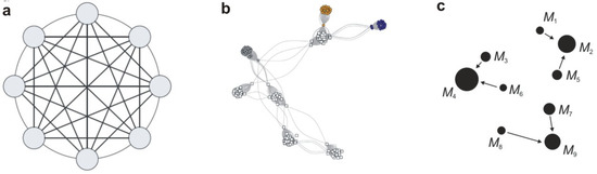
Figure 1.
Different nests used in specific methods or models (a) SOM-like [21] (b) Colobus network [60] (c) NOAH.
Hypothetically and in accordance with the heuristic methods described in Section 2, the behaviors presented above can be used in an algorithm (NOAH) that can describe not only groups of animals, but also technical systems containing parameters (factors) related to human behavior (like choice of transport means). Especially useful can be changeable leadership in the nest and the behaviors of followers. The parameters will be associated with “monkeys”—individuals in the nest that change their behavior (monkey position) according to specific procedures including leader creation, observations by followers, importance and hierarchy of individuals, dynamic changes in the nest, etc.
Changes to the nest will modify individuals (factors) before the algorithm stops. It will be possible to analyze and observe different sets of parameters (monkeys), their interactions, and their correlations. NOAH does not specify an optimal solution but shows possible datasets for comparison. It helps in choosing one or more. The operation of NOAH is very similar to the SOM (self-organized maps) concept, the stages of the blockchain, or the multiagent concept. A graphical representation of the exemplary methods is shown in Figure 1. Part (a) of this figure shows an SOM-like network, part (b) shows the colobus monkey nest described earlier, and part (c) shows the monkey nest and interactions between leaders (big black spots) and followers (little black spots) according to the NOAH concept.
Important for the application of NOAH in selected problems is the selection of parameters (factors) and their conversion into “monkeys”. Initially, the selection of parameters is made by an “expert” with the use of all of the available data. After the algorithm is stopped, the re-conversion procedure will follow. These elements will be described in Section 4 with a specific example. The basic and theoretical aspects of NOAH are presented here. Each monkey has a specific position in the nest that is variable. The monkey position values are limited to a range of 0 to 1 as defined by the procedures in NOAH.
A specific set of terms, parameters, and symbols used in NOAH is defined herein.
Nest (seat, habitat) is a set of individuals (representing factors in the model).
Position of the monkey in the nest, Mn, is a key variable in the algorithm. Each monkey changes its position in the nest, assuming the role of a leader or follower (representing variable values of factors and their importance in the model).
Steps (iterations) of changes in the nest, starting from zero, i = 0, are successive periods with a specific nest state (monkey position, i.e., factor values). The steps will continue until the socket is stable (will not change). See stopping criteria.
Importance of an individual, In, is a random variable indicating the subjective position of the monkey in the nest. The scope of this variable is determined by Formula (1).
Hierarchy of an individual, Hn: This is a variable indicating a more objective position of the individual in the nest, assuming an actual value of Mn, a random importance In, a moderated followers coefficient L, and a number of steps i. The hierarchy is calculated using Formula (2).
Followers coefficient (influence of leaders), L: This determines the time and efficiency of the algorithm (it should be precisely defined in accordance with the specification of the modeled problem). Its impact increases in subsequent iteration steps—see Formula (2). L values should oscillate around 1–3 (see example in Section 4).
Random hierarchy modifiers, Rn: These are used to modify the position of the monkey going to the next step of changes in the nest. The modifiers depend on the value of the hierarchy, taking into account the defined range of hierarchy modifiers according to Formula (3).
Range of hierarchy modifiers, Rmin and Rmax: This also determines the runtime and efficiency of the algorithm; the Rmin value should be negative and the Rmax value positive (see example in Section 4).
NOAH works according to the algorithm shown in Figure 2. The position of the monkey in the next step is calculated using Formula (4). The position is changed taking into account the values of random hierarchy modifiers with the restrictions determined by Formula (5).
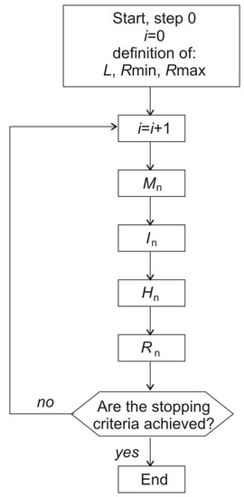
Figure 2.
NOAH algorithm.
The progressing steps create a changeable nest with individuals who change their positions. That means the changeable values of factors are considered in the model. The leaders (factors with higher importance) are identified, observed, and analyzed. The whole nest (set of all factors) can be analyzed too. The algorithm heads to the nest stability, which means reducing the changes in the monkey’s position during the steps. The tempo of such stabilization depends on the value of the followers coefficient and the range of hierarchy modifiers. However, specific stopping criteria are formulated. In each step the following “decisions measures” are calculated: M as the sum of all Mn, I as the sum of all In, H as the average from all Hn, and R as the average of all Rn. Consideration of these measures in the aspect of stopping criteria is shown in the example in Section 4.
The next steps of the algorithm create a changing nest with individuals of different positions. This refers to changes in the value of the factors included in the model. Leaders (factors of greater importance) are identified, monitored, and analyzed. The entire nest (set of all factors) can also be analyzed. The algorithm aims at nest stability, which means reducing the changes in the monkey’s position during steps. The pace of such stabilization depends on the value of the followers coefficient and the range of hierarchy modifiers. Specific stopping criteria have been formulated. At each step, the following “decision measures” are calculated: M as the sum of all Mn, I as the sum of all In, H as the average of all Hn, and R as the average of all Rn. The inclusion of these measures in terms of the stopping criteria is illustrated in the example in Section 4.
4. Application Example of NOAH
4.1. Case Study
The case study area is located near Wrocław, the fourth major city in Poland. Wrocław is the core of an agglomeration with approximately 1 million inhabitants. The Wrocław railway junction is large and forms the basis of the shape of the suburban railway system. This system is under construction, and several railway lines are being rebuilt or extended. In December 2021, the rebuilt line connecting Wrocław with Jelcz through the Czernica community was opened after 20 years without passenger transport. The occurrence of the reopening provides an opportunity for specific research, including testing of the NOAH algorithm. The use of NOAH allows for temporary changes to the rail network to be taken into account, e.g., the closure of a specific section of the line. The situation of the temporary closure of one railway connection makes it possible to observe all public transport connections between Wrocław and Jelcz using only one corridor.
Several factors and their collections are considered. Among them are new railroads, bus lines, and parking lots. These data were compared with the observed values of the number of passengers, etc. Figure 3 shows the map of the case study area, taking into account different types of railway lines (older ones in black, new ones in blue, and temporarily closed ones in red), two groups of bus lines (correlated with the railway line in green and competitive with red railways), target area in terms of the area of the Czernica commune, and car parks at railway stations in this area (park and ride, PR). Based on these conditions, 16 factors are formulated to be considered in the NOAH model.
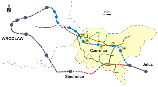
Figure 3.
The map of the case study area.
4.2. Factors and Their Conversion
A set of 16 factors was used in this case study (Table 2). Factors are divided into two groups: positive (nine factors) and negative (seven factors). Rising values of positive factors increase the total number of travelers (in all modes), and increasing values of negative factors reduce this number. This is a proposal used in this research considering specific assumptions (not defining the close set of factors and their role). For example, factors F2 and F3 are classified as “positive” according to an assumption of the offer presented by the rail operator having a higher number of places than the forecasted demand. In such an assumption, the trains will not become overcrowded. The higher number of passengers or people who get on the train will increase the use of suburban rail because of the creation of “good behavior” for new passengers. Conversion into monkeys and re-conversion differ depending on which group the factor belongs to. The set of factors adopted here is not complete in terms of all possible measures of the rail system, but it does contain exemplary, representative, and easy-to-collect data.
Table 2.
The factors considered in the case study.
Assuming (or identifying) a range of all factors is a necessary and important element of NOAH. The minimum and maximum values of the selected factors are necessary to calculate the monkey position value (Mn). Monkey positions correspond with the factors collected in Table 2. Two experiments are carried out in this case study. The first (Section 4.3) tests the volatility of the factor values. The second (Section 4.4) takes the actual factor values and compares them with the NOAH results. The conversion from F to M only occurs in the second experiment, but the re-conversion from M to F applies to both experiments. The following conversion formulas (6)–(7) and re-conversion formulas (8)–(9) are used depending on the specificity of the positive (FP) or negative (FN) factors. The mathematical conversion formulas are used impose monkey position values in the range of 0 to 1.
where:
FPmin to FPmax is the range of positive factors;
FNmax to FNmin is the range of negative factors.
Data for both experiments are summarized in Table 3. The “reference value” of a factor and the corresponding monkey position value show the actual (current) data. All factor values are commented on in Section 5.
Table 3.
The data for both experiments.
4.3. Experiment 1, Testing the Changeability of Factors’ Values
In this experiment, the initial values of all monkey positions are midway between the minimum and maximum, which is 0.500. The followers coefficient (L) is 1.5, and the range of hierarchy modifiers (Rmin, Rmax) are −0.3 and 0.3. These values were selected based on testing various algorithm stop criteria. This aspect is commented on in Section 5. The effect of the NOAH algorithm after 32 steps is shown in Figure 4.
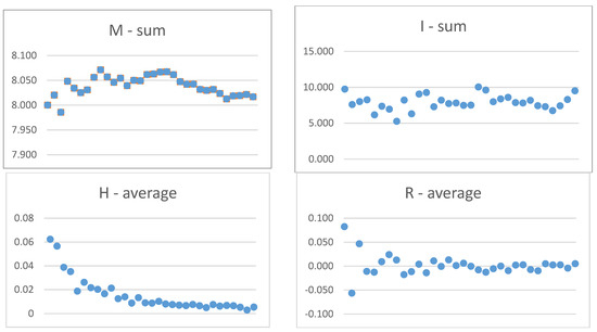
Figure 4.
Changes in decision measures during the steps in Experiment 1.
Because the initial monkey position value assumption is 0.5 and the number of monkeys considered is 16, the starting value of the first decision measure (M) is 8.0. The value of this measure is changed in the subsequent steps of the algorithm in accordance with the procedures described in Section 3. These changes should be observed in order to formulate the algorithm stopping criteria. One such criterion could be the difference between the M values in the following steps. When this difference reaches a predetermined minimum, the algorithm stops. We observe “stabilization in the nest”.
The second decision measure is the sum of importance values (I). Because each individual’s value for importance is random, the measure I varies from step to step but fluctuates around an average of 8.0. Observing the changes in the value of I makes sense in order to formulate the second algorithm stopping criterion. If you change this value significantly, you can stop the algorithm or ignore this particular step. Here we see “a remarkable change of subjective meaning in the nest”.
The average value of the hierarchy (H) is the third decision measure. This value drops to zero. Achieving the assumed minimum value may terminate the algorithm’s work. A similar situation takes place in the next decision measure—the average value of the random hierarchy modifier (R). It is possible to use only one decision measure and only one stop criterion, but the observation of all of them increases the set of analyzed solutions. In this experiment, stabilization in the socket was achieved after 32 steps, and the algorithm was completed. The values of all NOAH parameters for all monkeys and the decision measures in the final step are presented in Table 4. This table also shows the recalculated values of the analyzed factors as a set characterizing the final step of the algorithm. The interpretation of the coefficient values is presented in Section 5
Table 4.
The results of the first experiment.
4.4. Experiment 2, Considering the Real Data
In this experiment, the initial values of the monkeys are calculated according to actual (reference) factor values (see Table 3). The values of the followers coefficient and hierarchy modifier ranges are the same as in Experiment 1. The effect of the NOAH algorithm after 32 steps is shown in Figure 5. The same four decision measures and stopping criteria were also used as in Experiment 1. The values of all NOAH parameters for all monkeys and decision measures in the final step are presented in Table 5. This table also shows the re-converted values of the analyzed factors as a set characterizing the final step of the algorithm. The interpretation of the factor values is presented in Section 5.
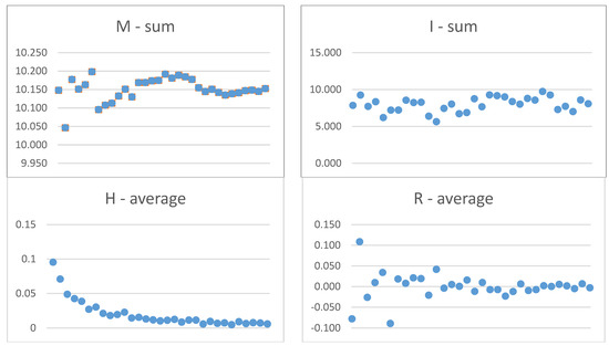
Figure 5.
Changes in decision measures during the steps in Experiment 2.
Table 5.
The results of the second experiment.
5. Discussion
Table 6 summarizes the important data for all factors. The minimum, maximum, reference (actual), and final values from both experiments are shown. The reference values correspond to the observed (measured) situations. Measurements and data collection were performed in the spring of 2022. The minimum and maximum values are calculated or assumed according to physical conditions or other possibilities. For example, “percentage of spaces occupied” (F4) can of course vary between 0 and 100%, and “parking volume on PR” (F7) can vary between 0 and 100, the upper limit being the actual number of parking spaces in all of the considered locations. The “cost” (F10) could vary from PLN 4.6 to 12.0, which results from the comparison of various fees in the considered journeys between the origin and the destination; “travel times” (F12–F14) oscillate between values obtained from measurements or calculated taking into account the possible speeds.
Table 6.
Set of values for all factors.
The values obtained in the experiments depend on the values of the parameters adopted in the algorithm: the followers coefficient (L) and the range of hierarchy modifiers (Rmin, Rmax). These values may vary depending on the specifics of the problem under consideration (e.g., depending on a number of factors) and should be tested in the experimental phase of the research. Finally, the values were selected—L = 1.5, Rmin = −0.3 and Rmax = 0.3—as the best according to the decision measure change process. The impact of the abovementioned parameters on the results of NOAH requires further research and will be explored in the future.
The factors values obtained from the experiments should be analyzed as a complex set of parameters. In both experiments, sufficient numbers of trips (F1) and stops (F5) were identified in relation to the values of the other factors. These values led to an intuitive decrease in the number of passengers during the day (F2). Comparing these values with the stable number of residents (F6), there is a need to increase the role of the delivery system. The delivery system is represented here by factors including cars in PR (F7) and passengers arriving from correlated forms of public transport (F8). The travel cost (F10) should be lower. The conditions tested above also show a lower number of journeys by means that compete with rail, both with private cars (F16) and buses (F15).
Some results differ in both experiments. Because the first experiment starts with the “average” values of the factors, the results are close to the middle between the minimum and the maximum. This shows the potential NOAH effect but is not of practical use. The results of the second experiment are more realistic and allow you to judge the real conditions. The maintenance of a clear difference between the travel time of rail travel and those of competitive forms is particularly visible. The results show the possibilities of further use of the constructed methodology and algorithm. For example, it is possible to test other numbers of residents (F6) or numbers of departures (F1). It is also possible to test different values of the minimum and maximum factors. They should allow the modeling of various conditions in the suburban rail system and the observation of correlations between all factors. Initial values of the abovementioned parameters should be carefully collected. This limitation requires further work to be overcome.
The obtained results correspond with actual topics involved in the interdisciplinary field of sustainable urban planning and transport development. Significantly, connection with heuristics used in analyses of transportation and railway systems [64,65] occurred. This aspect shows the potential of the proposed algorithm and methodology to be developed in other studies not only connected with railway systems and not only in transportation engineering.
6. Conclusions
The parameters describing a suburban rail system have different characteristics. The set of possible factors is not precisely defined, and the data collection process has specific problems. Some data are incomplete, while others contain errors. The influence of each selected factor and its importance are not fully understood. Therefore, modeling and analysis of suburban rail systems requires specific methods that also take into account human behavior. Here, heuristics as a holistic tool can help in the analysis of possible correlations between factors, as well as be helpful in the decision-making process. The novel method presented here allows using an open set of data. The factors could be different and somewhat “chaotic” at first sight (as in the presented experiments). This is the key innovation in analyses of “technical systems” like the suburban railways considered here.
The main advantage of the proposed method is the creation of the possibility to observe various sets of data and their interactions without precise knowledge about the influence of a specific factor on the result. The data (describing the transportation systems) depend partially on human decisions. For example, the choice of the mode of transport could be a reaction to the behaviors of other people (neighbors, social media groups). So, an individual can observe and copy leaders as a follower. The use of the specific transport means influencing the number of passengers or parking volume in PR has some uncertainties and could be modeled using heuristics.
NOAH, which is inspired by the behavior of groups of monkeys, especially taking into account dynamic changes in leadership, is likely to be useful in specific technical problems where physical parameters (such as the number of departures or stops) are compared with human decisions moderated by travel time, prices, etc. The basic definitions, the procedures, the algorithm, and the potential application of NOAH are illustrated in simple examples with a relatively small set of factors. The NOAH algorithm modifies the values of factors in a heuristic way and shows possible solutions that could be introduced in reality. This method created originally by the author is quite similar to swarm intelligence algorithms (like PSO and ACO) but contains new elements based on specific behaviors of monkeys which were described in Section 3.
Strict comparison of this new method with others is not possible because of the other goals of those methods. The heuristics search mainly for optimal solutions. NOAH can compare factors, not showing the best result. This is an intentional assumption representing the difficulty of evaluation of data by an individual person. Thus, the evaluation of the effectiveness of the proposed method is difficult, especially in the present stage of research. The study introduced in one of the Polish agglomerations will be continued and should formulate remarks to modify selected elements of the transport system (e.g., number of departures or cost) with the observation of changes in other factors. When the obtained results are similar to the model, NOAH will be effective.
The presented material introduces the new algorithm by showing its procedures that can allow for its use in similar problems. This could test obtained assumptions and improve procedures in the future. Future works should contain influence analyses of the parameters adopted in the algorithm (the followers coefficient and the range of hierarchy modifiers), other (broader) sets of factors, and comprised studies in other areas. The NOAH method could be also used for other problems where incomplete and different data make observations of technical systems difficult.
Funding
This research received no external funding.
Institutional Review Board Statement
Not applicable.
Informed Consent Statement
Not applicable.
Data Availability Statement
Not applicable.
Conflicts of Interest
The author declares no conflict of interest.
References
- Canca, D.; De-Los-Santos, A.; Laporte, G.; Mesa, J.A. An adaptive neighborhood search metaheuristic for the integrated railway rapid transit network design and line planning problem. Comput. Oper. Res. 2017, 78, 1–14. [Google Scholar] [CrossRef]
- Yan, F.; Goverde, R.M.P. Combined line planning and train timetabling for strongly heterogeneous railway lines with direct connections. Transp. Res. Part B Methodol. 2019, 127, 20–46. [Google Scholar] [CrossRef]
- Hickish, B.; Fletcher, D.I.; Harrison, R.F. Investigating Bayesian Optimization for rail network optimization. Int. J. Rail Transp. 2020, 8, 307–323. [Google Scholar] [CrossRef]
- Schlechte, T.; Borndörfer, R.; Erol, B.; Graffagnino, T.; Swarat, E. Micro–macro transformation of railway networks. J. Rail Transp. Plan. Manag. 2011, 1, 38–48. [Google Scholar] [CrossRef]
- Weik, N.; Warg, J.; Johansson, I.; Bohlin, M.; Nießen, N. Extending UIC 406-based capacity analysis—New approaches for railway nodes and network effects. J. Rail Transp. Plan. Manag. 2020, 15, 100199. [Google Scholar] [CrossRef]
- Ahmed, C.; Nur, K.; Ochieng, W. GIS and genetic algorithm based integrated optimization for rail transit system planning. J. Rail Transp. Plan. Manag. 2020, 16, 100222. [Google Scholar] [CrossRef]
- Dong, X.; Li, D.; Yin, Y.; Ding, S.; Cao, Z. Integrated optimization of train stop planning and timetabling for commuter railways with an extended adaptive large neighborhood search metaheuristic approach. Transport. Res. C Emerg. Technol. 2020, 117, 102681. [Google Scholar] [CrossRef]
- Qiannan, W.; Yang, L.; Pengrui, D. Optimization of urban rail transit station spacing for minimizing passenger travel time. J. Rail Transp. Plan. Manag. 2022, 22, 100317. [Google Scholar] [CrossRef]
- Binder, S.; Maknoon, M.Y.; Sharif Azadeh, S.; Bierlaire, M. Passenger-centric timetable rescheduling: A user equilibrium approach. Transport. Res. Part C Emerg. Technol. 2021, 132, 103368. [Google Scholar] [CrossRef]
- Jamili, A.; Pourseyed Aghaee, M. Robust stop-skipping patterns in urban railway operations under traffic alteration situation. Transport. Res. Part C Emerg. Technol. 2015, 61, 63–74. [Google Scholar] [CrossRef]
- Shang, P.; Li, R.; Liu, Z.; Yang, L.; Wang, Y. Equity-oriented skip-stopping schedule optimization in an oversaturated urban rail transit network. Transport. Res. Part C Emerg. Technol. 2018, 89, 321–343. [Google Scholar] [CrossRef]
- Wang, Y.; D’Ariano, A.; Yin, J.; Meng, L.; Tao, T.; Ning, B. Passenger demand oriented train scheduling and rolling stock circulation planning for an urban rail transit line. Transp. Res. Part B Methodol. 2018, 118, 193–227. [Google Scholar] [CrossRef]
- Jensen, L.W.; Landex, A.; Nielsen, O.A.; Kroon, L.G.; Schmidt, M. Strategic assessment of capacity consumption in railway networks: Framework and model. Transp. Res. Part C Emerg. Technol. 2017, 74, 126–149. [Google Scholar] [CrossRef]
- Yin, J.; D’Ariano, A.; Wang, Y.; Yang, L.; Tang, T. Timetable coordination in a rail transit network with time-dependent passenger demand. Eur. J. Oper. Res. 2021, 295, 183–202. [Google Scholar] [CrossRef]
- Zhang, T.; Li, D.; Qiao, Y. Comprehensive optimization of urban rail transit timetable by minimizing total travel times under time-dependent passenger demand and congested conditions. Appl. Math. Model. 2018, 58, 421–446. [Google Scholar] [CrossRef]
- Zhang, Y.; D’Ariano, A.; He, B.; Peng, Q. Microscopic optimization model and algorithm for integrating train timetabling and track maintenance task scheduling. Transp. Res. Part B Methodol. 2019, 127, 237–278. [Google Scholar] [CrossRef]
- Zhang, Y.; Peng, Q.; Yao, Y.; Zhang, X.; Zhou, X. Solving cyclic train timetabling problem through model reformulation: Extended time-space network construct and Alternating Direction Method of Multipliers methods. Transp. Res. Part B Methodol. 2019, 128, 344–379. [Google Scholar] [CrossRef]
- Zhang, Q.; Lusby, R.M.; Shang, P.; Zhu, X. A heuristic approach to integrate train timetabling, platforming, and railway network maintenance scheduling decisions. Transp. Res. Part B Methodol. 2022, 158, 210–238. [Google Scholar] [CrossRef]
- Zhao, S.; Yang, H.; Wu, Y. An integrated approach of train scheduling and rolling stock circulation with skip-stopping pattern for urban rail transit lines. Transp. Res. Part C Emerg. Technol. 2021, 128, 103170. [Google Scholar] [CrossRef]
- Whitbrook, A.; Meng, Q.; Chung, P.W.H. Reliable, Distributed Scheduling and Rescheduling for Time-Critical, Multiagent Systems. IEEE Trans. Autom. Sci. Eng. 2018, 15, 732–747. [Google Scholar] [CrossRef]
- Zheng, Y.-J.; Ling, H.-F.; Shi, H.-H.; Chen, H.-S.; Chen, S.-Y. Emergency railway wagon scheduling by hybrid biogeography-based optimization. Comput. Oper. Research 2014, 43, 1–8. [Google Scholar] [CrossRef]
- Satoshi, K.; Koichi, S.; Shingo, H.; Norio, T. An optimal delay management algorithm from passengers’ viewpoints considering the whole railway network. J. Rail Transp. Plan. Manag. 2011, 1, 25–37. [Google Scholar] [CrossRef]
- Samà, M.; Pellegrini, P.; D’Ariano, A.; Rodriguez, J.; Pacciarelli, D. On the tactical and operational train routing selection problem. Transp. Res. Part C Emerg. Technol. 2017, 76, 1–15. [Google Scholar] [CrossRef]
- Oneto, L.; Fumeo, E.; Clerico, G.; Canepa, R.; Papa, F.; Dambra, C.; Mazzino, N.; Anguita, D. Dynamic Delay Predictions for Large-Scale Railway Networks: Deep and Shallow Extreme Learning Machines Tuned via Thresholdout. IEEE Trans. Syst. Man Cybern. Systems 2017, 47, 2754–2767. [Google Scholar] [CrossRef]
- Xiao, X.; Jia, L.; Wang, Y. Correlation between heterogeneity and vulnerability of subway networks based on passenger flow. J. Rail Transp. Plan. Manag. 2018, 8, 145–157. [Google Scholar] [CrossRef]
- Shen, W.; Xiao, W.; Wang, X. Passenger satisfaction evaluation model for Urban rail transit: A structural equation modeling based on partial least squares. Transp. Policy 2016, 46, 20–31. [Google Scholar] [CrossRef]
- Wu, J.; Sun, H.; Wang, D.Z.W.; Zhong, M.; Han, L.; Gao, Z. Bounded-rationality based day-to-day evolution model for travel behavior analysis of urban railway network. Transp. Res. Part C Emerg. Technol. 2013, 31, 73–82. [Google Scholar] [CrossRef]
- Liu, Y.; Liu, Z.; Jia, R. DeepPF: A deep learning based architecture for metro passenger flow prediction. Transp. Res. Part C Emerg. Technol. 2019, 101, 18–34. [Google Scholar] [CrossRef]
- Liu, T.; Cats, O.; Gkiotsalitis, K. A review of public transport transfer coordination at the tactical planning phase. Transp. Res. Part C Emerg. Technol. 2021, 133, 103450. [Google Scholar] [CrossRef]
- Hansson, J.; Pettersson-Löfstedt, F.; Svensson, H.; Wretstrand, A. Replacing regional bus services with rail: Changes in rural public transport patronage in and around villages. Transp. Policy 2021, 101, 89–99. [Google Scholar] [CrossRef]
- Wei, S.; Zheng, W.; Wang, L. Understanding the configuration of bus networks in urban China from the perspective of network types and administrative division effect. Transp. Policy 2021, 104, 1–17. [Google Scholar] [CrossRef]
- Ngo, N.S.; Götschi, T.; Clark, B.Y. The effects of ride-hailing services on bus ridership in a medium-sized urban area using micro-level data: Evidence from the Lane Transit District. Transp. Policy 2021, 105, 44–53. [Google Scholar] [CrossRef]
- Behrends, S. Burden or opportunity for modal shift?—Embracing the urban dimension of intermodal road-rail transport. Transp. Policy 2017, 59, 10–16. [Google Scholar] [CrossRef]
- Stead, A.D.; Wheat, P.; Smith, A.S.J.; Ojeda-Cabral, M. Competition for and in the passenger rail market: Comparing open access versus franchised train operators’ costs and reliability in Britain. J. Rail Transp. Plan. Manag. 2019, 12, 100142. [Google Scholar] [CrossRef]
- Yang, A.; Wang, B.; Huang, J.; Li, C. Service replanning in urban rail transit networks: Cross-line express trains for reducing the number of passenger transfers and travel time. Transport. Res. Part C 2020, 115, 102629. [Google Scholar] [CrossRef]
- Lianhua, T.; Xingfang, X. Optimization for operation scheme of express and local trains in suburban rail transit lines based on station classification and bi-level programming. J. Rail Transp. Plan. Manag. 2022, 21, 100283. [Google Scholar] [CrossRef]
- Chen, X.; Lin, X.; He, F.; Li, M. Modeling and control of automated vehicle access on dedicated bus rapid transit lanes. Transp. Res. Part C Emerg. Technol. 2020, 120, 102795. [Google Scholar] [CrossRef]
- Tang, R.; De Donato, L.; Bešinović, N.; Flammini, F.; Goverde, R.M.P.; Lin, Z.; Liu, R.; Tang, T.; Vittorini, V.; Wang, Z. A literature review of Artificial Intelligence applications in railway systems. Transp. Res. Part C Emerg. Technol. 2022, 140, 103679. [Google Scholar] [CrossRef]
- López, D.; Farooq, B. A multi-layered blockchain framework for smart mobility data-markets. Transp. Res. Part C Emerg. Technol. 2020, 111, 588–615. [Google Scholar] [CrossRef]
- Khisty, C.J.; Arslan, T. Possibilities of steering the transportation planning process in the face of bounded rationality and unbounded uncertainty. Transp. Res. Part C Emerg. Technol. 2005, 13, 77–92. [Google Scholar] [CrossRef]
- Li, H.; He, F.; Lin, X.; Wang, Y.; Li, M. Travel time reliability measure based on predictability using the Lempel–Ziv algorithm. Transp. Res. Part C Emerg. Technol. 2019, 101, 161–180. [Google Scholar] [CrossRef]
- Kahneman, D. Thinking Fast and Slow; Farrar, Straus and Giroux: New York, NY, USA, 2013; ISBN -100374533555. [Google Scholar]
- Lau, H.C.; Raidl, G.R.; Van Hentenryck, P. New developments in metaheuristics and their applications. J. Heuristics 2016, 22, 359–363. [Google Scholar] [CrossRef][Green Version]
- Xavier, E.A.; Xavier, V.L. Flying elephants: A general method for solving non-differentiable problems. J. Heuristics 2016, 22, 649–664. [Google Scholar] [CrossRef]
- Martinelli, D.R.; Teng, H. Optimization of railway operations using neural networks. Transp. Res. Part C Emerg. Technol. 1996, 4, 33–49. [Google Scholar] [CrossRef]
- Fischetti, M.; Monaci, M. Proximity search heuristics for wind farm optimal layout. J. Heuristics. 2016, 22, 459–474. [Google Scholar] [CrossRef]
- Teodorović, D. Swarm intelligence systems for transportation engineering: Principles and applications. Transp. Res. Part C Emerg. Technol. 2008, 16, 651–667. [Google Scholar] [CrossRef]
- Venter, G.; Sobieszczanski-Sobieski, J. Multidisciplinary optimization of a transport aircraft wing using particle swarm optimization. Struct. Multidisc. Optim. 2004, 26, 121–131. [Google Scholar] [CrossRef]
- Steiger, E.; Resch, B.; de Albuquerque, J.P.; Zipf, A. Mining and correlating traffic events from human sensor observations with official transport data using self-organizing-maps. Transp. Res. Part C Emerg. Technol. 2016, 73, 91–104. [Google Scholar] [CrossRef]
- Cesme, B.; Furth, P.G. Self-organizing traffic signals using secondary extension and dynamic coordination. Transp. Res. Part C Emerg. Technol. 2014, 48, 1–15. [Google Scholar] [CrossRef]
- Hua, G.; Zhu, L.; Wu, J.; Shen, C.; Zhou, L.; Lin, Q. Blockchain-Based federated learning for intelligent control in heavy haul railway. IEEE Access 2020, 8, 176830–176839. [Google Scholar] [CrossRef]
- Kawaji, H.; Takenaka, Y.; Matsuda, H. Graph-based clustering for finding distant relationships in a large set of protein sequences. Bioinformatics 2004, 20, 243–252. [Google Scholar] [CrossRef]
- Paradis, E.; Claude, J.; Strimmer, K. APE: Analyses of phylogenetics and evolution in R language. Bioinformatics 2004, 20, 289–290. [Google Scholar] [CrossRef]
- Simon, D. Biogeography-Based optimization. IEEE Trans. Evol. Computation 2008, 12, 702–713. [Google Scholar] [CrossRef]
- Nakamoto, S. Bitcoin: A Peer-to-Peer Electronic Cash System; Technical Report; Bitcoin.org: 2008. Available online: https://bitcoin.org/bitcoin.pdf (accessed on 22 October 2022).
- Decellieres, M.; Zuberbühler, K.; León, J. Habitat-dependent intergroup hostility in Diana monkeys, Cercopithecus diana. Anim. Behav. 2021, 178, 95–104. [Google Scholar] [CrossRef]
- Gareta García, M.; Farine, D.R.; Brachotte, C.; Borgeaud, C.; Bshary, R. Wild female vervet monkeys change grooming patterns and partners when freed from feeding constraints. Anim. Behav. 2021, 181, 117–136. [Google Scholar] [CrossRef]
- Leca, J.-B.; Gunst, N.; Thierry, B.; Petit, O. Distributed leadership in semifree-ranging white-faced capuchin Monkeys. Anim. Behav. 2003, 66, 1045–1052. [Google Scholar] [CrossRef]
- Miller, C.M.; Snyder-Mackler, N.; Nguyen, N.; Fashing, P.J.; Tung, J.; Wroblewski, E.E.; Gustison, M.L.; Wilson, M.L. Extragroup paternity in gelada monkeys, Theropithecus gelada, at Guassa, Ethiopia and a comparison with other primates. Anim. Behav. 2021, 177, 277–301. [Google Scholar] [CrossRef]
- Wikberg, E.C.; Christie, D.; Sicotte, P.; Ting, N. Interactions between social groups of colobus monkeys (Colobus vellerosus) explain similarities in their gut microbiomes. Anim. Behav. 2020, 163, 17–31. [Google Scholar] [CrossRef]
- Scelza, B.A.; Prall, S.P.; Blumenfield, T.; Crittenden, A.N.; Gurven, M.; Kline, M.; Koster, J.; Kushnick, G.; Mattison, S.M.; Pillsworth, E.; et al. Patterns of paternal investment predict cross-cultural variation in jealous response. Nat. Hum. Behav. 2019, 4, 20–26. [Google Scholar] [CrossRef]
- Scelza, B.A.; Prall, S.P.; Swinford, N.; Gopalan, S.; Atkinson, E.G.; Mcelreath, R. High rate of extrapair paternity in a human population demonstrates diversity in human reproductive strategies. Sci. Adv. 2020, 6, 1–7. [Google Scholar] [CrossRef]
- Henrich, J.; Heine, S.J.; Norenzayan, A. The weirdest people in the world? Behav. Brain Sci. 2010, 33, 61–83. [Google Scholar] [CrossRef] [PubMed]
- Li, G.; Zhang, R.; Guo, S.; Zhang, J. Analysis of ride-hailing passenger satisfaction and life satisfaction based on a MIMIC model. Sustainability 2022, 14, 10954. [Google Scholar] [CrossRef]
- Gong, W.; Li, J.; Ng, M.K. Deciphering property development around high-speed railway stations through land value capture: Case studies in Shenzhen and Hong Kong. Sustainability 2021, 13, 12605. [Google Scholar] [CrossRef]
Disclaimer/Publisher’s Note: The statements, opinions and data contained in all publications are solely those of the individual author(s) and contributor(s) and not of MDPI and/or the editor(s). MDPI and/or the editor(s) disclaim responsibility for any injury to people or property resulting from any ideas, methods, instructions or products referred to in the content. |
© 2022 by the author. Licensee MDPI, Basel, Switzerland. This article is an open access article distributed under the terms and conditions of the Creative Commons Attribution (CC BY) license (https://creativecommons.org/licenses/by/4.0/).