The Spatiotemporal Characteristics of Water Quality and Main Controlling Factors of Algal Blooms in Tai Lake, China

Abstract

Taking Tai Lake in China as the research area, a 3D water environment mathematical model was built. Combined with the LHS and Morris uncertainty and sensitivity analysis methods, the uncertainty and sensitivity analysis of total phosphorus (TP), total nitrogen (TN), dissolved oxygen (DO), and chlorophyll a (Chl-a) were carried out. The main conclusions are: (1) The performance assessment of the 3D water environment mathematical model is good (R² and NSE > 0.8) and is suitable for water quality research in large shallow lakes. (2) The time uncertainty study proves that the variation range of Chl-a is much larger than that of the other three water quality parameters and is more severe in summer and autumn. (3) The spatial uncertainty study proves that Chl-a is mainly present in the northwest lake area (heavily polluted area) and the other three water quality indicators are mainly present in the center. (4) The sensitivity results show that the main controlling factors of DO are ters (0.15) and kmsc (0.12); those of TN and TP are tetn (0.58) and tetp (0.24); and those of Chl-a are its own growth rate (0.14), optimal growth temperature (0.12), death rate (0.12), optimal growth light (0.11), and TP uptake rate (0.11). Thus, TP control is still the key treatment method for algal blooms that can be implemented by the Chinese government.

1. Introduction

Tai Lake is a typical large shallow lake; it is the third largest freshwater lake in China and is of important social value [1]. A water crisis due to an algae outbreak in 2007 alarmed the Chinese government. It has been more than 10 years since the cyanobacteria outbreak in Tai Lake, and algal blooms have appeared less often after the Chinese government’s treatment of the lake in the years following the crisis [2]. However, ten years later, in 2017, another outbrak of algae and a rebound of the total phosphorus concentration meant that the Chinese government and scientists lost control of the situation. It is well known that the presence of nutrients such as nitrogen (N) and phosphorus (P) lead to algal blooms [3]; therefore, it is very important to determine the spatiotemporal characteristics of the main general water quality indicators (TN, TP, and DO) in Tai Lake and the key control factors of algal blooms (Chl-a) through scientific methods so that we can explain the phenomenon better and provide more scientific support for the management of other large shallow lakes in the world.

Mathematical models are used by many researchers as an important analysis method [4,5]. The integrity and accuracy of these models have also improved rapidly with the development of other disciplines. In the field of water quality models, the main models include the Environmental Fluid Dynamics Code (EFDC), MIKE, the Water Ecosystems Tool (WET), Delft3D, and CE-QUAL-W2. The EFDC is funded by the U.S. Environmental Protection Agency (EPA). Its code is open source, but a fee must be paid to access the complete operating system. Successful case studies have been conducted in many lakes such as Tai Lake and Dianchi Lake in China [6]. MIKE was developed by the Danish company DHI. It is currently used in many lakes and rivers around the world, and is also listed as an official environmental assessment model in China. The technology is very mature and the interface is very smart, but the disadvantage is that the code is not open source and the usage fee is very high [7,8]. WET was developed by Aarhus University in Denmark based on the original FABM model. Its code and use are free, but, currently, it lacks two-dimensional and three-dimensional modules, and there are certain application defects [9,10]. Delft3D was developed by Delft University in the Netherlands. The code and its use are free. Its main advantage lies in its hydrodynamics, but it has lagged behind other models in terms of the simulation of water quality and algae in recent years [11]. CE-QUAL-W2 is a two-dimensional water environment mathematical model funded by the American Society of Military Engineers, but due to maintenance problems it has been used less and less in recent years [12]. In this study, we chose to use MIKE3 (one style based on MIKE) so that we could have a strong foundation for the uncertainty and sensitivity analyses we aimed to conduct in the next step.

In order to study the spatiotemporal characteristics and main controlling factors of water quality in Tai Lake, we used uncertainty and sensitivity analysis methods. Currently, the most common methods used in uncertainty and sensitivity analyses include the Monte Carlo method [13], Latin hypercube sampling (LHS) [14], the Morris method [15], the standardized rank regression coefficient (SRRC) method [16], the Sobol method [17], the generalized likelihood uncertainty estimation (GLUE) method [18], the shuffled complex evolution algorithm (SCE-UA) method [19], and the extended Fourier amplitude sensitivity test (EFAST) [20]. When there are too many parameters, the results of GLUE and SRRC analyses will contain large errors; nevertheless, the Morris method can make a good distinction between multiple parameters, but the original Morris method has certain deficiencies in terms of specific quantification [21]. Meanwhile, EFAST and Sobol require a large number of repeated model calculations, which seriously limit the effectiveness of the research [22,23]. In order to solve these problems, many scholars [24,25], in recent years, have conducted comparative research on related methods (

Table 1. Introduction to the uncertainty and sensitivity analysis methods.

Method	Name	Advantages	Limitations
Uncertainty analysis methods	Monte Carlo	Overcomes the shortcomings of the first-order error analysis	Low sampling and calculation efficiency Local aggregation errors may occur Not suitable for highly nonlinear and variable skewing distribution models
	LHS	Sampling speed and quality can be guaranteed Saving uncertainty analysis time	Still sorted by credibility, which is slightly inaccurate with insufficient reliability
	GLUE	Improves accuracy and reliability judgment due to likelihood value	Requires an excessive number of calculations Results affected by subjectivity
Sensitivity analysis methods	Morris	Requires few calculations The interactions between the parameters can be analyzed after improvement	Quantitative research is insufficient
	SRRC	Suitable for linear parameter group studies	Not suitable for the study of highly nonlinear parameters
	Sobol	Research on precise simulation of multidimensional nonlinear parameters	Requires an excessive number of calculations
	EFAST	The number of calculations is reduced as compared with the Sobol method	Requires an excessive number of calculations
	RSA	Fewer requirements and intuitive results	Cannot evaluate interactions between parameters

). Among them, Li et al. (2015) [26] used LHS to carry out sampling and uncertainty analyses of the hydrodynamic parameters of Tai Lake and combined LHS with SRRC to perform a parameter sensitivity analysis; it was found that this method was well suited to scenarios with few parameters and without a nonlinear relationship, but there was still no definite proof that it could be applied to a nonlinear situation with multiple parameters. Jiang et al. (2018) [18] used the GLUE uncertainty analysis and the regionalized sensitivity analysis (RSA) method to simulate the ecological parameters of Tai Lake and found that algae growth was mainly related to the parameters related to hydrodynamics, light, and temperature. They suggested the addition of zooplankton research modules in future studies. Yi et al. (2016) [27] simulated the ecological parameters of Dianchi Lake through the LHS, SRRC, and Morris methods, and found that the parameters had a significant effect on algae, spatially and at different times. They also showed that the research in this area was very important for the further development of the model.

The LHS used in this study was first optimized according to the Monte Carlo method by McKay [28]. This method solves the problem of uneven sampling, speeds up the sampling rate, and guarantees the samples are of high quality. This method has also been widely used in uncertainty analysis problems [29,30]. The improved Morris method [31] can qualitatively describe the sensitivity of each parameter to different indicators but can also analyze the degree of nonlinear correlation among different parameters, providing a new research foundation for the study of multidimensional, non-correlated parameter sensitivity. According to the literature, the Morris method requires a small sample size, which can minimize the workload for a computer. It has also been shown, through a comparison of global sensitivity analysis methods, that the Morris method is superior to the EFAST and SRRC methods for fitting multiple nonlinear parameters [32]. For a hydrodynamic ecological model, due to the high parameter dimension and the complicated correlations between each parameter [33], as well as the problem of calculating the load in temporal and spatial law research, we used the LHS and Morris methods to study and analyze the uncertainty and sensitivity of the parameters.

In order to calculate the precise spatiotemporal characteristics of the four water quality indicators in Tai Lake (2017) and to give a scientific explanation of the algal bloom in 2017, we combined the 3D environment mathematical model with the LHS and Morris methods in this research. We hope that the results not only explain the phenomenon well but also provide methodological ideas for research on the water environments in other large shallow lakes.

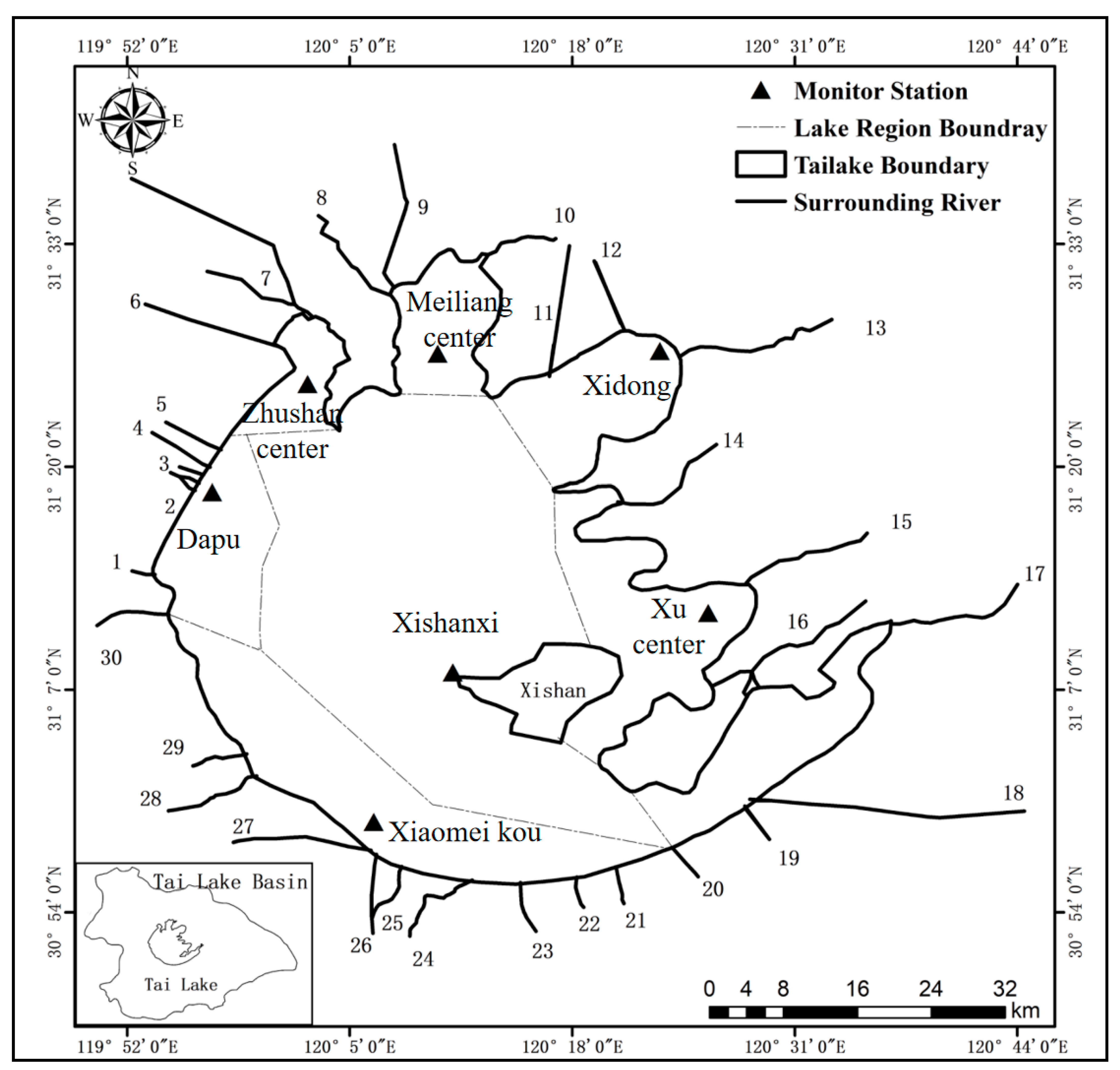
2. Study Area

Tai Lake, the third largest lake in China, is located between Jiangsu Province, Zhejiang Province, and Shanghai. The water surface area and basin area are 2338 km² and 36,900 km², respectively [34]. Thirty main rivers flow into the lake, which has an average depth of 1.9 m. Southeast and northwest winds usually prevail in summer and winter, respectively. The mean annual precipitation was 1245 mm from 2007 to 2017, and the mean annual air temperature was 16 °C from 2007 to 2017 [35,36,37]. This study established seven monitoring stations, each representing one of the seven main regions in the lake, for simulation research (Figure 1) to complete an analysis of the entire lake.

3. Methodology

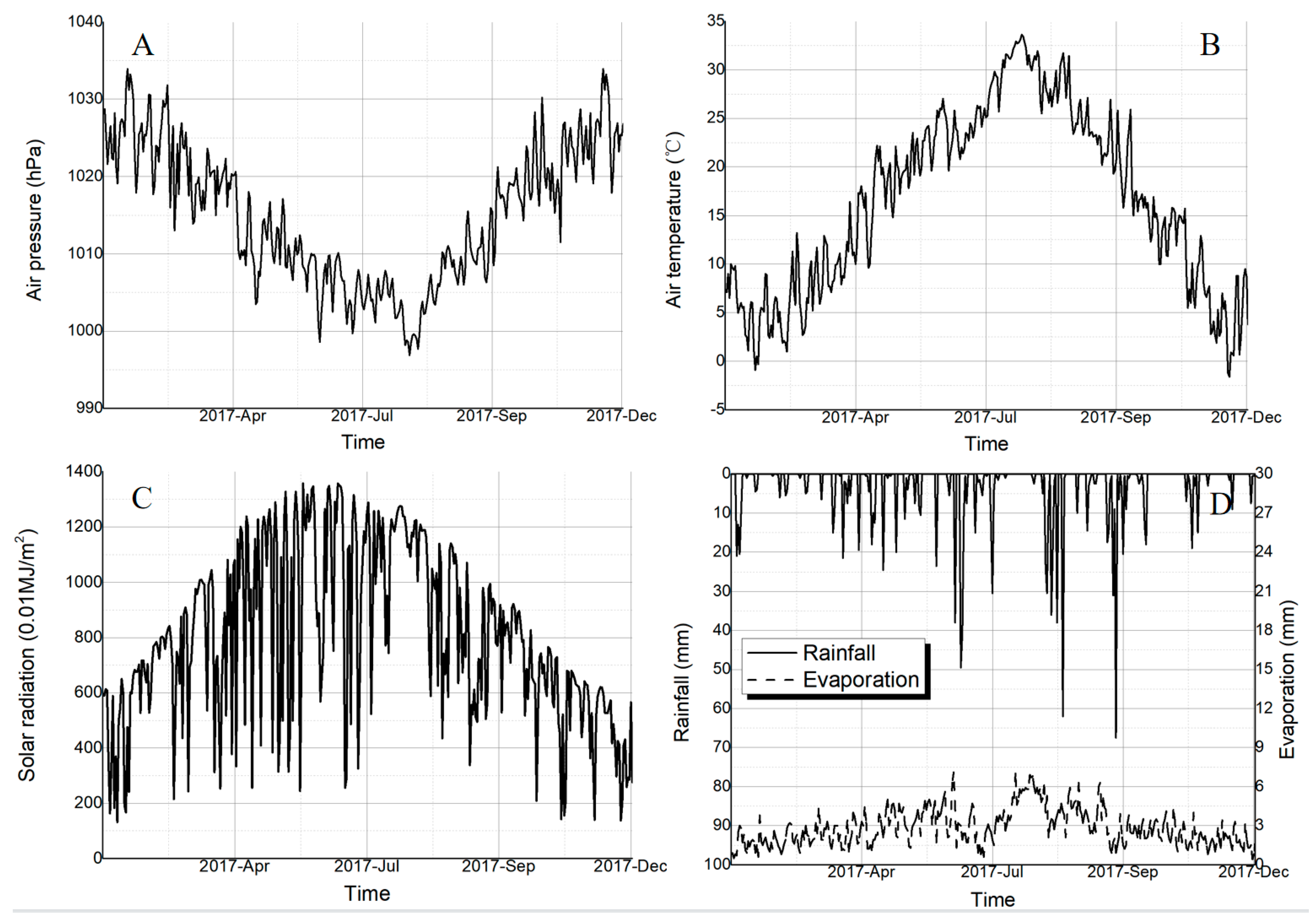
3.1. Data Collection

The discharge and wind field information of the rivers’ input and output during the simulation period were obtained from the online data (http://www.tba.gov.cn/, accessed on 26 April 2022) published monthly by the Tai lake Basin Administration of the Ministry of Water Resources of China. The input and the output water amounts in 2017 were around 11.11 billion m³ and 10.27 billion m³, respectively. The water quality data were obtained from the monthly monitoring data collected by local governments and the supplementary data from the Tai Lake Basin Administration of the Ministry of Water Resources of China. They are shown in the Calibration and Validation section. Meteorological data (Figure 2), including air pressure, temperature, solar radiation, and rainfall–evaporation, are published daily on the China Meteorological website (http://www.weather.com.cn/, accessed on 26 April 2022).

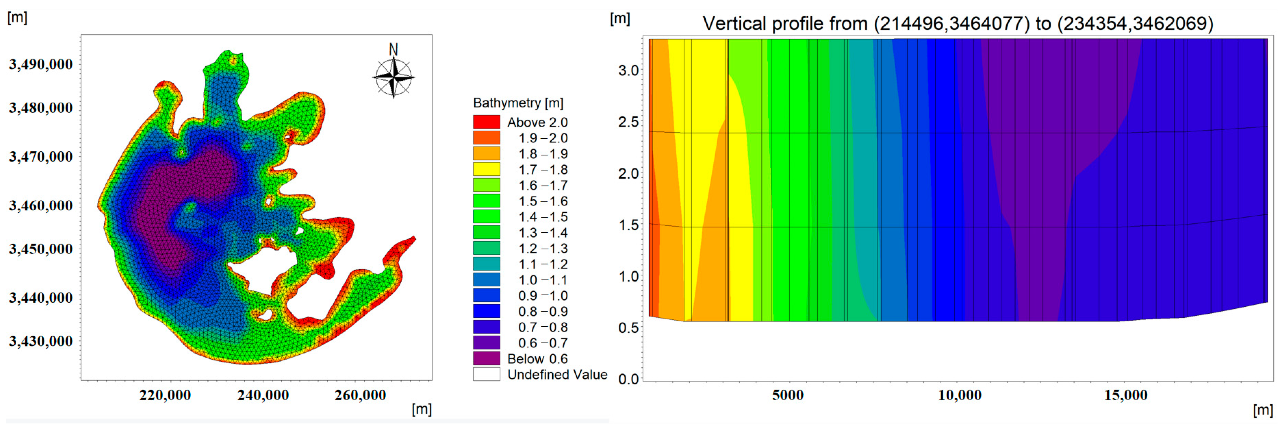
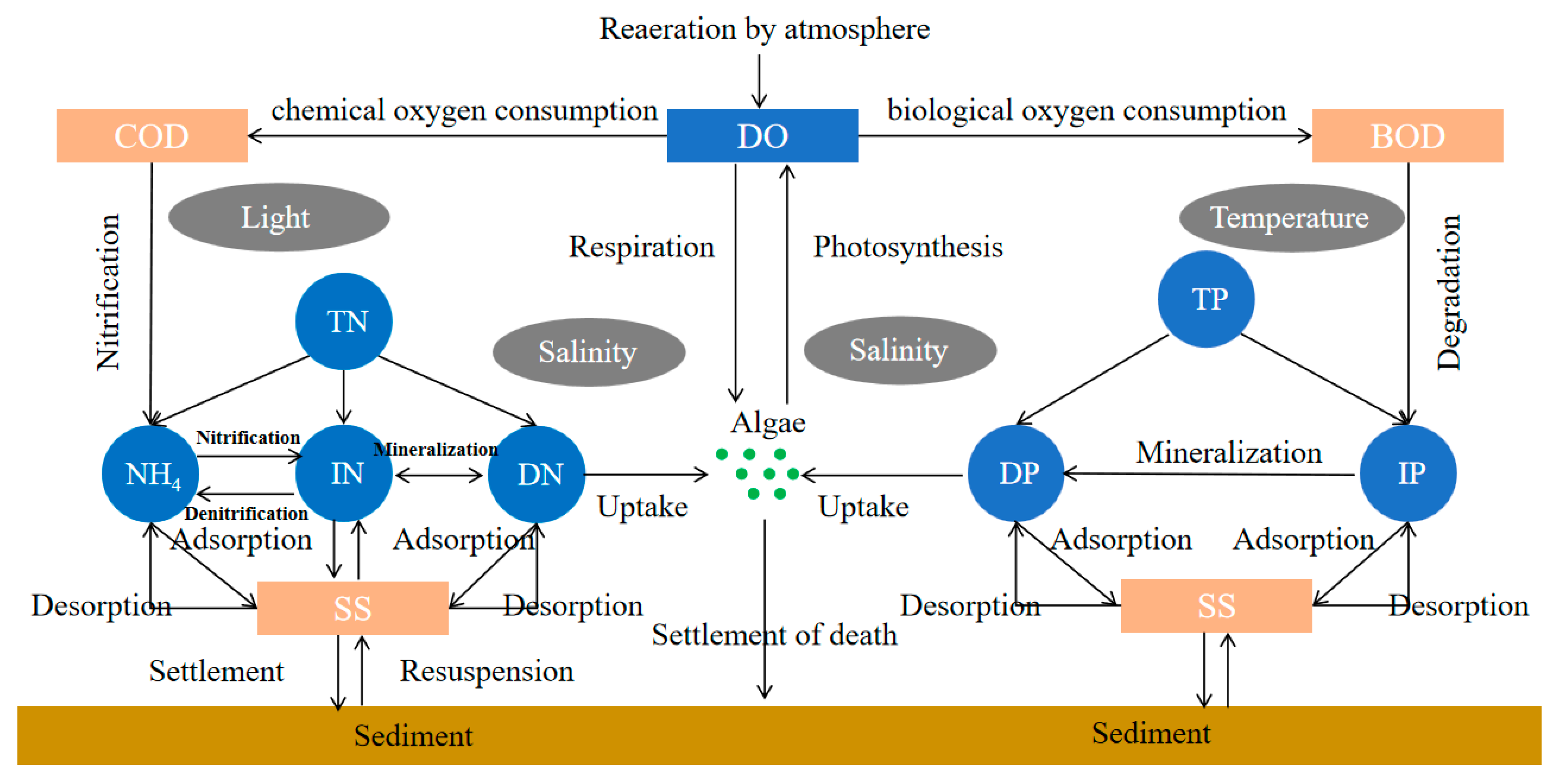
3.2. 3D Water Environment Mathematical Model

Based on SMS and Firebird software (they are the auxiliary software to build the unstructured grid and underwater topography better), unstructured grid division and an underwater topography difference analysis were performed in the Tai Lake area. In this study, the grid spacing was set to 500–800 m, and 5881 unstructured grids were obtained (Figure 3). The measured bottom elevation was measured for the whole lake to obtain the mesh file of the bottom elevation of Tai Lake. The time step was set to 3600 s, and the total calculation time was one year (2017). The calibration and validation monitor stations were in Xidong, Meiliang center, Zhushan center, Dapu, Xiaomei kou, and Xu center. The 3D water environment mathematical model is useful in water quality research [38] and can be created using a hydrodynamic module and an Eco-lab module. The Eco-lab module covers the algae cycle, TN cycle, TP cycle, DO cycle, sediment, light, salinity, and temperature (Figure 4). Here, we chose 39 key parameters, except the system parameters. In this model, the algae cycle included growth, death, uptake, photosynthesis, and respiration; the TN cycle included adsorption, desorption, nitrification, denitrification, and mineralization; the TP cycle included adsorption, desorption, and mineralization; the DO cycle included nitrification, degradation, photosynthesis, and respiration by algae and the atmosphere. TN, TP, and DO could influence the algae directly, therefore, we chose Chl-a, TN, TP, and DO as our indicators.

3.3. Model Performance Assessment

In order to compare the simulated (S) and measured (M) results, we used the root mean square error (RMSE) Equation (1), average relative error (MRE) Equation (2), analysis of correlation coefficient (R²) Equation (3), and the coefficient of Nash model (NSE) Equation (4). The specific formulas are as follows [39]:

$$RMSE=\sqrt{\frac{1}{N}\sum _{i=1}^N{\left(S_i-M_i\right)}^2}$$

(1)

$$MRE=\frac{1}{N}\sum _{i=1}^N\left|S_i-M_i\right|$$

(2)

$$R^2=\frac{{\sum }_{i=1}^N\left(S_i-\overline{S}\right)\left(M_i-\overline{M}\right)}{\sqrt{{\sum }_{i=1}^N{(S_i-\overline{S})}^2{\sum }_{i=1}^N{(M_i-\overline{M})}^2}}$$

(3)

$$NSE=1-\frac{{\sum }_{i=1}^N{(S_i-M_i)}^2}{{\sum }_{i=1}^N{(S_i-\overline{M})}^2}$$

(4)

where N is the total number of simulations, i is the number of simulations, S_i is the value of the ith simulation, M_i is the value of the ith measurement, $\overline{S}$ is the simulated average, and $\overline{M}$ the measured average.

3.4. LHS Uncertainty Analysis Method

Latin hypercube sampling [40] is a optimization method of uncertainty analysis based on the Monte Carlo method. We used the 39-parameter range scale from minimum to maximum as the basic variable value for the uncertainty analysis (Appendix A). Here, the parameter groups were calculated using the LHS method and then, we calculated the different groups with the model, ranking the results and choosing 5% and 95% as the uncertainty boundaries. The specific process is as follows:

Step 1—Parameter grouped Group the input parameters or boundary conditions (m) into equal groups (n groups);

Step 2—Combining sampled Each parameter or boundary condition is randomly sampled in the value range of each different group (n), which is recorded as $x_1, x_2,\dots ,x_m$ and an $m\times n$ matrix is formed after sampling a certain number of parameters according to demand.

Step 3—Model calculated Bring each group of factors into the model for calculation until all factor groups are simulated. Because the model requires a long time for calculation, this study uses 40 central procession unit calculations in parallel, which are performed 25 times in a row and run for a total of 1000 times.

Step 4—Predicted value ranked Sort the n predicted values obtained by simulation according to size.

Step 5—Quantile determinated The cumulative probability assigned to the smallest predicted value is 1/n, the second smallest assigned is 2/n, and so on, until all subsample quantiles are obtained, of which the m input result is m/n × 100%.

Step 6—Uncertain boundary selected Choose 5% and 95% to represent the lower and upper uncertainty boundaries caused by the factor, respectively.

3.5. Morris Sensitivity Analysis Method

The Morris method [41] is a design based on the one-at-a-time (OAT) method, which is suitable for analyzing models with many parameters and a large calculation load. We used the 39-parameter range scale from minimum to maximum as the basic variable value for the sensitivity analysis (Appendix A). Then, we obtained the simulation results from the different parameter groups using the 3D model and calculated the basic influence from Equation (5) as follows:

$$E{E}_i=\frac{f\left(x_1,\cdots ,x_i,\cdots ,x_n\right)-f\left(x\right)}{{\Delta }_i},$$

(5)

where $E{E}_i$ is the basic influence of the ith factor, f(x) represents the initial point of the trajectory, n represents the number of model factors, and ${\Delta }_i$ is the size of the disturbance grid. The sensitivity index (${\mu }_i$) and the interaction between the factors (${\sigma }_i$) can be calculated using Equations (6) and (7), respectively:

$${\mu }_i=\frac{1}{N}\sum _{j=1}^N\left|E{E}_i^j\right|,$$

(6)

$${\sigma }_i=\sqrt{\frac{1}{N-1}{\sum }_{j=1}^N {(E{E}_i^j-\frac{1}{N}{\sum }_{j=1}^{N}E{E}_i^j)}^2},$$

(7)

where $E{E}_i^j$ is the influence result of the ith factor on track j.

4. Results and Discussion

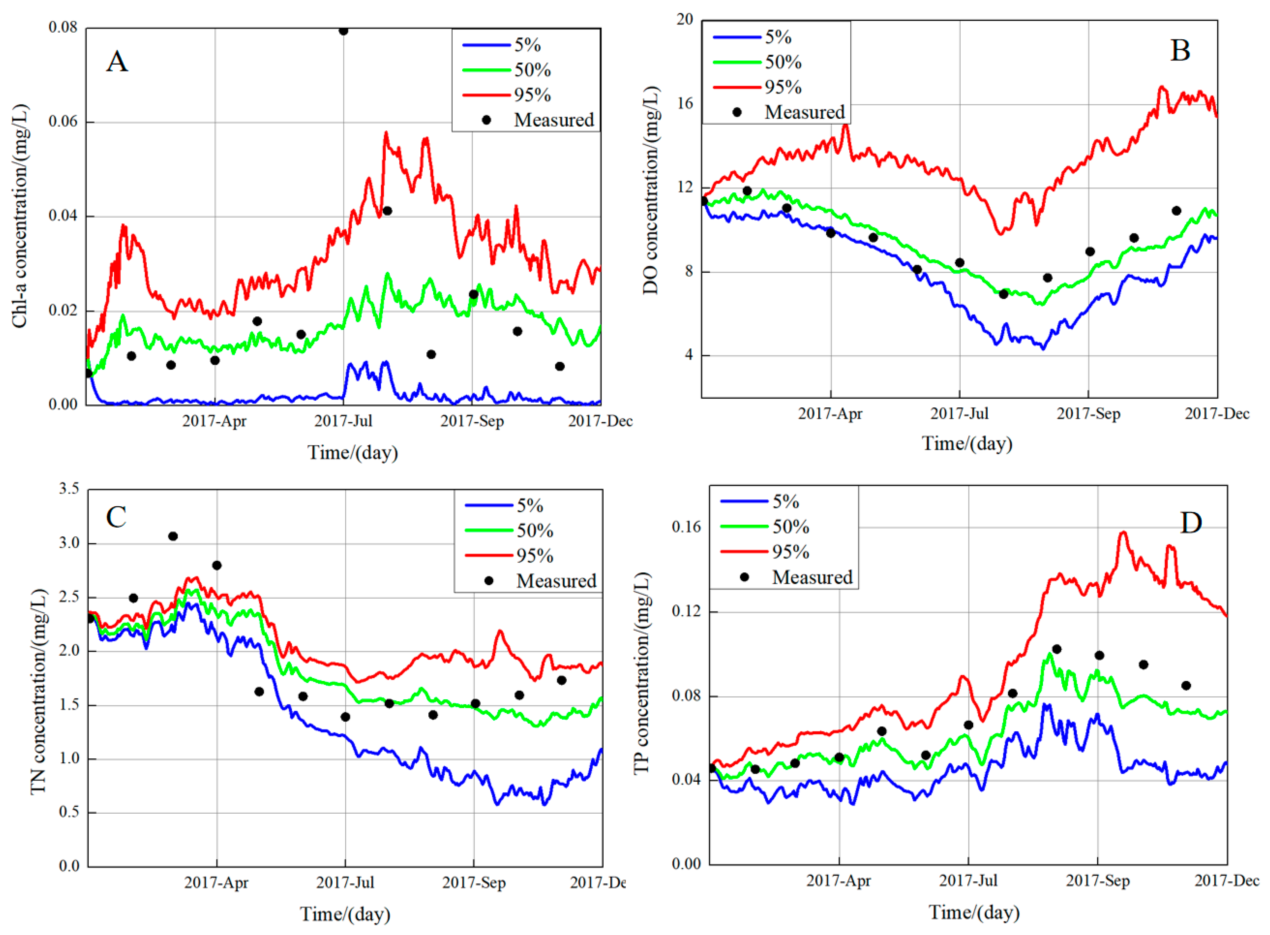
4.1. Calibration and Validation of the 3D Model

When we set the parameter values to those shown in Appendix A, the calibration (January–September, 75 percent) and validation (October–December, 25 percent) results show that the 3D Eco-lab water environment mathematical model has a good simulation effect for Tai Lake (Figure 5). The trend of the simulation curve and the monthly average measured data are basically consistent. Among them, the simulation of Chl-a has a certain deficiency in the peak period of cyanobacteria, which may be related to the absence of a vertical motion module in the model [15], resulting in the lack of a key influencing factor during the cyanobacteria outbreak. However, in general, the results of the simulation of cyanobacteria in other time periods are excellent. The simulation results of dissolved oxygen are basically consistent with the actual monitoring values, and the NSE accuracy is best for this parameter. This is because the dissolved oxygen is mainly affected by temperature and water level, and therefore, the uncertainty is relatively stable [42]. The simulation results of total phosphorus are not very good in the early months, which may be related to the hysteresis, but the simulation results in the later period are very good and are basically consistent with the measured data [43]. The simulation results of total nitrogen also perform very well; only four months were not perfectly captured and the simulated trends and simulated values are highly consistent with the measured data. This proves that TN in Tai Lake is more stable and much easier to treat than TP [36]. In general, the 3D water environment mathematical model simulates Tai Lake well. These parameters have been calibrated in a past paper [44], which helps provide a solid foundation for further uncertainty and sensitivity research.

The 3D water environment mathematical evaluation results show that the simulation errors of water quality and algae in Tai Lake are less than 20% (

Table 2. Model performance assessment depends on different evaluation methods.

Indicators	Time	RMSE	MRE	R2	NSE
TP	Calibration	0.012	0.010	0.945	0.864
	Validation	0.018	0.014	0.921	0.801
TN	Calibration	0.182	0.159	0.956	0.992
	Validation	0.209	0.188	0.915	0.965
Chl-a	Calibration	0.005	0.004	0.865	0.988
	Validation	0.007	0.006	0.831	0.925
DO	Calibration	0.915	0.756	0.901	0.993
	Validation	0.955	0.821	0.869	0.990

), which meets the needs of further simulation research. The RMSE and MRE show the absolute error for the four different indicators. Because they have different value scales, DO will always be greater than the others. Sometimes we use R² and NSE to show the relative error so that we can compare them more easily and clearly. Based on the R² and NSE, the errors of Chl-a and dissolved oxygen are larger than those of TP and TN, indicating that algae and dissolved oxygen are affected by more factors and the internal mechanism [45]. Therefore, further uncertainty and sensitivity research on these characteristics is required in order to identify their specific characteristics and main controlling factors.

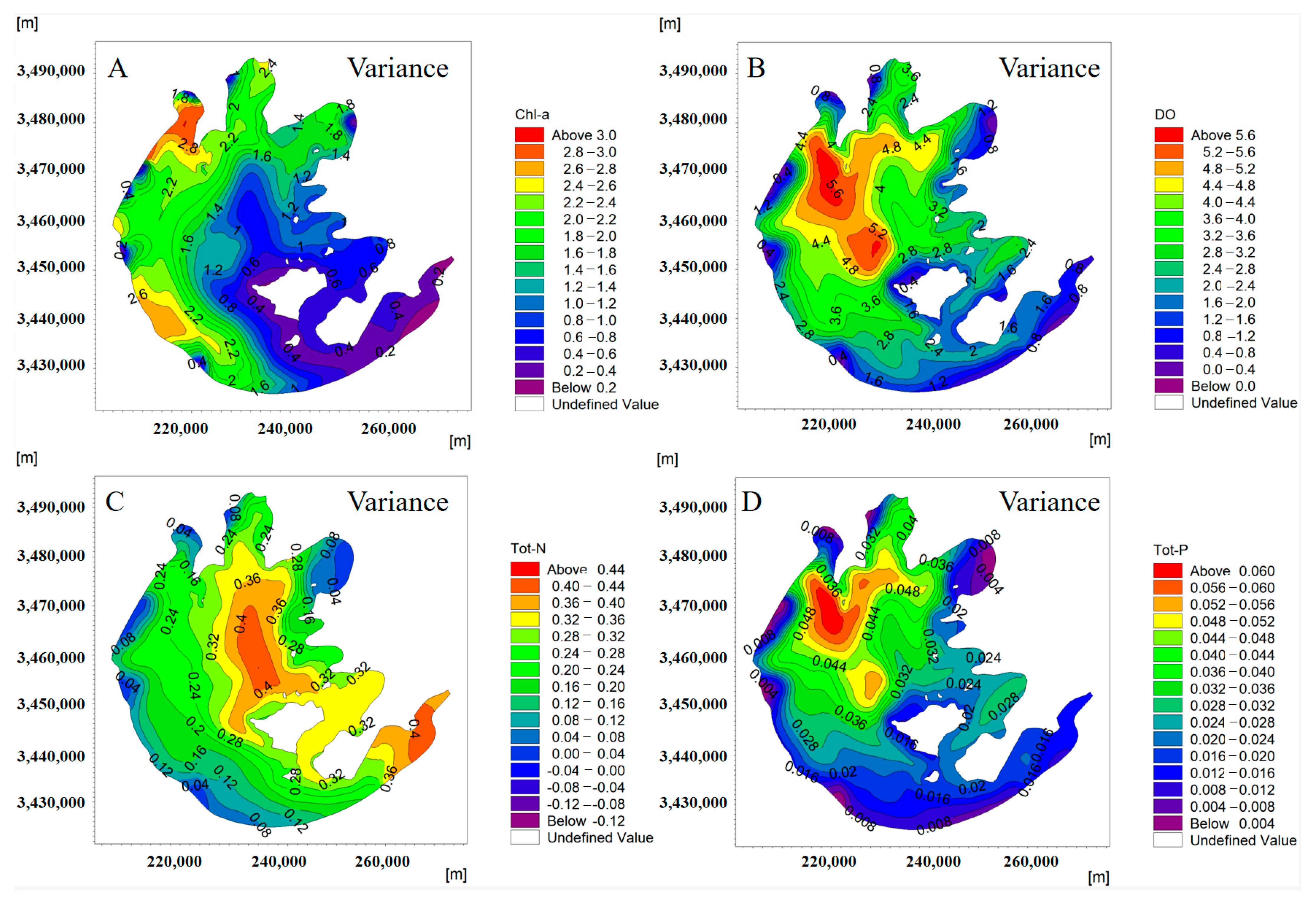
4.2. Spatiotemporal Uncertainty Analysis

Taking the average concentration value of Tai Lake as an example, 1000 groups of samples were obtained based on the LHS method; the uncertainty simulation results of 5%, 50%, and 95% for the four key indicators were obtained in descending order (Figure 6). The results of the long-term series show that the uncertainty of Chl-a in the summer and autumn was significantly greater than that in the spring and winter, which is consistent with the research of Yi et al. [27], which indicated that temperature and light had a decisive effect on cyanobacteria, and also proved that the high temperature and strong light intensity of 2017 (mean annual air temperature was around 16.6 °C) caused the outbreak of cyanobacteria [37]. This study suggests that the water managers who desire ecological stability need to develop methods designed to prevent blooms of cyanobacteria in certain periods when areas have extreme climates at times [46]. The uncertainty related to the DO concentration is inversely proportional to the temperature; the rate of change in DO concentration occurs relatively rapidly and it is minimally affected by other external conditions. The reduction in DO during periods of high temperature also plays a role in promoting outbreaks of cyanobacteria, therefore, this is also a reason why cyanobacteria are prone to undesirable blooms in summer [47]. The uncertainty related to TN and TP was relatively small as compared with that of Chl-a and DO; the level of uncertainty increased after the summer. This may be due to the uncertainty of the model itself [34], which is caused by the long sequence required for the calculation of the model due to it being based on the results of the previous step so that the phenomenon of uncertainty accumulation also appears. This study found an interesting phenomenon, that is, TN is the only indicator with multiple measured values beyond the calculation range of uncertainty, which shows that the external uncertainty of TN is much greater than that of the other indicators.

This study further calculated the spatial uncertainty of the model parameters according to the definition of the variance, and thus, measured the influence of the proportional distribution of the spatial uncertainty of the parameters related to Chl-a, DO, TN, and TP (Figure 7). Among them, the main area of uncertainty for Chl-a was located in the northwestern part of Tai Lake. This was mainly caused by pollutants that mostly enter from the northwestern part of Tai Lake, causing the main concentration of cyanobacteria and nutrients to appear in the northwestern part of Tai Lake [48]. The remaining three indicators’ spatial uncertainties were mainly in the central region, which may be caused by the low elevation of the central region and the surrounding high terrain at the bottom of Tai Lake [49]. However, the specific positions of the occurrence of these three indicators still showed only minor differences. The uncertainty of DO mainly occurred in the most southerly part of Tai Lake, indicating that the uncertainty of DO was not only related to the temperature but also the depth of the water [50]. The location of uncertainty for TN was almost the same as that of DO, which was due to the nitrification of water. Denitrification is closely related to the level of DO of a water body [51]. The 3D Eco-lab model reflects the characteristics of the change in elemental N and O depending on the nitrification and denitrification process well. The uncertainty of TP was mainly concentrated in the eastern lake area, which may be due to the existence and effects of aquatic vegetation in that region [52]. In addition, this study found an interesting result, that is, the main access point to the lake was less affected by the model parameters, which showed that the external conditions play a decisive role in the area near the lake shore. The degree and range of the effect of external conditions on TN were significantly higher than those of the other three indicators, consistent with the previous findings of this study, namely, the uncertainty of external factors on the lake water quality and ecology cannot be completely ignored. Additionally, we can use best management practices (BMPs), i.e., aquatic vegetation restoration, to decrease the heavy pollution area [53] or control the pollution sources from the catchment [54].

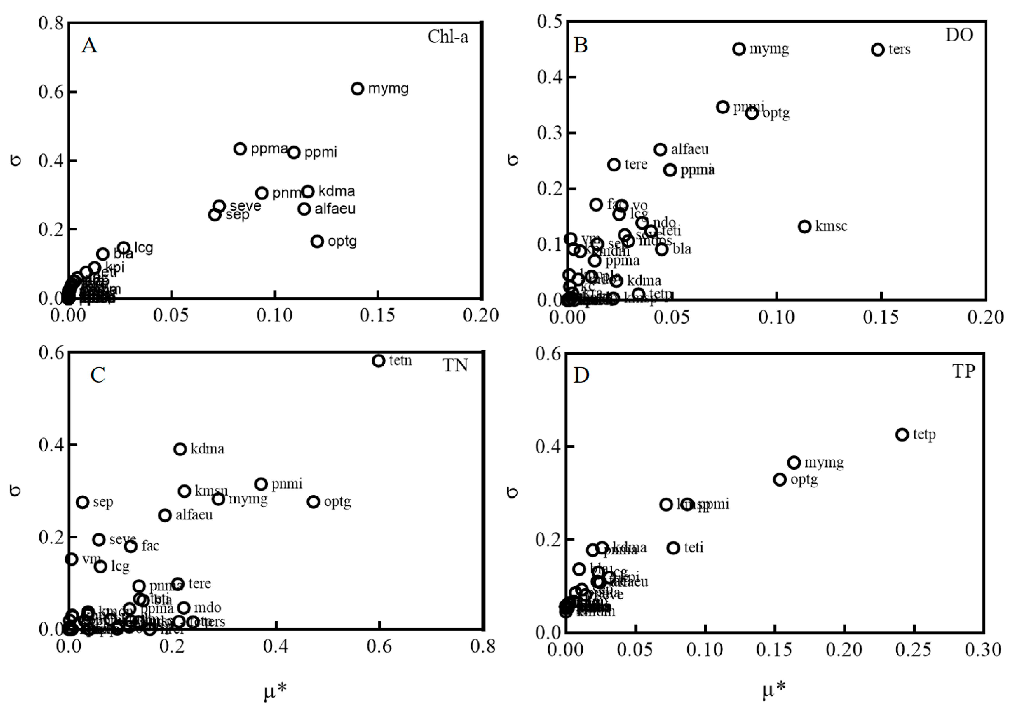
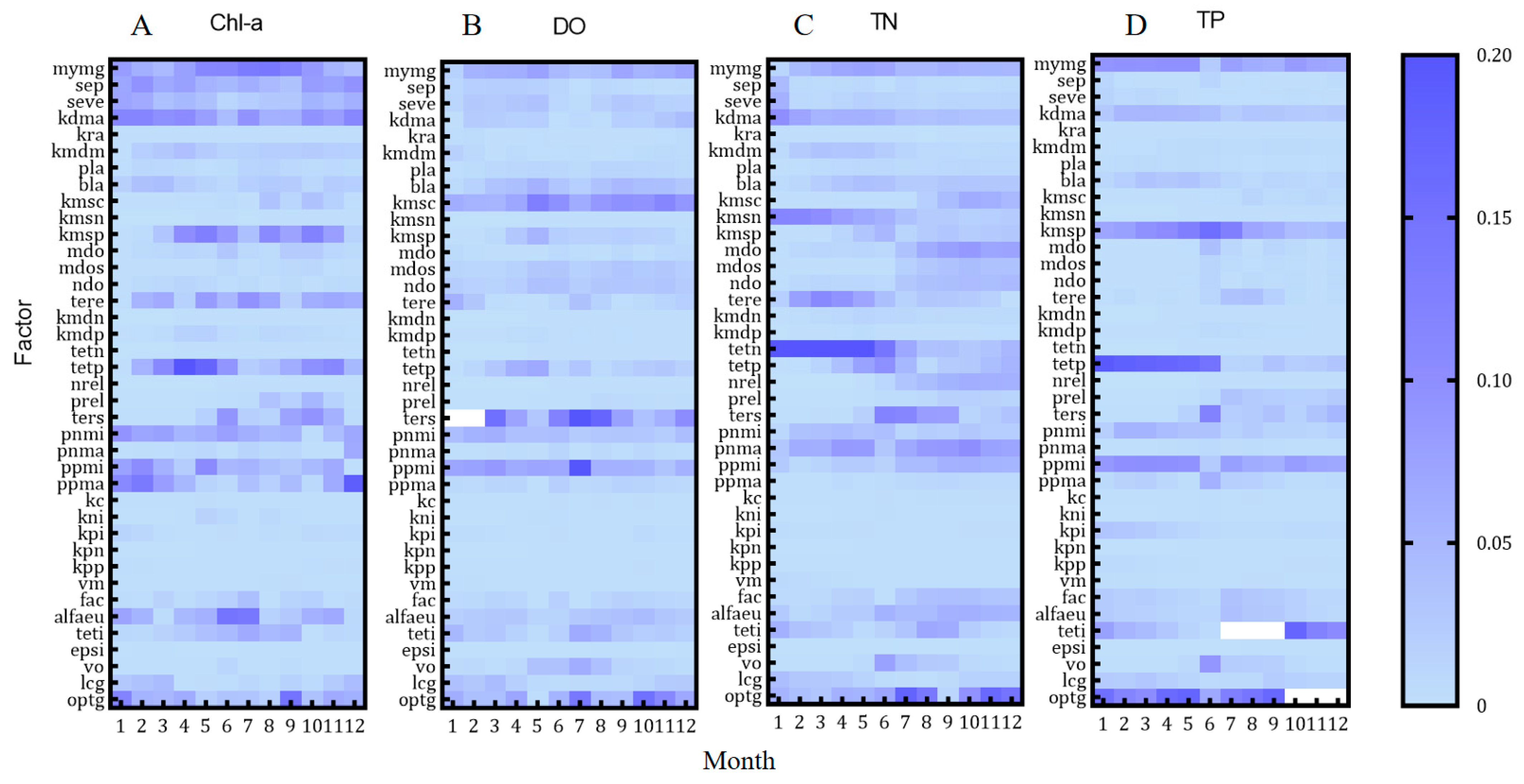
4.3. Sensitivity Analysis at Different Times

In order to more intuitively reflect the sensitivity and correlation of the parameters of each indicator, the Morris index (μ*) and standard deviation (σ) were calculated, which represent the magnitude of parameter sensitivity and correlation, respectively. The six most sensitive of the top 12 parameter factors of the four indicators were mymg, kdma, lcg, pnmi, ppmi, and optg, showing that these parameters are the main control factors in the Eco-lab model (Figure 8).

Among them, the parameter most sensitive to cyanobacteria was mymg. This is the case because Tai Lake is an eutrophic lake, in which almost no nutrient threshold exists [55]; the growth parameter has become the most important parameter affecting the local biomass distribution of cyanobacteria. In addition, the optg, lcg, and alfaeu distributions represent the relationships between cyanobacteria and both temperature and light. Namely, the main control factors for algal blooms are mymg (0.14), optg (0.12), kdma (0.12), alfaeu (0.11) and ppmi (0.11). This is consistent with the findings of Liu et al. (2019) [56]. As we know from the 3D model, algae have a direct relationship with the other three water quality parameters, so all of the key parameters that affect cyanobacteria affect other water quality indicators through transitivity, but the weights may exhibit some differences. For example, mymg and optg have a significant affect on the three other water quality characteristics, but the other control factors are different.

The main factors affecting DO include water temperature, oxygen partial pressure, and respiration [53,57]. The most significant parameters in this study were ters (0.15) and kmsc (0.12), which were different from the main control parameter groups of other indicators. These two main control parameters are related to the respiration of sediment, indicating that the main control factor affecting the DO concentration in the water is the respiration process, not photosynthesis, when the boundary conditions of the model (temperature and air pressure) are determined. For TN and TP, the main parameters were tetn (0.58) and tetp (0.24). This shows that the endogenous release of N and P from sediments with different temperatures plays an important role in Tai Lake [58]. TN and TP were also influenced by mymg (0.3 and 0.17, respectively). Here, we can see synergy between water quality and algal growth, and mymg ranks second in the TP sensitivity analysis results. In the later stage of the management of Tai Lake, certain ecological restoration techniques should be combined to avoid the loss of N and P.

In general, the larger the μ* parameter, the larger the corresponding σ will be (Figure 8), which means that the sensitivity of the parameter is greater, and that the nonlinear form and interaction with other parameters will also be more obvious [59]. This phenomenon leads to the problem of the same effect coming from different parameter groups. Therefore, for similar problems, the model alone cannot fully explain the results.

In order to uncover a deeper temporal law related to the different parameters [60], a further investigation related to the sensitivity of the parameters at different times was conducted (Figure 9). Mymg was found to be the most sensitive parameter to cyanobacteria, which were most active from May to October due to the seasonal (summer and autumn) range of temperatures (20–32 °C), which is very suitable for the growth of cyanobacteria [61,62]. At the same time, the tetn and tetp parameters, which had the most significant impact on TN and TP, played a greater role in the first half of the year, and their sensitivity in the second half of the year decreased significantly. This may be caused by the uncertainty of the model that later caused errors in the calculation of parameter sensitivity. The effect of mymg on TP was obviously higher than that on other indicators except Chl-a, which may be caused by the interaction between cyanobacteria and TP [63,64].

In general, the sensitivity ranking of the four indicators at different times can explain most of the actual phenomena. At the same time, we can also see that the main control parameters during the algal bloom period are growth rate, optimal growth temperature, optimal growth light, and TP uptake rate, which means that the algae outbreak is mainly related to its own growth characteristics, external temperature, external light, and TP concentration [27,65,66]. Thus, we know that algal blooms are related to not only the general water quality but also the climate and different species [67]. In 2017 there was more light, a higher temperature, and a high TP concentration [7], meaning that the algae appeared in the form of large scale blooms in this year.

5. Conclusions

(1)

The 3D water environment mathematical model can play an effective role in water quality simulations of Tai Lake. The simulation accuracy of total phosphorus and total nitrogen is higher than that of Chl-a and dissolved oxygen, and the average error is less than 20%. The 3D Eco-lab model is suitable for research on large shallow lake water quality in other areas.

(2)

The results of the spatiotemporal uncertainty analysis show that Chl-a and TP are closely correlated in Tai Lake, as are TN and DO. This indicates that to prepare for the early warning and prevention of algal blooms, the change in TP concentration in Tai Lake should be monitored closely.

(3)

Based on the meteorological data in 2017, combined with our sensitivity analysis, we conclude that the algal bloom in 2017 is mainly related to the sudden change in climate and the high TP concentration. Therefore, controlling the TP concentration in Tai Lake is still the best method for the Chinese government to solve the problem of algal blooms.

References

- Wei, L.; Zhu, N.; Liu, X.; Zheng, H.; Xiao, K.; Huang, Q.; Liu, H.; Cai, M. Application of Hi-throat/Hi-volume SPE technique in assessing organophosphorus pesticides and their degradation products in surface water from Tai Lake, east China. J. Environ. Manag. 2022, 305, 114346. [Google Scholar] [CrossRef] [PubMed]
- Zhang, H.; Yang, L.; Li, Y.; Wang, C.; Zhang, W.; Wang, L.; Niu, L. Pollution gradients shape the co-occurrence networks and interactions of sedimentary bacterial communities in Taihu Lake, a shallow eutrophic lake. J. Environ. Manag. 2022, 305, 114380. [Google Scholar] [CrossRef] [PubMed]
- Khan, M.Y.A.; Wen, J. Evaluation of physicochemical and heavy metals characteristics in surface water under anthropogenic activities using multivariate statistical methods, Garra River, Ganges Basin, India. Environ. Eng. Res. 2020, 26, 200280. [Google Scholar] [CrossRef]
- Schnedler-Meyer, N.A.; Andersen, T.K.; Hu, F.R.S.; Bolding, K.; Nielsen, A.; Trolle, D. Water Ecosystems Tool (WET) 0.1.0—A new generation of flexible aquatic ecosystem model. Geosci. Model Dev. 2022, 1–24. [Google Scholar] [CrossRef]
- Ghobadi, A.; Cheraghi, M.; Sobhanardakani, S.; Lorestani, B.; Merrikhpour, H. Groundwater quality modeling using a novel hybrid data-intelligence model based on gray wolf optimization algorithm and multi-layer perceptron artificial neural network: A case study in Asadabad Plain, Hamedan, Iran. Environ. Sci. Pollut. Res. 2022, 29, 8716–8730. [Google Scholar] [CrossRef] [PubMed]
- Zou, R.; Wu, Z.; Zhao, L.; Elser, J.J.; Yu, Y.; Chen, Y.; Liu, Y. Seasonal algal blooms support sediment release of phosphorus via positive feedback in a eutrophic lake: Insights from a nutrient flux tracking modeling. Ecol. Model. 2020, 416, 108881. [Google Scholar] [CrossRef]
- Xu, R.; Pang, Y.; Hu, Z. Sensitivity analysis of external conditions based on the MARS-Sobol method: Case study of Tai Lake, China. Water Supply 2021, 21, 723–735. [Google Scholar] [CrossRef]
- Xia, W.; Shoemaker, C.; Akhtar, T.; Nguyen, M.-T. Efficient parallel surrogate optimization algorithm and framework with application to parameter calibration of computationally expensive three-dimensional hydrodynamic lake PDE models. Environ. Model. Softw. 2021, 135, 104910. [Google Scholar] [CrossRef]
- Nielsen, A.; Schmidt Hu, F.R.; Schnedler-Meyer, N.A.; Bolding, K.; Andersen, T.K.; Trolle, D. Introducing QWET—A QGIS-plugin for application, evaluation and experimentation with the WET model. Environ. Model. Softw. 2021, 135, 104886. [Google Scholar] [CrossRef]
- Chou, Q.; Nielsen, A.; Andersen, T.K.; Hu, F.; Chen, W.; Cao, T.; Ni, L.; Søndergaard, M.; Johansson, L.S.; Jeppesen, E.; et al. The impacts of extreme climate on summer-stratified temperate lakes: Lake Søholm, Denmark, as an example. Hydrobiologia 2021, 848, 3521–3537. [Google Scholar] [CrossRef]
- Janssen, A.B.G.; Teurlincx, S.; Beusen, A.H.W.; Huijbregts, M.A.J.; Rost, J.; Schipper, A.M.; Seelen, L.M.S.; Mooij, W.M.; Janse, J.H. PCLake+: A process-based ecological model to assess the trophic state of stratified and non-stratified freshwater lakes worldwide. Ecol. Model. 2019, 396, 23–32. [Google Scholar] [CrossRef]
- Wei, Y.; Yuanxi, L.; Yu, L.; Mingxiang, X.; Liping, Z.; Qiuliang, D. Impacts of rainfall intensity and urbanization on water environment of urban lakes. Ecohydrol. Hydrobiol. 2020, 20, 513–524. [Google Scholar] [CrossRef]
- Li, D.; Hu, L.; Peng, X.; Xiao, N.; Zhao, H.; Liu, G.; Liu, H.; Li, K.; Ai, B.; Xia, H.; et al. A proposed artificial intelligence workflow to address application challenges leveraged on algorithm uncertainty. iScience 2022, 25, 103961. [Google Scholar] [CrossRef]
- Andersen, T.K.; Bolding, K.; Nielsen, A.; Bruggeman, J.; Jeppesen, E.; Trolle, D. How morphology shapes the parameter sensitivity of lake ecosystem models. Environ. Model. Softw. 2021, 136, 104945. [Google Scholar] [CrossRef]
- Wang, Z.; Akbar, S.; Sun, Y.; Gu, L.; Zhang, L.; Lyu, K.; Huang, Y.; Yang, Z. Cyanobacterial dominance and succession: Factors, mechanisms, predictions, and managements. J. Environ. Manag. 2021, 297, 113281. [Google Scholar] [CrossRef]
- Sin, G.; Gernaey, K.V.; Neumann, M.B.; van Loosdrecht, M.C.; Gujer, W. Global sensitivity analysis in wastewater treatment plant model applications: Prioritizing sources of uncertainty. Water Res. 2011, 45, 639–651. [Google Scholar] [CrossRef]
- Zameer, A.; Muneeb, M.; Mirza, S.M.; Raja, M.A.Z. Fractional-order particle swarm based multi-objective PWR core loading pattern optimization. Ann. Nucl. Energy 2020, 135, 106982. [Google Scholar] [CrossRef]
- Jiang, L.; Li, Y.; Zhao, X.; Tillotson, M.R.; Wang, W.; Zhang, S.; Sarpong, L.; Asmaa, Q.; Pan, B. Parameter uncertainty and sensitivity analysis of water quality model in Lake Taihu, China. Ecol. Model. 2018, 375, 1–12. [Google Scholar] [CrossRef]
- Gao, X.; Cui, Y.; Hu, J.; Xu, G.; Wang, Z.; Qu, J.; Wang, H. Parameter extraction of solar cell models using improved shuffled complex evolution algorithm. Energy Convers. Manag. 2018, 157, 460–479. [Google Scholar] [CrossRef]
- Qian, G.; Mahdi, A. Sensitivity analysis methods in the biomedical sciences. Math. Biosci. 2020, 323, 108306. [Google Scholar] [CrossRef]
- Plaas, H.E.; Paerl, H.W. Toxic Cyanobacteria: A Growing Threat to Water and Air Quality. Env. Sci Technol. 2021, 55, 44–64. [Google Scholar] [CrossRef] [PubMed]
- Jordan, M.; Millinger, M.; Thrän, D. Robust bioenergy technologies for the German heat transition: A novel approach combining optimization modeling with Sobol’ sensitivity analysis. Appl. Energy 2020, 262, 114534. [Google Scholar] [CrossRef]
- Liu, W.; Ding, L. Global sensitivity analysis of influential parameters for excavation stability of metro tunnel. Autom. Constr. 2020, 113, 103080. [Google Scholar] [CrossRef]
- Zhou, S.; Guo, X.; Zhang, Q.; Dias, D.; Pan, Q. Influence of a weak layer on the tunnel face stability—Reliability and sensitivity analysis. Comput. Geotech. 2020, 122, 103507. [Google Scholar] [CrossRef]
- Zhang, Q. Global bounded solutions to a Keller–Segel system with singular sensitivity. Appl. Math. Lett. 2020, 107, 106397. [Google Scholar] [CrossRef]
- Li, Y.; Tang, C.; Zhu, J.; Pan, B.; Anim, D.O.; Ji, Y.; Yu, Z.; Acharya, K. Parametric uncertainty and sensitivity analysis of hydrodynamic processes for a large shallow freshwater lake. Hydrol. Sci. J. 2015, 60, 1078–1095. [Google Scholar] [CrossRef]
- Yi, X.; Zou, R.; Guo, H. Global sensitivity analysis of a three-dimensional nutrients-algae dynamic model for a large shallow lake. Ecol. Model. 2016, 327, 74–84. [Google Scholar] [CrossRef]
- Wiltshire, K.H.; Tanner, J.E. Comparing maximum entropy modelling methods to inform aquaculture site selection for novel seaweed species. Ecol. Model. 2020, 429, 109071. [Google Scholar] [CrossRef]
- Dige, N.; Diwekar, U. Efficient sampling algorithm for large-scale optimization under uncertainty problems. Comput. Chem. Eng. 2018, 115, 431–454. [Google Scholar] [CrossRef]
- Shahnewaz, M.; Alam, M.S. Genetic algorithm for predicting shear strength of steel fiber reinforced concrete beam with parameter identification and sensitivity analysis. J. Build. Eng. 2020, 29, 101205. [Google Scholar] [CrossRef]
- King, D.M.; Perera, B.J.C. Morris method of sensitivity analysis applied to assess the importance of input variables on urban water supply yield—A case study. J. Hydrol. 2013, 477, 17–32. [Google Scholar] [CrossRef]
- Cosenza, A.; Mannina, G.; Vanrolleghem, P.A.; Neumann, M.B. Global sensitivity analysis in wastewater applications: A comprehensive comparison of different methods. Environ. Model. Softw. 2013, 49, 40–52. [Google Scholar] [CrossRef]
- Zilverberg, C.J.; Angerer, J.; Williams, J.; Metz, L.J.; Harmoney, K. Sensitivity of diet choices and environmental outcomes to a selective grazing algorithm. Ecol. Model. 2018, 390, 10–22. [Google Scholar] [CrossRef]
- Huang, J.; Gao, J. An improved Ensemble Kalman Filter for optimizing parameters in a coupled phosphorus model for lowland polders in Lake Taihu Basin, China. Ecol. Model. 2017, 357, 14–22. [Google Scholar] [CrossRef]
- Hu, W. A review of the models for Lake Taihu and their application in lake environmental management. Ecol. Model. 2016, 319, 9–20. [Google Scholar] [CrossRef]
- Wang, Y.; Yang, G.; Li, B.; Wang, C.; Su, W. Measuring the zonal responses of nitrogen output to landscape pattern in a flatland with river network: A case study in Taihu Lake Basin, China. Environ. Sci. Pollut. Res. 2022, 29, 34624–34636. [Google Scholar] [CrossRef]
- Guo, J.; Wang, L.; Yang, L.; Deng, J.; Zhao, G.; Guo, X. Spatial-temporal characteristics of nitrogen degradation in typical Rivers of Taihu Lake Basin, China. Sci. Total Environ. 2020, 713, 136456. [Google Scholar] [CrossRef]
- Feng, T.; Wang, C.; Wang, P.; Qian, J.; Wang, X. How physiological and physical processes contribute to the phenology of cyanobacterial blooms in large shallow lakes: A new Euler-Lagrangian coupled model. Water Res. 2018, 140, 34–43. [Google Scholar] [CrossRef]
- Xu, R.; Pang, Y.; Hu, Z.; Kaisam, J.P. Dual-Source Optimization of the “Diverting Water from the Yangtze River to Tai Lake (DWYRTL)” Project Based on the Euler Method. Complexity 2020, 2020, 3256596. [Google Scholar] [CrossRef]
- Sheikholeslami, R.; Razavi, S. Progressive Latin Hypercube Sampling: An efficient approach for robust sampling-based analysis of environmental models. Environ. Model. Softw. 2017, 93, 109–126. [Google Scholar] [CrossRef]
- Ren, J.; Zhang, W.; Yang, J. Morris Sensitivity Analysis for Hydrothermal Coupling Parameters of Embankment Dam: A Case Study. Math. Probl. Eng. 2019, 2019, 2196578. [Google Scholar] [CrossRef] [Green Version]
- Ranjbar, M.H.; Hamilton, D.P.; Etemad-Shahidi, A.; Helfer, F. Individual-based modelling of cyanobacteria blooms: Physical and physiological processes. Sci. Total Environ. 2021, 792, 148418. [Google Scholar] [CrossRef] [PubMed]
- Zhang, S.; Yi, Q.; Buyang, S.; Cui, H.; Zhang, S. Enrichment of bioavailable phosphorus in fine particles when sediment resuspension hinders the ecological restoration of shallow eutrophic lakes. Sci. Total Environ. 2020, 710, 135672. [Google Scholar] [CrossRef]
- Pang, M.; Xu, R.; Hu, Z.; Wang, J.; Wang, Y. Uncertainty and Sensitivity Analysis of Input Conditions in a Large Shallow Lake Based on the Latin Hypercube Sampling and Morris Methods. Water 2021, 13, 1861. [Google Scholar] [CrossRef]
- Cao, H.; Han, L.; Li, L. A deep learning method for cyanobacterial harmful algae blooms prediction in Taihu Lake, China. Harmful Algae 2022, 113, 102189. [Google Scholar] [CrossRef] [PubMed]
- Ke, Z.; Xie, P.; Guo, L. Ecological restoration and factors regulating phytoplankton community in a hypertrophic shallow lake, Lake Taihu, China. Acta Ecol. Sin. 2019, 39, 81–88. [Google Scholar] [CrossRef]
- Xu, D.; Wang, Y.; Liu, D.; Wu, D.; Zou, C.; Chen, Y.; Cai, Y.; Leng, X.; An, S. Spatial heterogeneity of food web structure in a large shallow eutrophic lake (Lake Taihu, China): Implications for eutrophication process and management. J. Freshw. Ecol. 2019, 34, 231–247. [Google Scholar] [CrossRef] [Green Version]
- Xu, H.; Xu, M.; Li, Y. Characterization, origin and aggregation behavior of colloids in eutrophic shallow lake. Water Res. 2018, 142, 11. [Google Scholar] [CrossRef]
- Janssen, A.B.G.; de Jager, V.C.L.; Janse, J.H.; Kong, X.; Liu, S.; Ye, Q.; Mooij, W.M. Spatial identification of critical nutrient loads of large shallow lakes: Implications for Lake Taihu (China). Water Res. 2017, 119, 276–287. [Google Scholar] [CrossRef]
- Hetherington, A.L.; Schneider, R.L.; Rudstam, L.G.; Gal, G.; DeGaetano, A.T.; Walter, M.T. Modeling climate change impacts on the thermal dynamics of polymictic Oneida Lake, New York, United States. Ecol. Model. 2015, 300, 1–11. [Google Scholar] [CrossRef]
- Nizzoli, D.; Welsh, D.T.; Viaroli, P. Denitrification and benthic metabolism in lowland pit lakes: The role of trophic conditions. Sci. Total Environ. 2020, 703, 134804. [Google Scholar] [CrossRef] [PubMed]
- Zhang, T.; Ban, X.; Wang, X. Analysis of nutrient transport and ecological response in Honghu Lake, China by using a mathematical model. Sci. Total Environ. 2017, 575, 418–428. [Google Scholar] [CrossRef] [PubMed]
- Khan, A.; Khan, A.; Khan, F.; Shah, L.; Rauf, A.U.; Badrashi, Y.; Khan, W.; Khan, J. Assessment of the Impacts of Terrestrial Determinants on Surface Water Quality at Multiple Spatial Scales. Pol. J. Environ. Stud. 2021, 30, 2137–2147. [Google Scholar] [CrossRef]
- Khan, A.U.; Jiang, J.; Wang, P.; Zheng, Y. Influence of watershed topographic and socio-economic attributes on the climate sensitivity of global river water quality. Environ. Res. Lett. 2017, 12, 104012. [Google Scholar] [CrossRef] [Green Version]
- Wang, M.; Strokal, M.; Burek, P.; Kroeze, C.; Ma, L.; Janssen, A.B.G. Excess nutrient loads to Lake Taihu: Opportunities for nutrient reduction. Sci. Total Environ. 2019, 664, 865–873. [Google Scholar] [CrossRef]
- Liu, X.; Feng, J.; Wang, Y. Chlorophyll a predictability and relative importance of factors governing lake phytoplankton at different timescales. Sci. Total Environ. 2019, 648, 472–480. [Google Scholar] [CrossRef]
- Terry, J.A.; Sadeghian, A.; Lindenschmidt, K.-E. Modelling Dissolved Oxygen/Sediment Oxygen Demand under Ice in a Shallow Eutrophic Prairie Reservoir. Water 2017, 9, 131. [Google Scholar] [CrossRef] [Green Version]
- Wu, T.; Qin, B.; Brookes, J.D.; Yan, W.; Ji, X.; Feng, J. Spatial distribution of sediment nitrogen and phosphorus in Lake Taihu from a hydrodynamics-induced transport perspective. Sci. Total Environ. 2019, 650, 1554–1565. [Google Scholar] [CrossRef]
- Wang, C.; Peng, M.; Xia, G. Sensitivity analysis based on Morris method of passive system performance under ocean conditions. Ann. Nucl. Energy 2020, 137, 107067. [Google Scholar] [CrossRef]
- Khan, A.; Jiang, J.; Sharma, A.; Wang, P.; Khan, J. How Do Terrestrial Determinants Impact the Response of Water Quality to Climate Drivers?—An Elasticity Perspective on the Water–Land–Climate Nexus. Sustainability 2017, 9, 2118. [Google Scholar] [CrossRef] [Green Version]
- Deng, J.; Paerl, H.W.; Qin, B.; Zhang, Y.; Zhu, G.; Jeppesen, E.; Cai, Y.; Xu, H. Climatically-modulated decline in wind speed may strongly affect eutrophication in shallow lakes. Sci. Total Environ. 2018, 645, 1361–1370. [Google Scholar] [CrossRef] [PubMed]
- Deng, Y.; Zhang, Y.; Li, D.; Shi, K.; Zhang, Y. Temporal and Spatial Dynamics of Phytoplankton Primary Production in Lake Taihu Derived from MODIS Data. Remote Sens. 2017, 9, 195. [Google Scholar] [CrossRef]
- Chao, J.Y.; Zhang, Y.M.; Kong, M.; Zhuang, W.; Wang, L.M.; Shao, K.Q.; Gao, G. Long-term moderate wind induced sediment resuspension meeting phosphorus demand of phytoplankton in the large shallow eutrophic Lake Taihu. PLoS ONE 2017, 12, e0173477. [Google Scholar] [CrossRef] [PubMed]
- Liang, Z.; Chen, H.; Wu, S.; Zhang, X.; Yu, Y.; Liu, Y. Exploring Dynamics of the Chlorophyll alpha-Total Phosphorus Relationship at the Lake-Specific Scale: A Bayesian Hierarchical Model. Water Air Soil Pollut. 2018, 229, 21. [Google Scholar] [CrossRef]
- Wang, J.; Li, X.; Lu, L.; Fang, F. Parameter sensitivity analysis of crop growth models based on the extended Fourier Amplitude Sensitivity Test method. Environ. Model. Softw. 2013, 48, 171–182. [Google Scholar] [CrossRef]
- Liang, H.; Gao, S.; Hu, K. Global sensitivity and uncertainty analysis of the dynamic simulation of crop N uptake by using various N dilution curve approaches. Eur. J. Agron. 2020, 116, 126044. [Google Scholar] [CrossRef]
- Khan, M.Y.A.; ElKashouty, M.; Bob, M. Impact of rapid urbanization and tourism on the groundwater quality in Al Madinah city, Saudi Arabia: A monitoring and modeling approach. Arab. J. Geosci. 2020, 13, 922. [Google Scholar] [CrossRef]