Development and Comparison of Prediction Models for Sanitary Sewer Pipes Condition Assessment Using Multinomial Logistic Regression and Artificial Neural Network

Abstract

Sanitary sewer pipes infrastructure system being in good condition is essential for providing safe conveyance of the wastewater from homes, businesses, and industries to the wastewater treatment plants. For sanitary sewer pipes to deliver the wastewater to the treatment plants, they must be in good condition. Most of the water utilities have aged sanitary sewer pipes. Water utilities inspect sewer pipes to decide which segments of the sanitary sewer pipes need rehabilitation or replacement. The process of inspecting the sewer pipes is described as condition assessment. This condition assessment process is costly and necessitates developing a model that predicts the condition rating of sanitary sewer pipes. The objective of this study is to develop Multinomial Logistic Regression (MLR) and Artificial Neural Network (ANN) models to predict sanitary sewer pipes condition rating using inspection and condition assessment data. MLR and ANN models are developed from the City of Dallas’s data. The MLR model is built using 80% of randomly selected data and validated using the remaining 20% of data. The ANN model is trained, validated, and tested. The significant physical factors influencing sanitary pipes condition rating include diameter, age, pipe material, and length. Soil type is the environmental factor that influences sanitary sewer pipes condition rating. The accuracy of the performance of the MLR and ANN is found to be 75% and 85%, respectively. This study contributes to the body of knowledge by developing models to predict sanitary sewer pipes condition rating that enables policymakers and sanitary sewer utilities managers to prioritize the sanitary sewer pipes to be rehabilitated and/or replaced.

1. Introduction

The provision of wastewater services to communities and municipalities is essential for public health, safety, and socioeconomic development. This requires wastewater infrastructure systems that collect wastewater from homes, businesses, and industry and convey the sewer to the treatment plants. The components of wastewater infrastructure systems include service laterals, sewer pipelines, manholes, force mains, siphons, combined sewer overflow regulations, pumping stations, and wet wells [1,2,3].

According to the [4], wastewater infrastructure was given a D+ score. It is unpredictable to know where or when an accidental pipeline failure would occur. Consequently, and to mitigate this, regulating agencies demand that wastewater collection systems conduct periodic sewer inspections to comply with legal requirements. Due to limited budgets, however, not all segments of sewer pipes in wastewater collections systems can be inspected and assessed. To address this shortcoming of assessing criticality of the sewer pipes, utilities need pipe condition estimation models [5].

With limited budgets, policy makers and utility managers must make rational decisions in replacing and/or rehabilitating the pipelines. Asset managers need to make decisions regarding the selection of optimal rehabilitation action for each sewer condition [6]. Managing these assets rationally is, therefore, fundamental for the sustainability of the services and to the economy of societies [7]. To be able to make effective decisions, most water utilities are implementing asset management. This involves mapping and condition assessment of the wastewater collection systems. In reviewing the sustainability of urban water systems [8], it was concluded that identifying and implementing sustainable rehabilitation interventions in the long-term is essential for the survival of a high-service level urban water system.

2. Literature Review

2.1. Sewer Pipe Classification

Sewer pipes are classified based on several attributes. These include physical and environmental factors.

2.2. Physical Factors

The physical factors include pipe material, diameter, age, length, depth, and slope. Cement-based pipes, vitrified clay pipe (VCP), plastic pipes, and metallic pipes are four categories of pipe material. Ref. [9] discussed types of these pipe categories as: Cement based pipes including concrete pipes and asbestos-cement (AC) pipe. Concrete pipes are nonreinforced concrete pipe (CP), reinforced concrete pipe (RCP), prestressed concrete cylinder pipe (PCCP), reinforced concrete cylinder pipe, bar-wrapped steel-cylinder concrete pipe, and polymer concrete pipe (PCP). The plastic pipes are polyvinyl chloride (PVC) pipe, polyethylene (PE) pipe, glass reinforced pipe (GRP or Fiberglass Pipe). Metallic pipes are ductile iron (DI) pipe and steel pipe. Ref. [10] found that material characteristic has the greatest impact on the pipe condition.

Sewer pipe diameter is a significant variable in pipe condition rating. Most water collection systems use a minimum of 6 in. sewer pipes while a few others use a minimum of 8 in. These two common sizes notwithstanding, pipes can be greater than 96 in. Pipe diameter is one of the factors affecting deterioration of sewer pipes. Ref. [11] stated that some condition prediction models identified that sewer deterioration rate decreases with increasing diameter. “With occurrence of obstacles in the conduit, segments with small diameters are more likely to experience a hydraulic performance drop than large diameter ones” [12].

Pipe age is one of the pipe characteristics that is a significant variable in sewer pipes condition rating. Refs. [12,13] found that pipe age was a significant parameter in the sewer systems deterioration model. Ref. [10] stated that age has a negative impact on pipe condition. Ref. [14] established that the pipe age influenced sewer pipe condition and found that poor pipe sewer condition is higher for pipes more than 50 years. “Most of the condition prediction models developed in previous studies show that pipe age has a significant relationship with deterioration of sewer pipes” [15].

Sewer pipe length is a segment of a pipe that is measured from manhole-to-manhole. Ref. [16] noted that length is relevant in describing sewer deterioration even though it is secondary to pipe material. “Typically, longer manhole-to-manhole sewer pipe segments have higher deterioration rates because the probability of defects is greater in longer pipes” [9]. Ref. [10] established that pipe length is an important factor that influences pipe condition.

Pipe depth is the distance from ground surface to the top of the installed pipe in the ground. [17] determined that pipes buried in depths between 2 m (6 ft) and 3 m (9 ft) were least connected to poor sewer pipe condition. Ref. [9] stated that shallowly buried pipes are subjected to more defects and higher deterioration rate due to surface load, illegal connections, and tree root intrusion.

Slope is the gradient of pipe installed from one manhole to manhole. Ref. [12] described segment slope in percentage per length of a segment. Slope will determine the velocity of flow in the sewer. Flat slope will encourage deposition of debris inside the pipe. Ref. [14] stated that negative slopes and extremely low slopes lead to debris accumulation and blockages. Ref. [18] found that negative and very low slopes were the most harmful conditions for sewer pipes, whereas steep slope high velocities cause erosion in the pipe walls. Pipe age is one of the pipe characteristics that is a significant variable in the condition rating of sewer pipes.

2.3. Environmental Factors

Environmental factors associated with sewer pipe condition rating include, but are not limited to, surface condition, soil type, soil pH, and corrosivity. Surface condition is the ground surface beneath which a sewer pipe is located. Ref. [9] stated that the location of pipe affects the magnitude of surface loading to which it is subject. The most common types of soil classified as soil texture are sand, loam, clay, and rock. Ref. [19] stated that the type of soil is a factor that affects ground loss and stability of the sewer pipeline. The interaction of the soil with the sewer pipes determines the deterioration of pipes.

2.4. Sewer Pipe Condition Prediction Models

Sewer pipes condition prediction models are utilized to determine the condition of non-inspected pipes. These assist operators of water utilities to develop renewal strategies of the pipes and to forecast the evolution of the condition of the sewer network under different investment strategies.

2.5. Statistical Methods

Statistical models establish relations between known pipe variables and the sewer pipe condition based on the condition assessment inspection data. Statistical models include discriminant analysis, logistic regression, binary regression, exponential regression, and Markov, Gomptiz, and Bayesian. “The model is calibrated using maximum likelihood fitting methods to provide the best match between model predictions and recorded failure data. Goodness of fit between model forecasts and actual observations is then demonstrated by comparison with a blind data set that was not part of the calibration process” [20]. Multiple linear regression analysis allows many observed factors to affect y. The general multiple linear regression model can be written as (Equation (1)):

$$\mathrm{y}={\mathsf{\beta }}_0+{\mathsf{\beta }}_1{\mathrm{x}}_1+{\mathsf{\beta }}_2{\mathrm{x}}_2+{\mathsf{\beta }}_3{\mathrm{x}}_1+\dots +{\mathsf{\beta }}_{\mathrm{k}}{\mathrm{x}}_{\mathrm{k}}+\mathrm{u}$$

(1)

• β₀ is the intercept
• β₁ is the parameter associated with x₁,
• β₂ is the parameter associated with x₂, and so on
• is the parameters that cannot be included and are collectively contained in u

The equation below is a multiple regression where Y is a predicted outcome for individual based on (a) the Y intercept, a, the value of Y when all predictor values are 0, (b) the product of the independent variables, X_s, and the regression coefficients, b_k; and (c) the residual, ε_i (Equations (2)–(5)):

$${\mathrm{Y}}_{\mathrm{i}}=\mathrm{a}+{\mathrm{b}}_1{\mathrm{X}}_1+\dots +{\mathrm{b}}_{\mathrm{k}}{\mathrm{X}}_{\mathrm{k}}+{\mathsf{\epsilon }}_{\mathrm{i}}$$

(2)

Odds and Logit

$$\mathrm{Odds}\left(\mathrm{Y}=1\right)=\frac{\mathrm{P}\left(\mathrm{Y}=1\right)}{1-\mathrm{P}\left(\mathrm{Y}=1\right)}$$

(3)

Log odds

$$\ln \frac{\mathrm{P}\left(\mathrm{Y}=1\right)}{1-\mathrm{P}\left(\mathrm{Y}=1\right)}=\mathrm{Logit}\left(\mathrm{Y}\right)=\mathsf{\alpha }+{\mathsf{\beta }}_1{\mathrm{X}}_1+{\mathsf{\beta }}_2{\mathrm{X}}_2+\dots +{\mathsf{\beta }}_{\mathrm{m}}{\mathrm{X}}_{\mathrm{m}}$$

(4)

Ref. [2] used age, diameter, length, slope, and material, and built a logistic regression model as follows (Equation (5)):

$$\begin{array}{c}{\mathrm{Y}}^{\ast }={\propto }_0+{\mathsf{\beta }}_1\times \mathrm{Age}+{\mathsf{\beta }}_2\times \mathrm{diameter}+{\mathsf{\beta }}_3\times \mathrm{length}+{\mathsf{\beta }}_4\times \mathrm{slope}\\ +{\mathsf{\beta }}_5\times \mathrm{material}+\mathsf{\epsilon }\end{array}$$

(5)

where Y^* is the unobservable conduit condition, α₀ is the threshold, β₁…. β₅ are regressor coefficients.

A logistic model describes the relationship between an outcome (i.e., dependent or response) and a set of prediction (i.e., independent or explanatory) variables, often referred to as covariates [21]. Equation (6) represents logistic regression model according to [3].

$$\log \left[\frac{\mathsf{\pi }}{1-\mathsf{\pi }}\right]\mathrm{Y}=\lfloor \frac{\mathrm{p}\left(\mathrm{y}=1|{\mathrm{x}}_1\dots .{\mathrm{x}}_{\mathrm{n}}\right)}{1-\mathrm{p}\left(\mathrm{y}=1|{\mathrm{x}}_1\dots .{\mathrm{x}}_{\mathrm{n}}\right)}\rfloor =\mathrm{a}+{\mathsf{\beta }}_1{\mathrm{x}}_1+{\mathsf{\beta }}_2{\mathrm{x}}_2\dots ..+{\mathsf{\beta }}_{\mathrm{p}}{\mathrm{x}}_{\mathrm{p}}$$

(6)

where:

• Y = dependent variable
• a = intercept parameter
• β_p = regression coefficients associated with p independent variables.
• Probability of (y = 1) determined using exponential transformation.
• π = $\mathrm{p}\left(\mathrm{y}=1|{\mathrm{x}}_1\dots .{\mathrm{x}}_{\mathrm{n}}\right)$

In this model, new values of Y can be forecasted with new observed values of X.

Equation (7) shows general function of binary logistic regression. π represents Pr (Y = 1) meaning probability associated with outcome of condition 1. Consequently, 1 − π represents Pr (Y = 0) meaning probability of outcome of condition 0. π/(1 − π) means the odds of having (Y = 1).

Multinomial logistic regression is an extension of binary logistic regression and can be used when dependent variable is categorical and has more than two levels [3].

$$\ln \lfloor \frac{\mathrm{Pr}\left(\mathrm{Y}=\mathrm{i}|{\mathrm{x}}_1\dots {\mathrm{x}}_{\mathrm{n}}\right)}{\mathrm{Pr}\left(\mathrm{Y}=\mathrm{k}|{\mathrm{x}}_1\dots {\mathrm{x}}_{\mathrm{n}}\right)}\rfloor ={\mathsf{\beta }}_0+{\mathsf{\beta }}_{\mathrm{i}1}{\mathrm{x}}_1+{\mathsf{\beta }}_{\mathrm{i}2}{\mathrm{x}}_2\dots ..+{\mathsf{\beta }}_{\mathrm{in}}{\mathrm{x}}_{\mathrm{n}}$$

(7)

where,

• i = 1, 2, …, k − 1 correspond to categories of the dependent variable,
• xs are independent variables,
• n is the number of independent variables,
• ${\mathsf{\beta }}_0$ is the intercept for category i,
• ${\mathsf{\beta }}_{\mathrm{is}}$ are the regression coefficients of independent variables defined for each category i.

Assuming three sewer pipe conditions using Equations (8) and (9), Equations (10)–(12) represent multinomial logistic regression for a pipe system with three condition levels 0, 1, and 2. Category zero (0) is used as the reference value. The model is developed with logit functions. To develop the model, p covariate and a constant term were denoted by the vector x [22].

$${\mathrm{g}}_1\left(\mathrm{x}\right)= \ln \lfloor \frac{\mathrm{Pr}\left(\mathrm{Y}=1|\mathrm{x}\right)}{\mathrm{Pr}\left(\mathrm{Y}=0|\mathrm{X}\right)}\rfloor ={\mathsf{\beta }}_{10}+{\mathsf{\beta }}_{11}{\mathrm{x}}_1+{\mathsf{\beta }}_{12}{\mathrm{x}}_2\dots ..+{\mathsf{\beta }}_{1\mathrm{p}}{\mathrm{x}}_{\mathrm{p}}=\mathrm{x}{\prime \mathsf{\beta }}_1$$

(8)

$${\mathrm{g}}_2\left(\mathrm{x}\right)= \ln \lfloor \frac{\mathrm{Pr}\left(\mathrm{y}=2|\mathrm{x}\right)}{\mathrm{Pr}\left(\mathrm{y}=0|\mathrm{X}\right)}\rfloor ={\mathsf{\beta }}_{20}+{\mathsf{\beta }}_{21}{\mathrm{x}}_1+{\mathsf{\beta }}_{22}{\mathrm{x}}_2\dots ..+{\mathsf{\beta }}_{2\mathrm{p}}{\mathrm{x}}_{\mathrm{p}}=\mathrm{x}{\prime \mathsf{\beta }}_2$$

(9)

$$\mathrm{Pr}\left(\mathrm{Y}=0|\mathrm{x}\right)=\frac{1}{1+{\mathrm{e}}^{{\mathrm{g}}_1\left(\mathrm{x}\right)}+{\mathrm{e}}^{{\mathrm{g}}_{2\left(\mathrm{x}\right)\prime }}}$$

(10)

$$\mathrm{Pr}\left(\mathrm{Y}=1|\mathrm{x}\right)=\frac{{\mathrm{e}}^{{\mathrm{g}}_1\left(\mathrm{x}\right)}}{1+{\mathrm{e}}^{{\mathrm{g}}_1\left(\mathrm{x}\right)}+{\mathrm{e}}^{{\mathrm{g}}_{2\left(\mathrm{x}\right)\prime }}}$$

(11)

$$\mathrm{Pr}\left(\mathrm{Y}=2|\mathrm{x}\right)=\frac{{\mathrm{e}}^{{\mathrm{g}}_{2\left(\mathrm{x}\right)}}}{1+{\mathrm{e}}^{{\mathrm{g}}_1\left(\mathrm{x}\right)}+{\mathrm{e}}^{{\mathrm{g}}_{2\left(\mathrm{x}\right)\prime }}}$$

(12)

Using the convention for the binary model, π_j (x) = Pr (Y = j |x) for j = 0, 1, 2.

2.6. Artificial Intelligence System

ANN is one of the modeling techniques of artificial intelligence modeling techniques. According to [23], some emerging techniques for artificial intelligence systems seek to make better use of human reasoning to solve problems involving incomplete knowledge and use of descriptive terms. ANN predicts output from input information in a manner that simulates the operation of the human central nervous system [17]. Ref. [20] stated that ANN is being increasingly used to solve complex problems, which are also often treated as ‘black box’ solutions. Ref. [20] stated that ANN has layers of nodes which provide a functional relationship between input information and predicted output. The layers are trained on historical data sets. These data sets demonstrate the actual relationship between input and output information.

According to Ref. [24], ANN can learn the patterns of the underlying process from past data, capturing the relations between the inputs and the outputs. According to [25], ANN is a set of independent neurons linked together in the same way as the synapses, neurons, and dendrites of our brain [26]. The neural network learns and execute tasks. During training, the network modifies the weights of the links among the neurons in a way that each input produces the expected outputs. The output is the dependent variable, and the inputs are independent variables.

In this study, three-layer feed-forward neural networks with back propagation (BP) learning were constructed for computation of eleven physical and environmental input variables, as shown in Figure 1.

Figure 1 shows the algorithm having nodes and network lines. The lines are assigned weights of the connecting nodes. Equation (13) shows a relationship between the input and output variables:

$${\mathrm{y}}_{\mathrm{t}}={\mathrm{w}}_0+{\displaystyle \sum }_{\mathrm{j}=1}^{\mathrm{q}}{\mathrm{w}}_{\mathrm{j}}·\mathrm{g}\left({\mathrm{w}}_{0\mathrm{j}}+{\displaystyle \sum }_{\mathrm{i}=1}^{\mathrm{p}}{\mathrm{w}}_{\mathrm{ij}}{\mathrm{y}}_{\mathrm{t}-\mathrm{i}}\right)+{\mathsf{\epsilon }}_{\mathrm{t}}$$

(13)

where, w_ij (i = 0, 1, 2,…..p, j = 1, 2……q) and w_j (j = 0, 1, 2,….., q) are model parameters often called connection weights; p is the number of input nodes and q is the number of hidden nodes.

Figure 2 shows a diagram demonstrating input with a summation n feed into a neuron that computes the inputs and produces a binary output, y, which is either +1 or −1. The bias weight, Ɵ, is introduced with a fixed input at +1. The bias weight allows greater flexibility of the learning process.

$$\mathrm{y}=ƒ\left({\displaystyle \sum }_{\mathrm{i}=1}^{\mathrm{n}}{\mathrm{W}}_{\mathrm{i}}{\mathrm{X}}_{\mathrm{i}}\right)={|}_{-1 \mathrm{when} {\displaystyle \sum }_{\mathrm{i}=1}^{\mathrm{n}}{\mathrm{W}}_{\mathrm{i}}{\mathrm{X}}_{\mathrm{i}}\ge 0}^{1 \mathrm{when}{\displaystyle \sum }_{\mathrm{i}=1}^{\mathrm{n}}{\mathrm{W}}_{\mathrm{i}}{\mathrm{X}}_{\mathrm{i}}>0}$$

(14)

In Equation (14), y is the neuron and f is a threshold function known as the neuron’s transfer function, which gives an output of +1 whenever Σwixi is greater than zero (the threshold value) or −1 whenever Σwixi is less than (or equal to) zero [28].

In this study, the activation function used to act upon input to get output is bipolar sigmoid function. The bipolar sigmoid function Formula is in Equation (15) and Figure 3 [30]).

The output of the bipolar sigmoid function is between −1 and 1.

$$\mathrm{ƒ}\left(\mathrm{x}\right)=\frac{1}{1+{\mathrm{e}}^{-\mathsf{\lambda }\mathrm{x}}}-1=\frac{1-{\mathrm{e}}^{-\mathsf{\lambda }\mathrm{x}}}{1+{\mathrm{e}}^{-\mathsf{\lambda }\mathrm{x}}}$$

(15)

2.7. Problem Statement and Objectives

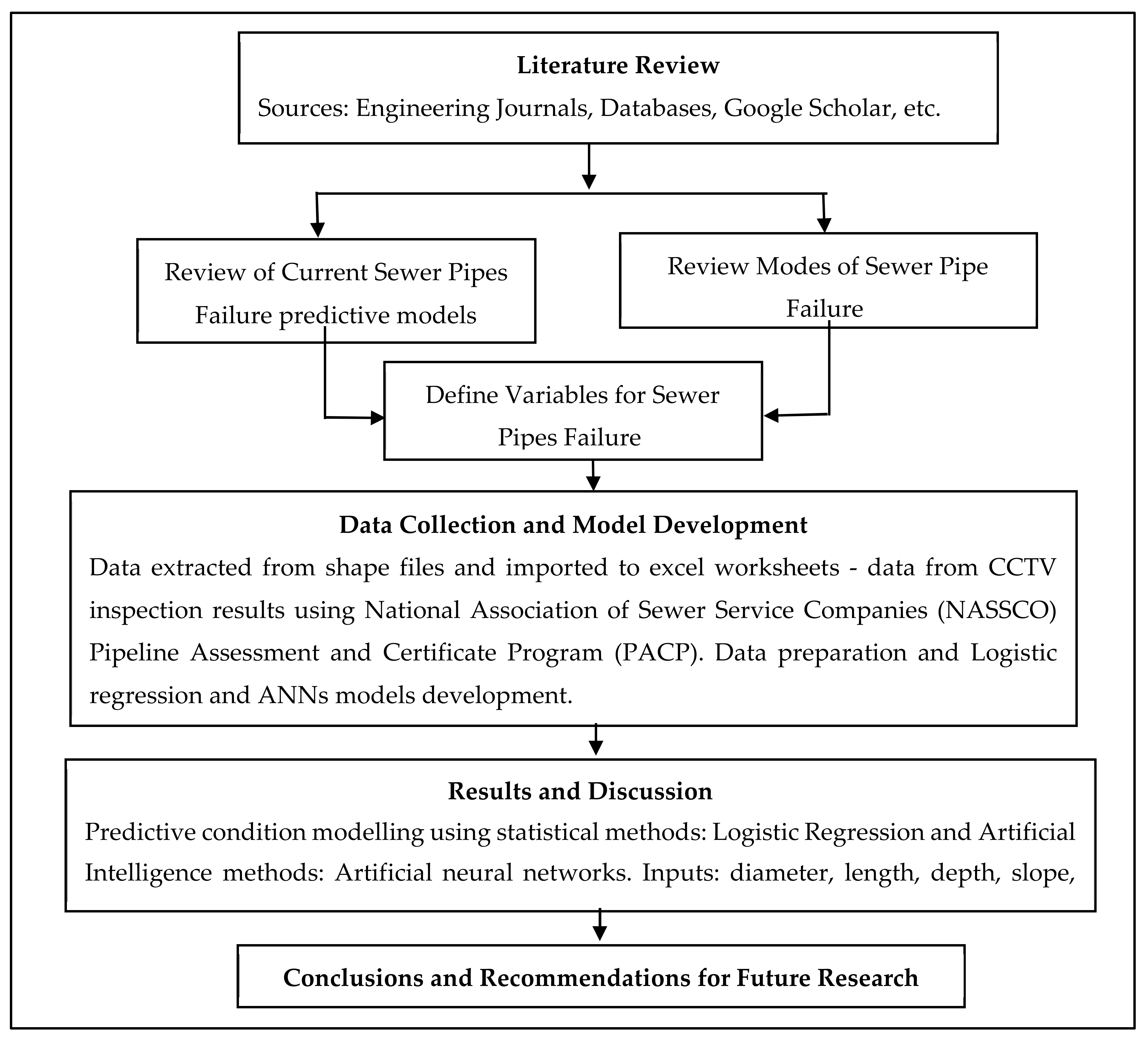
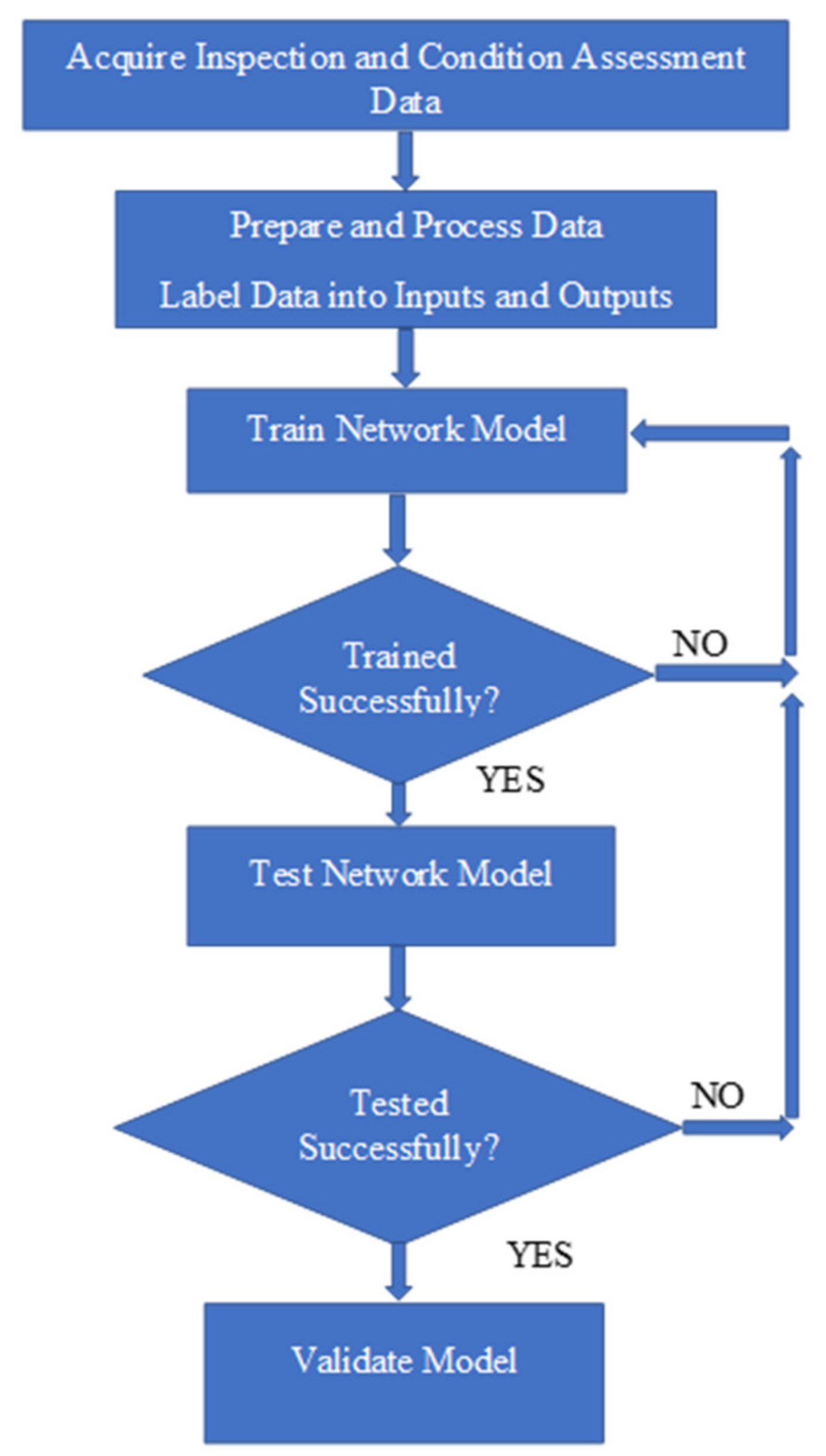
Ref. [1] stated that more investigation is required to identify the influence of physical and environmental factors that affect deterioration of sewer pipes. Additionally, they recommended future research to investigate more pipe material such as steel and concrete pipes in sewer networks and compare the results, and that results of prediction models should be developed for different cities. Ref. [31] review on sewer pipes condition prediction models observed that there is a need for more research to predict condition of sewer pipes with higher accuracy and confidence level.

Following his research on advanced sewer asset management using dynamic deterioration models, Ref. [32] discovered there was still room for improvement. Accordingly, he recommended, in future research, a more comprehensive model be developed by incorporating additional location related attributes such as soil type, water table, among others. In a later study, Ref. [17] advised municipalities to develop and implement risk assessment models for their utilities to get the best utility of their limited budgets available for replacing deteriorating assets. Ref. [33], in their research on infrastructure management and deterioration risk assessment of wastewater collection systems, advised that the deterioration models can be improved by addition or consideration of other independent variables such as soil type, groundwater level, and initial quality of construction. Ref. [33] recommended environmental factors, including surface condition, soil type, corrosivity concrete, corrosivity steel, and pH considered in building the models were included in this dissertation. Ref. [13] recommended factors like type of soil backfill, H₂S, and groundwater level to be investigated to understand sewer deterioration mechanism and develop an effective model. Surface condition and corrosivity variables have not been studied more by others.

According to [16], the improvement of technical asset management and the use of digital solutions to improve the efficiency of inspection and rehabilitation strategies is the promising leverage of utilities. Ref. [16] further stated that most metrics are based on statistics and do not provide understanding of deteriorations for sewer operators. Accordingly, there is a need to utilize artificial intelligence methods and compare the results to those of statistical methods.

The objective of this research is to develop MLR and ANN models to predict sanitary sewer pipes condition rating using inspection and condition assessment data. The secondary objectives of this research are to identify, evaluate, categorize, and develop relationships of different factors affecting sewer pipes condition ratings and to compare the performance of MLR and ANN for predicting sewer pipes condition. The adopted methodology is explained as follows.

3. Methodology

Figure 4 illustrates the methodology adopted to carry out this research. First, utilizing engineering journals, databases, and Google Scholar, a thorough literature review was conducted to mainly study current sewer pipe predictive models, modes of sewer pipe failure, and variables for sewer pipe failure.

In addition to physical, environmental, and operational factors influencing sewer pipes failure, literature on the failure of sewer pipe and risk process evaluation were reviewed. Second, data were collected from Geographical Information System (GIS) shape files for the City of Dallas Water Utilities (DWU) GIS web/database. The GIS data originated from condition assessment and CCTV inspection records.

The data comprised of pipe segments/locations, length (manhole to manhole), pipe material, pipe diameter, pipe age (current year minus year of installation), depth (depth of backfill over the crown of pipe in ft), soil conditions, corrosivity, slope, surface condition–highway/street, and PACP condition rating. Third, the data were prepared, processed, and analyzed. Condition rating was designated as the dependent variable, while physical and environmental factors were independent variables.

4. Model Development

In this section, multinomial logistic regression and neural networks model development are illustrated. The development of the models involved a multinomial logistic regression model that was developed using IBM SPSS Statistics (version 27). ANN model was developed using Brain maker California Scientific Software. Before the development of the models, eighty percent (80%) of the data were randomly selected and the remaining 20% was set aside to validate the models and/or used as a case study to check the applicability of the models. Eighty-five percent (85%) and fifteen percent (15%) of the randomly selected 80% data were used in developing and testing the ANN model, respectively.

Table 1. Sample of 80% of Sewer Pipes Dataset.

ID	Diameter	Age	Pipe Material	Slope	Surface Condition	Depth	Length	pH	Soil Type	Corrosion Concrete	Corrosion Steel	Condition Rating
2472	12	43	PVC	0.24	Street	15	480.157	6.7	Sand	Low	Moderate	1
1814	10	50	VCP	0.1	Easement	15	421.0372	6.7	Sand	Low	Moderate	1
843	6	97	VCP	0.8	Alley	15	263.5681	6.7	Sand	Low	Moderate	1
2343	8	23	PVC	0.3	Street	15	235.9731	6.7	Sand	Low	Moderate	1
2795	18	50	VCP	0.08	Alley	15	80.58689	6.7	Sand	Low	Moderate	1
65	8	50	VCP	0.3	Street	11	535.9586	6.7	Sand	Low	Moderate	1
623	12	71	CONC	0.6	Highway	10	472.1441	6.7	Sand	Low	Moderate	1
624	24	64	CONC	0.12	Street	10	465.4685	6.7	Sand	Low	Moderate	1
2366	12	51	VCP	0.3	Alley	10	401.3963	6.7	Sand	Low	Moderate	1
3215	8	22	PVC	0.33	Street	10	384.402	6.7	Sand	Low	Moderate	1
3097	12	51	VCP	0.3	Street	10	325.2434	6.7	Sand	Low	Moderate	1
1365	8	24	PVC	0.4	Alley	10	283.7502	6.7	Sand	Low	Moderate	1
3327	48	29	PVC	0.14	Street	10	278.4683	6.7	Sand	Low	Moderate	1
2146	12	39	PVC	2.1	Street	10	159.0316	6.7	Sand	Low	Moderate	1
2295	15	66	VCP	0.32	Street	10	156.1034	6.7	Sand	Low	Moderate	1
285	8	35	PVC	0.8	Easement	10	99.28742	6.7	Sand	Low	Moderate	1
181	10	48	VCP	0.8	Alley	10	70.07311	6.7	Sand	Low	Moderate	1
47	8	16	PVC	0.4	Street	10	24.48685	6.7	Sand	Low	Moderate	1
2428	12	9	PVC	0.2	Street	8	479.9761	6.7	Sand	Low	Moderate	1

shows a sample of the 80% sewer pipes dataset.

4.1. Multinomial Logistic Regression Model

Multinomial logistic regression analysis evaluated the relationship between eleven (11) independent or predictor variables and one (1) dependent variable. Pipe material, diameter, age, slope, depth, surface condition, soil type, corrosivity concrete, corrosivity steel, and pH were independent variables used to generate prediction models. The condition rating score was the dependent variable.

4.1.1. Model Parameters Estimation

The data were randomly divided into 80% and 20% for multinomial logistic regression model development and validation, respectively. MLR analysis was conducted, and 4 models were built based on sewer pipes condition ratings 1, 2, 3, and 4. Condition 5 was used as the reference category. Table 1 shows a sample of 80% of the sewer pipes dataset.

4.1.2. Validation of Multinomial Logistic Model

Model parameters estimation tables were used to derive one set of model equation broken down into four multinomial logistic regression equations, one for each condition category relative to reference category for sewer pipe condition 5. The four equations were used to predict sewer pipe conditions 1, 2, 3, and 4, relative to sewer pipes condition 5 that was used as a reference category. The variables coefficients (β) were used to develop the 4 multinomial logistic regression equations relative to condition 5 (C = 5) reference category. The equations are presented in Equations (16)–(19).

$$\begin{array}{l}{\mathrm{g}}_1\left(\mathrm{x}\right)= \ln \left[\frac{\mathrm{Pr}\left(\mathrm{C}=1\right)}{\mathrm{Pr}\left(\mathrm{C}=5\right)}\right]\\ =0.978\ast \mathrm{Diameter}+0.945\ast \mathrm{Age}+1.023\ast \mathrm{Slope}+1.018\ast \mathrm{Depth}+0.999\ast \mathrm{Length}\\ +1.321\ast \mathrm{pH}+1.146\ast \mathrm{MaterialCONC}+1.899\ast \mathrm{MaterialPVC}+0.721\ast \mathrm{SurfaceAlley}\\ +0.771\ast \mathrm{SurfaceEasement}+0.879\ast \mathrm{SurfaceHighway}+0.619\ast \mathrm{SoilTypeClay}+1.037\\ \ast \mathrm{SoilTypeLoam}+0.942\ast \mathrm{SoilTypeRock}+0.962\ast \mathrm{CorrosivityConcreteHigh}+3.653\\ \ast \mathrm{CorrosivityConcreteLow}+1.533\ast \mathrm{CorrosivitySteelHigh}\end{array}$$

(16)

where:

• Pr (C = 1) is the probability of sanitary sewer pipe condition dependent variable being condition 1 relative to condition 5.
• Pr (C = 5) is the probability of reference category condition 5.

Diameter, Age, Slope, Depth, Length, Material, Surface, Soil Type, and Corrosivity are independent variables that influence sanitary sewer pipe condition.

$$\begin{array}{l}{\mathrm{g}}_2\left(\mathrm{x}\right)= \ln \left[\frac{\mathrm{Pr}\left(\mathrm{C}=2\right)}{\mathrm{Pr}\left(\mathrm{C}=5\right)}\right]\\ =0.923\ast \mathrm{Diameter}+0.968\ast \mathrm{Age}+0.964\ast \mathrm{Slope}+1.018\ast \mathrm{Depth}+0.999\ast \mathrm{Length}\\ +0.598\ast \mathrm{pH}+0.473\ast \mathrm{MaterialCONC}+0.379\ast \mathrm{MaterialPVC}+1.116\ast \mathrm{SurfaceAlley}\\ +0.961\ast \mathrm{SurfaceEasement}+1.133\ast \mathrm{SurfaceHighway}+2.758\ast \mathrm{SoilTypeClay} +3.289\\ \ast \mathrm{SoilTypeLoam}+1.374\ast \mathrm{SoilTypeRock}+0.572\ast \mathrm{CorrosivityConcreteHigh} +0.459\\ \ast \mathrm{CorrosivityConcreteLow}+0.114\ast \mathrm{CorrosivitySteelHigh}\end{array}$$

(17)

where:

• Pr (C = 2) is the probability of sanitary sewer pipe condition dependent variable, condition 2 being relative to condition 5.
• Pr (C = 5) is the probability of reference category condition 5.

Diameter, Age, Slope, Depth, Length, Material, Surface, Soil Type, and Corrosivity are independent variables that influence sanitary sewer pipe condition.

$$\begin{array}{l}{\mathrm{g}}_3\left(\mathrm{x}\right)= \ln \left[\frac{\mathrm{Pr}\left(\mathrm{C}=3\right)}{\mathrm{Pr}\left(\mathrm{C}=5\right)}\right]\\ =0.991\ast \mathrm{Diameter}+0.974\ast \mathrm{Age}+0.922\ast \mathrm{Slope}+0.924\ast \mathrm{Depth}+1.00\ast \mathrm{Length}+1.532\\ \ast \mathrm{pH}+2.090\ast \mathrm{MaterialCONC}+0.518\ast \mathrm{MaterialPVC}+0.660\ast \mathrm{SurfaceEasement}+0.998\\ \ast \mathrm{SurfaceHighway}+1.163\ast \mathrm{SoilTypeClay}+2.168\ast \mathrm{SoilTypeLoam}+1.335\ast \mathrm{SoilTypeRock}\\ +0.507\ast \mathrm{CorrosivityConcreteHigh}+1.029\ast \mathrm{CorrosivityConcreteLow}+2.731\\ \ast \mathrm{CorrosivitySteelHigh}\end{array}$$

(18)

where:

• Pr (C =3) is the probability of sanitary sewer pipe condition dependent variable, condition 3 being relative to condition 5.
• Pr (C = 5) is the probability of reference category condition 5.

Diameter, Age, Slope, Depth, Length, Material, Surface, Soil Type, and Corrosivity are independent variables that influence sanitary sewer pipe condition.

$$\begin{array}{l}{ \mathrm{g}}_4\left(\mathrm{x}\right)=\ln \left[\frac{\mathrm{Pr}\left( \mathrm{C}=4\right)}{\mathrm{Pr}\left(\mathrm{C}=5\right)}\right]\\ =0.951\ast \mathrm{Diameter}+0.998\ast \mathrm{Age}+0.853\ast \mathrm{Slope}+0.925\ast \mathrm{Depth}+1.00\ast \mathrm{Length}+0.663\\ \ast \mathrm{pH}+0.812\ast \mathrm{MaterialCONC}+0.489\ast \mathrm{MaterialPVC}+1.073\ast \mathrm{SurfaceEasement}+1.503\\ \ast \mathrm{SurfaceHighway}+0.134 \ast \mathrm{SoilTypeClay}+1.298\ast \mathrm{SoilTypeLoam}+1.223\ast \mathrm{SoilTypeRock}\\ +0.843\ast \mathrm{CorrosivityConcreteHigh}+10.377 \ast \mathrm{CorrosivityConcreteLow}+0.719\\ \ast \mathrm{CorrosivitySteelHigh}\end{array}$$

(19)

where:

Pr (C = 4) is the probability of sanitary sewer pipe condition dependent variable being condition 4 in relative to condition 5. Pr (C = 5) is the probability of reference category condition 5. Diameter, Age, Slope, Depth, Length, Material, Surface, Soil Type, and Corrosivity are independent variables that influence sanitary sewer pipe condition. Equations (20)–(24) show probabilities of sewer pipes conditions 1, 2, 3, 4, and 5 occurring. Probabilities for each sewer pipe segment are calculated using Equations (20)–(24). The highest probability value is taken as the predicted respective sewer pipe condition.

$$\mathrm{Pr}\left(\mathrm{C}=1|\mathrm{x}\right)=\frac{{\mathrm{e}}^{{\mathrm{g}}_{1\left(\mathrm{x}\right)}}}{1+{\mathrm{e}}^{{\mathrm{g}}_1\left(\mathrm{x}\right)}+{\mathrm{e}}^{{\mathrm{g}}_2\left(\mathrm{x}\right)}+{\mathrm{e}}^{{\mathrm{g}}_{3\left(\mathrm{x}\right)+}}{\mathrm{e}}^{{\mathrm{g}}_{4\left(\mathrm{x}\right)}}}$$

(20)

$$\mathrm{Pr}\left(\mathrm{C}=2|\mathrm{x}\right)=\frac{{\mathrm{e}}^{{\mathrm{g}}_{2\left(\mathrm{x}\right)}}}{1+{\mathrm{e}}^{{\mathrm{g}}_1\left(\mathrm{x}\right)}+{\mathrm{e}}^{{\mathrm{g}}_2\left(\mathrm{x}\right)}+{\mathrm{e}}^{{\mathrm{g}}_{3\left(\mathrm{x}\right)+}}{\mathrm{e}}^{{\mathrm{g}}_{4\left(\mathrm{x}\right)}}}$$

(21)

$$\mathrm{Pr}\left(\mathrm{C}=3|\mathrm{x}\right)=\frac{{\mathrm{e}}^{{\mathrm{g}}_{3\left(\mathrm{x}\right)}}}{1+{\mathrm{e}}^{{\mathrm{g}}_1\left(\mathrm{x}\right)}+{\mathrm{e}}^{{\mathrm{g}}_2\left(\mathrm{x}\right)}+{\mathrm{e}}^{{\mathrm{g}}_{3\left(\mathrm{x}\right)+}}{\mathrm{e}}^{{\mathrm{g}}_{4\left(\mathrm{x}\right)}}}$$

(22)

$$\mathrm{Pr}\left(\mathrm{C}=4|\mathrm{x}\right)=\frac{{\mathrm{e}}^{{\mathrm{g}}_{4\left(\mathrm{x}\right)}}}{1+{\mathrm{e}}^{{\mathrm{g}}_1\left(\mathrm{x}\right)}+{\mathrm{e}}^{{\mathrm{g}}_2\left(\mathrm{x}\right)}+{\mathrm{e}}^{{\mathrm{g}}_{3\left(\mathrm{x}\right)+}}{\mathrm{e}}^{{\mathrm{g}}_{4\left(\mathrm{x}\right)}}}$$

(23)

$$\mathrm{Pr}\left(\mathrm{C}=5|\mathrm{x}\right)=\frac{1}{1+{\mathrm{e}}^{{\mathrm{g}}_1\left(\mathrm{x}\right)}+{\mathrm{e}}^{{\mathrm{g}}_2\left(\mathrm{x}\right)}+{\mathrm{e}}^{{\mathrm{g}}_{3\left(\mathrm{x}\right)+}}{\mathrm{e}}^{{\mathrm{g}}_{4\left(\mathrm{x}\right)}}}$$

(24)

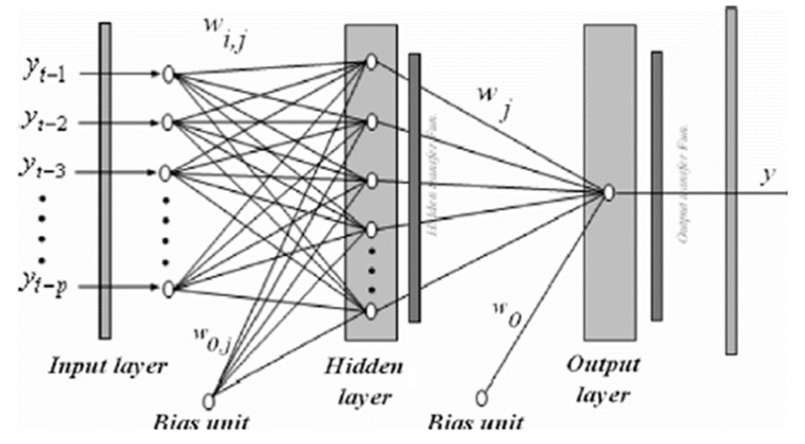
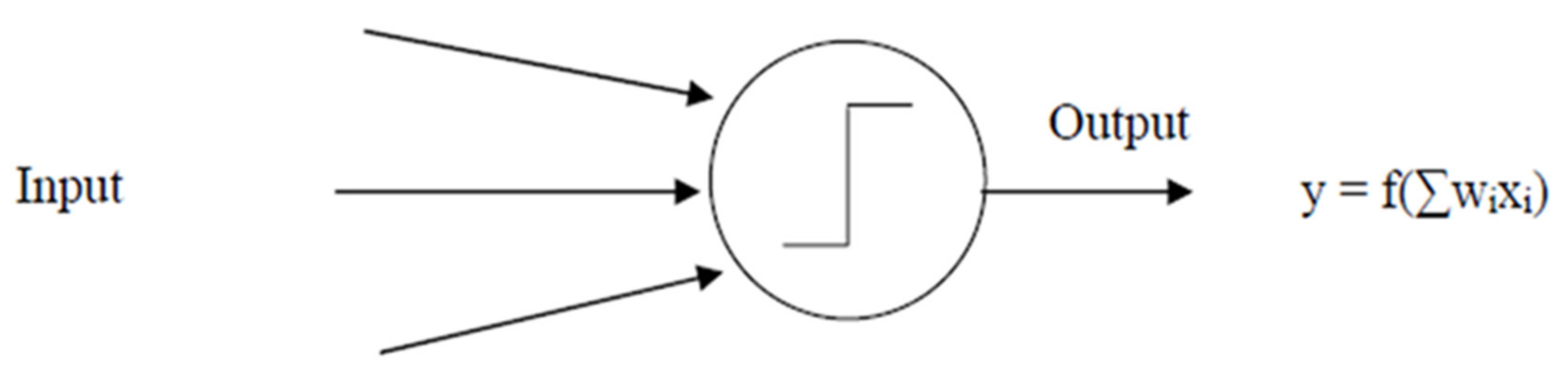
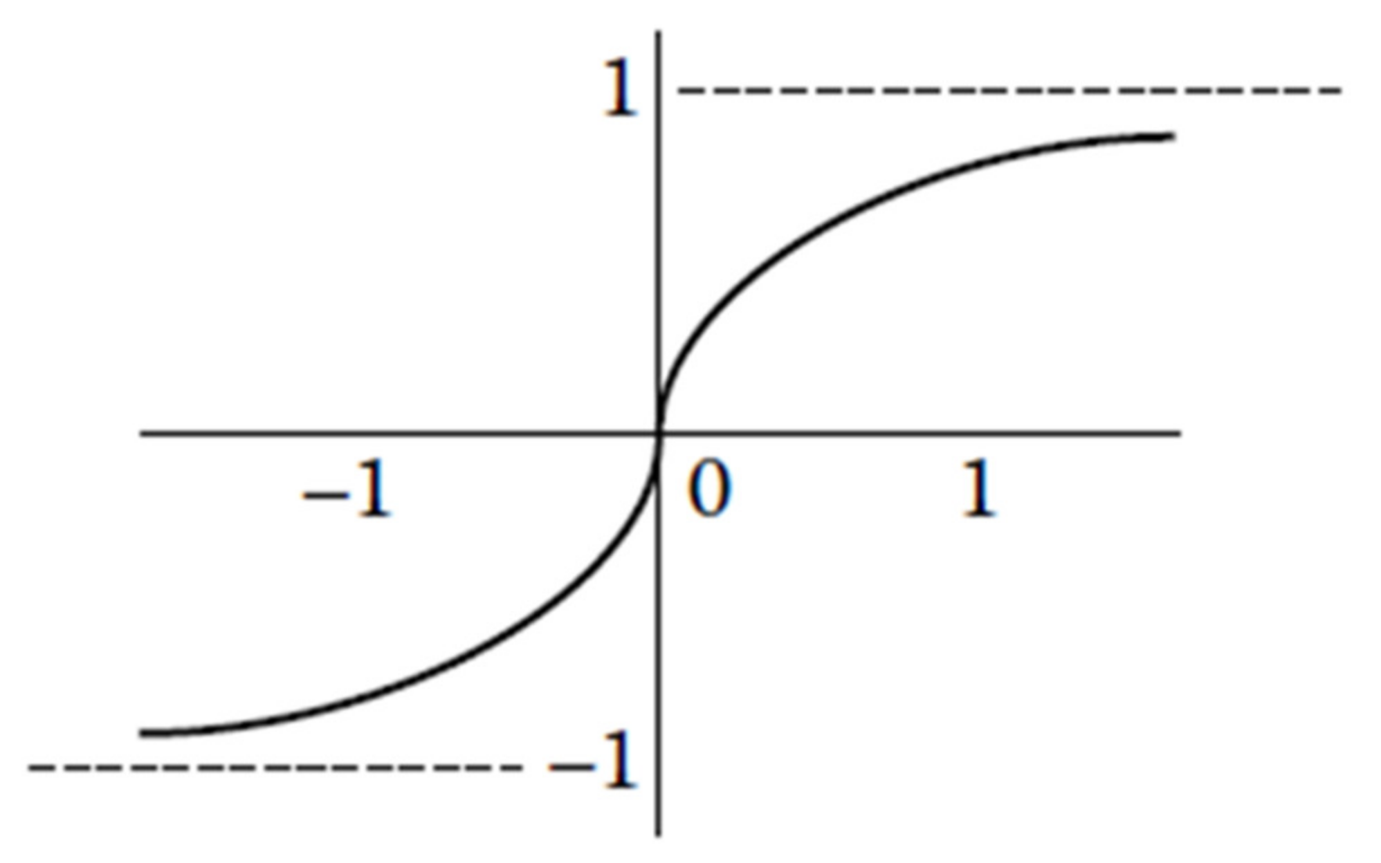
4.1.3. Artificial Neural Networks Model

Development of ANN model included preparing data as inputs and output, training, and testing the model. The data sets were randomly divided as follows: Training (85%), and Testing (15%). During training, the network was fed with inputs. The network then generated output. The network checked the results with correct answers and made corrections to internal connections while minimizing the errors. During testing inputs, they were paired with outputs which were provided. Testing is the same as training. Validation of the model was conducted after the model was developed. This process is referred to as running the model. Different data were used to run and check the application of the developed model. In model validation, only inputs were used to predict the sewer pipes condition.

4.1.4. Neural Networks Data Processing Software Selection

The data were stored in Microsoft Excel. It was processed and grouped into input and output variables. The created input data comprised of independent variables. These variables included pipe material, diameter, age, slope, depth, surface condition, soil type, corrosivity concrete, corrosivity steel, and pH. The created output data comprised the dependent variable. The dependent variable was sewer pipes condition rating.

The BrainMaker, a commercially available Simulator distributed by California Scientific Software, was used to develop the neural network model. BrainMaker used data stored in neural networks files. The neural network files were Definition (.def), Fact (.fct), and Testing (.tst).

Figure 5 shows the process of developing the neural network model. The steps that were used to develop the neural network model are as follows: (1) Acquire inspection and condition assessment data, (2) Prepare and process data. Categorical data were split into categories. The data were labeled into inputs and outputs, (3) Train network model. Twelve different neural network architectures were trained and obtained the optimal architecture with the lowest errors, (4) Tested network model. The architectures were tested using 15% of the data, (5) Run or validated model.

New data were used as a case study to validate the use of the model. Datasets were randomly divided: Training (70%), and Testing (30%) (IBM SPSS Neural network Software) and Training (85%), and Testing (15%) (Brain Maker Neural Network Software, California Scientific Software). The backpropagation algorithm was used in training the neural network model. Training involved presenting inputs to the network. The network uses the input variables to establish a relation between the inputs and outputs that are placed in NetMaker. The Netmaker tool is incorporated in BrainMaker. The data is processed in Netmaker and saved in the BrainMaker file.

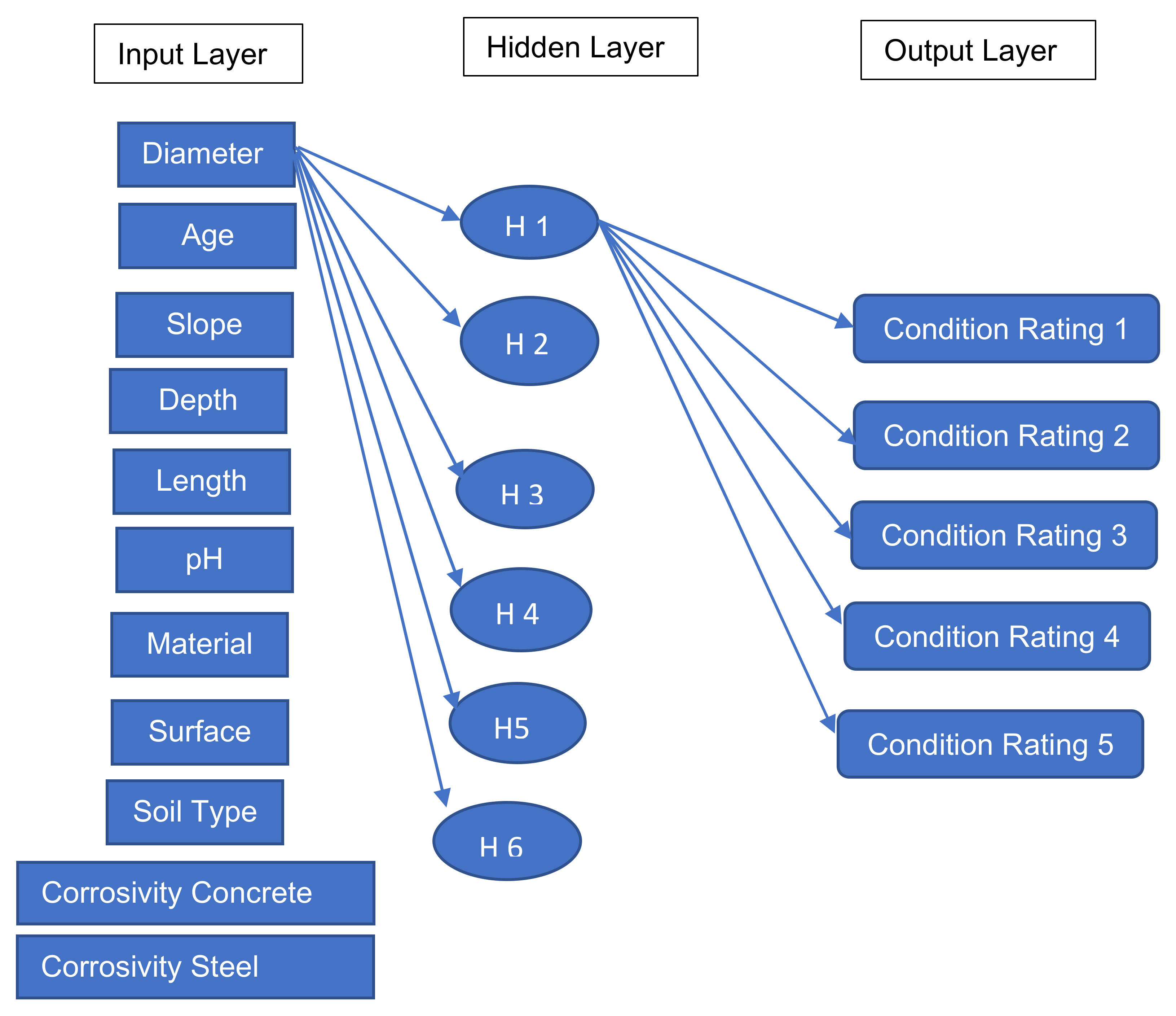
4.1.5. Neural Networks Architecture

The neural network architecture comprises three (3) layers, namely, input, hidden, and output layers. The hidden layer is known as hidden neurons. The number of neurons should be sufficient to provide optimal performance in the modeling prediction process. Too few or too many neurons will not enable the network to acquire knowledge that can be generalized for future predictions. There are three ways of determining the ideal number of hidden neurons. Equations (25) and (26) show two ways of calculating the number of hidden neurons.

$$\mathrm{Number} \mathrm{of} \mathrm{hidden} \mathrm{neurons}=\frac{\mathrm{of} \mathrm{Data} \mathrm{sets}-\mathrm{Outputs}}{\mathrm{C}\left(\#\mathrm{Input}+\#\mathrm{Output}+1\right)}$$

(25)

where, C = 2–5

$$\mathrm{Number} \mathrm{of} \mathrm{Neurons}=\left(\frac{\# \mathrm{Inputs}+\# \mathrm{Outputs}}{2}\right)$$

(26)

Equation (24) was suggested by BrainMaker Manual. In this study, Equation (24) was used to calculate the number of neurons.

= (22+1)/2 =12 Neurons.

In this study, starting at one neuron, the experiment was conducted from 1 neuron to 15 neurons. The neural network with the least testing error was selected (

Table 2. Training and Testing Errors.

Model #	Architecture	RMS Training	RMS Testing
1	22–4-1	0.3089	0.2745
2	22–5-1	0.3165	0.2857
3	22–6-1	0.2860	0.2620
4	22–7-1	0.3001	0.2647
5	22–8-1	0.3048	0.2720
6	22–9-1	0.3009	0.2662
7	22–10-1	0.3010	0.2751
8	22–11-1	0.3021	0.2716
9	22–12-1	0.3001	0.2730
10	22–13-1	0.3001	0.2695
11	22–14-1	0.3002	0.2712
12	22–15-1	0.3001	0.2700

).

Model #3 was found to be optimal with the least training and testing errors. Model #3 was chosen for model development.

4.2. Neural Networks Model Development

In BrainMaker, the network size of the optimal neurons was set at 6. Various training and testing tolerances were tested starting at 0.1 and 0.1, respectively. Training and testing tolerance of 0.3 and 0.3, respectively, was selected to be optimal, having the lowest training and testing errors. The training was achieved by the trial-and-error method, with weights randomly taking numbers in training the model. The training was stopped when the neural network reached the lowest training and testing errors. The training algorithm helps distribute the error to arrive at the minimum error. The information moves forward in the network to predict the output. While minimizing the error is achieved through several iterations, the backpropagation algorithm redistributes the error and adjusts the weights.

Figure 6 shows the ANN structure of the model. The structure was comprised of the input layer, hidden layer, and output layer. The input layer was comprised of independent variables. The input variables used were diameter, age, slope, depth, length, pH, material, surface condition, soil type, corrosivity concrete, and corrosivity steel. The hidden layer was comprised of the six neurons.

The output layer consisted of sewer pipe conditions 1, 2, 3, 4, and 5. Like it is shown for diameter parameter, there is a network of a relation between the input, hidden, and output layers. Similar relationships apply for all other parameters. This illustrates how ANN is working. This relationship in the network mirrors similar neural network illustrated by [30].

Table 3. Model Training and Testing Factors.

Total Factors	Good	Bad	Tolerance	Average Error	RMS Error
Training Configuration
2224	1599 (72%)	625 (28%)	0.3	0.2519	0.3048
Testing Configuration
392	334 (85%)	58 (15%)	0.3	0.227	0.2823

shows that the model learned 72% of the facts and predicted 85% of the testing factors.

5. Results and Discussion

In this section, results and discussions of multinomial logistic regression and neural networks models are presented. The accuracy of the models was discussed using a classification table, sensitivity, and specificity curves. ROC curve and model influence variables are also presented. The significance coefficients of the models are used to point out the variables that influence sewer pipe conditions. The confidence level used in the data analysis is 95%. The validation of multinomial logistic regression, including the justification of the results, is also discussed.

5.1. Performance of the Models

5.1.1. Multinomial Logistic Regression Model

The MLR correctly predicted 75% of the sewer pipe conditions overall. Prediction of sewer pipe condition 1 was 97% correct, with 3 percent incorrectly predicted. This demonstrated that the model had a high accuracy in predicting condition 1. According to the classification table conditions 2, 3, 4, and 5 were 0%, 28%, 4%, and 14% was correctly estimated. Sewer condition 1 datasets were 73% of the sewer pipe segments. Sewer pipes datasets condition 2, 3, 4, and 5 were 4%, 12%, 3%, and 7%, respectively, of the sewer pipes segments. This explains why the percent prediction correct rate was low in conditions 2, 3, 4, and 5 compared to condition 1. The prediction was consistent with the available datasets that were analyzed.

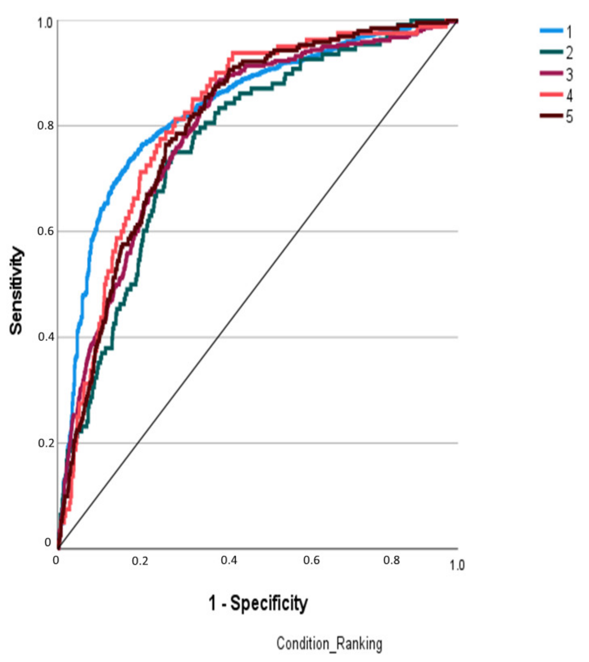
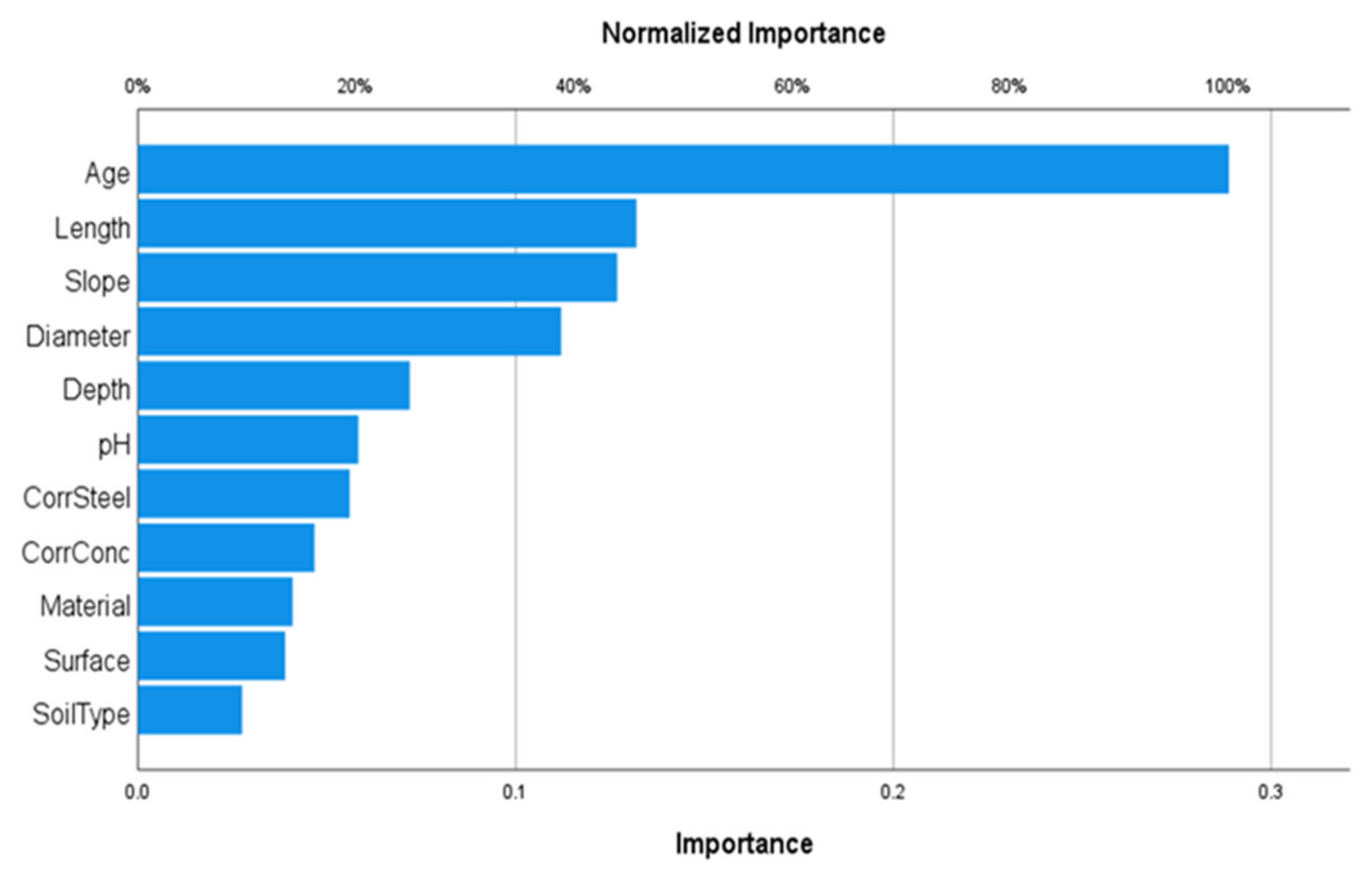
5.1.2. Neural Networks Model Performance

Figure 7 is derived from the metrics of measuring model performance as explained in the model development section. The area under the ROC curve provided in

Table 4. ROC Curve.

Condition	Area Under Curve
1	0.833
2	0.768
3	0.794
4	0.815
5	0.802

demonstrated the performance of the ANN model. When the area is close to one (1), it refers to the perfect model. When the area is greater than 0.7, it implies an acceptable model. According to Hosmer et al., 2013, when the area is close to one (1), it refers to the perfect model. When the area is greater than 0.7, it implies an acceptable model. Table 4 shows that the model is acceptable to be used in the prediction of sewer pipes conditions.

The accuracy of MLR and ANN model was compared. The ANN model was found to be better in predicting the sewer pipe condition compared to the MLR model. The prediction accuracy of the logistic regression model was 75% and that of the ANN model was 85%.

Ref. [34] defined sensitivity as True Positive Rate and specificity as True Negative Rate. These are metrics of measuring performance of a model.

5.2. Discussion

This study was set to develop logistic regression and neural networks sanitary sewer condition assessment prediction models. Observed datasets of independent and dependent variables were utilized to develop the models. The independent variables that influenced the condition ratings of the sewer pipes were presented in order of importance in Figure 6. Age, depth, slope, diameter, and depth, which are physical factors, were found to be the most important predictors compared to environmental factors. The significant variables that influence sewer pipes condition rating were diameter, age, length, pipe material (CONC), soil type (Loam), soil type (Clay), corrosivity concrete (Highway), and corrosivity concrete (Low). Influencing and non-influencing variables were determined by significance value (p < 0.05) based on a 95% Confidence Level.

Table 5. Significant Factors.

Factors	Sewer Pipe Condition
	1	2	3	4
Diameter	0.001	0.000	0.199	0.008
Age	0.000	0.001	0.000	0.807
Length	0.000	0.228	0.113	0.980
Material	0.503	0.025	0.001	0.280

shows factors that were found to be significant on the sewer pipe condition. Pipe diameter was found to be significant in sewer pipe conditions 1, 2, and 4 with a significant level of 95% the significant value p < 0.05. In condition 1, 2, and 4, the value p was 0.001, 0.000, and 0.008, respectively. Age was one of the significant variables. Age was found to be significant in sewer pipe conditions 1, 2, 3, and 4 with a significant value of p < 0.05. The significant p value in conditions 1, 2, and 3 were 0.000, 0.001, and 0.000, respectively. Pipe length was a significant factor in sewer pipe condition 1. The significant value of the pipe length was 0.000. Pipe material was a significant variable in the prediction model in sewer pipe conditions 2 and 3. The significant value of p was 0.025 and 0.001, respectively. The PVC material had most of the pipes that were in good condition.

Figure 8 shows significant factors. The significance of the of the factors is presented as a ratio and percentage (Normalized significance). Loam and clay soil types were found to be significant predictors. The significant value p was < 0.05 in condition 4. The significant values were 0.05 and 0.05, respectively. Corrosivity concrete (High) and corrosivity concrete (Low) variables are significant in the sewer pipes condition. The significant value p was <0.05 was found to be in condition 4. The significant values were 0.036 and 0.031, respectively. Depth, slope, corrosivity steel, and pH variables were found not to be significant in predicting sewer pipes condition.

5.3. Justification of Results

The model results were consistent with similar studies conducted by other authors. Ref. [3] found that age and material factors have a high impact on sewer pipe condition. In addition, Ref. [3] found that pipe diameter, depth, and slope were less significant in pipe condition. Significant p-Value and ODDs ratio (Exp(B)) generated in this study were compared with the results of other authors. In this research, the diameter was found to be significant in conditions 1, 2, and 4, with p values of 0.001, 0.000, and 0.008, respectively. The Exp(B) was 0.978, 0.923, and 0.951 for sewer pipes condition 1, 2, and 4, respectively. The Wald for sewer conditions 1, 2, and 4 were found to be 10.390, 12.975, and 7.020, respectively. The diameter of the pipe being significant was consistent with [12,18,35].

Age was another important factor that influences sewer pipes condition. In this study, age was found to be significant in predicting sewer pipe conditions. The p-value for age factor in conditions 1, 2, and 3 were 0.000, 0.001, and 0.000, respectively. Wald was 81.139, 11.57, and 15.222 for conditions 1, 2, and 3. The Exp(B) was 0.845, 0.968, and 0.974 for conditions 1 and 2, respectively. Refs. [12,13,18,35] found age to be a significant factor.

It was revealed that length was a significant factor in influencing the sewer pipes condition 1. The p-value was 0.000, and Wald and Exp (0.999) were 20.852 and 0.999, respectively. This was confirmed by a study conducted by [12,18,35]. Pipe material (Conc) was a significant factor in influencing sewer pipe conditions. In conditions 2, p-value, Wald, and Exp(B) were 0.025, 5.030, and 0.472, respectively. In condition 3, p-value, Wald, and Exp(B) were 0.001, 10.828, and 2.089, respectively. Pipe material was found to be insignificant in conditions 1 and 4. This is consistent with [12].

Soil type (Clay), soil type (Loam), and soil type rock were revealed to be significant in sewer conditions 2, 3, and 4. In condition 2 for clay soil p-value, Wald, and Exp(B) were 0.05, 3.89, and 9.12, respectively. In condition 3 for clay soil, p-value, Wald, and Exp(B) were 0.021, 0.021, and 1.153, respectively. Similarly, for loam soil, the p-value, Wald, and Exp(B) were 0.05, 3.89, and 9.12, and for loam soil, the p-value, Wald, Exp(B) for soil type (Rock) was 0.018, 0.0.18, and 0.864. Ref. [18] found that soil type is a significant variable in the prediction of sewer pipe condition. In condition 4, soil type clay and loam have Wald of 3.89 and 3.93, p-value 0.05 and 0.05, and Exp(B) of 9.12 and 9.68, respectively.

Corrosivity concrete was found to be significant in influencing pipe conditions. The p-value, Wald, and Exp(B) were 0.036, 4.411, and 0.096, respectively. Ref. [18] found corrosivity to be of very high significance. The model prediction accuracy in this research was compared with other authors.

Table 6. Prediction Accuracy.

Model	Author	Prediction Accuracy	Dissertation Results	Deviation
Multinomial Logistic Regression	[30]	52%	75%	23%
	[1]	65%		10%
	[18]	62%		13%
	[37]	65%		10%
	[27]	72%		3%
	[13]	55–90.9%		15.9–20%
Artificial Neural Network	[36]	72–82%	85%	3–13%
	[28]	84%		1%
	[13]	70–93.6%		8.6–15%

shows that different authors obtained varying prediction accuracy. Collected data could be a factor in varying prediction accuracy. Ref. [36] stated that the usefulness of a model will be increased with more data.

Comparison of MLR and ANN Models and Conclusions

It can be concluded that MLR and ANN models were developed to predict sanitary sewer pipe conditions. The models were developed, validated, and tested in prediction sewer pipe condition scores to prioritize pipes to be rehabilitated and/or replaced and further condition assessment. The developed models added knowledge in the tools used to predict sanitary sewer pipes condition. Predicting and knowing the sanitary sewer pipes condition rating score would be beneficial to policymakers, and sanitary sewer utilities managers in prioritizing rehabilitation and/or replacement of sanitary sewer pipes.

The logistic model was built with 80% of the randomly selected dataset. The randomly remaining 20% of the data were utilized in the validation of the model. The ANN model was trained, validated, and tested. The feed-forward network with a backpropagation learning algorithm was employed. Based on the logistic model results, the significant physical factors influencing sanitary pipes failure included diameter, age, pipe material, and length. Soil type was the environmental factor that influenced sanitary sewer pipes failure.

The accuracy of the performance of the MLR and ANN was found to be 75% and 85%, respectively. Concerning the main objective of this research, it was determined that the use of ANN model provided more accurate prediction of sanitary sewer pipes condition by testing the results of the condition rating values.

The importance of the independent variables was found to be in the following order. Age (100%), Diameter (80%), Slope (62%), Length (62%), Flow (60%), pH (40%), Corrosivity Steel (38%), Soil Type (36%), Depth (35%), Pipe Material (25%), Surface Condition (22%), and Corrosivity (20%). Diameter (p value = 0.001 < 0.05), age (p value = 0.000 < 0.05), length (p value = 0.000 < 0.05), pipe material (CONC) (p value = 0.001 < 0.05)), soil type (Loam) (p value = 0.05 < 0.05), soil type (Clay) (p value = 0.001 < 0.05), corrosivity concrete (p value = 0.001 < 0.05), and corrosivity concrete (Low) (p value = 0.001 < 0.05).

6. Recommendations for Future Research

This study raised several important points to be considered for future research. The data for this dissertation was collected from the Dallas Water Utilities. Other cities should be included in future studies and results compared with results of this research. There is a need for utilizing more datasets to increase the accuracy of the prediction models. Data collected for analysis should include more uniformly distributed number of observations in every condition. More training and testing of the ANN model are needed to fine tune and validate its prediction strength for conditions 4 and 5. Excluded pipe material types could be included for further model development. These models can be improved by utilizing wastewater type and volumetric flow rate variables in their prediction and comparison.

References

1. Mohammadi, M.M.; Najafi, M.; Kaushal, V.; Serajiantehrani, R.; Salehabadi, N.; Ashoori, T. Sewer Pipes Condition Prediction Models: A State-of-the-Art Review. Infrastructures 2019, 4, 64. [Google Scholar] [CrossRef] [Green Version]
2. Kaushal, V.; Najafi, M.; Serajiantehrani, R. Environmental Impacts of Conventional Open-Cut Pipeline Installation and Trenchless Technology Methods: State-of-the-Art Review. J. Pipeline Syst. Eng. Pr. 2020, 11, 03120001. [Google Scholar] [CrossRef]
3. Hawari, A.; Alkadour, F.; Elmasry, M.; Zayed, T. A state of the art review on condition assessment models developed for sewer pipelines. Eng. Appl. Artif. Intell. 2020, 93, 103721. [Google Scholar] [CrossRef]
4. American Society of Civil Engineers (ASCE). 2021 Report Card for America’s Infrastructure; ASCE: Washington, DC, USA, 2017. [Google Scholar]
5. Serajiantehrani, R.; Najafi, M.; Mohammadi, M.M.; Kaushal, V. Framework for Life-Cycle Cost Analysis of Trenchless Renewal Methods for Large Diameter Culverts. In Pipelines 2020; American Society of Civil Engineers: Reston, VI, USA, 2020; pp. 309–320. [Google Scholar]
6. Wirahadikusumah, R.; Abraham, D.M.; Castello, J. Markov decision process for sewer rehabilitation. Eng. Constr. Arch. Manag. 1999, 6, 358–370. [Google Scholar] [CrossRef]
7. Alegre, H. Is strategic asset management applicable to small and medium utilities? Water Sci. Technol. 2010, 62, 2051–2058. [Google Scholar] [CrossRef] [PubMed]
8. Bruaset, S.; Rygg, H.; Sægrov, S. Reviewing the Long-Term Sustainability of Urban Water System Rehabilitation Strategies with an Alternative Approach. Sustainability 2018, 10, 1987. [Google Scholar] [CrossRef] [Green Version]
9. Najafi, M. Pipeline Infrastructure Renewal and Asset Management; Mc-Graw-Hill Education: New York, NY, USA, 2016. [Google Scholar]
10. Khan, Z.; Zayed, T.; Moselhi, O. Structural Condition Assessment of Sewer Pipelines. J. Perform. Constr. Facil. 2010, 24, 170–179. [Google Scholar] [CrossRef]
11. Malek Mohammadi, M.; Najafi, M.; Kermanshachi, S.; Kaushal, V.; Serajiantehrani, R. Factors Influencing the Condition of Sewer Pipes: State-of-the-Art Review. J. Pipeline Syst. Eng. Pract. 2020, 11, 03120002. [Google Scholar] [CrossRef]
12. Lubini, A.T.; Fuamba, M. Modeling of the deterioration timeline of sewer systems. Can. J. Civ. Eng. 2011, 38, 1381–1390. [Google Scholar]
13. Khudair, H.B.; Khalid, K.G.; Jbbar, K.R. Condition Prediction Model of Deteriorated Trunk Sewer using Mul-tinomial Logistic Regression and Artificial Neural Network. Int. J. Civ. Eng. Technol. 2019, 10, 93–104. [Google Scholar]
14. Muhlbauer, K. Pipeline Risk Management Manual Ideas, Techniques, and Resources, 3rd ed.; Elsevier: Oxford, UK, 2004. [Google Scholar]
15. Hou, P.; Yi, X.; Dong, H. A Spatial Statistic Based Risk Assessment Approach to Prioritize the Pipeline Inspection of the Pipeline Network. Energies 2020, 13, 685. [Google Scholar] [CrossRef] [Green Version]
16. Caradot, N.; Riechel, M.; Fesneau, M.; Hernandez, N.; Torres, A.; Sonnenberg, H.; Eckert, E.; Lengemann, N.; Waschnewski, J.; Rouault, P. Practical benchmarking of statistical and machine learning models for predicting the condition of sewer pipes in Berlin, Germany. J. Hydroinformatics 2018, 20, 1131–1147. [Google Scholar] [CrossRef] [Green Version]
17. Syachrani, S.; Jeong, H.D.; Chung, C.S. Advanced criticality assessment method for sewer pipeline assets. Water Sci. Technol. 2013, 67, 1302–1309. [Google Scholar] [CrossRef]
18. Laakso, T.; Kokkonen, T.; Mellin, I.; Vahala, R. Sewer Condition Prediction and Analysis of Explanatory Factors. Water 2018, 10, 1239. [Google Scholar] [CrossRef] [Green Version]
19. Najafi, M.; Gokhale, S. Trenchless Technology Pipeline and Utility Design, Construction, and Renewal; McGraw-Hill: New York, NY, USA, 2005. [Google Scholar]
20. Burn, S.; Marlow, D.; Tran, D. Modelling asset lifetimes and their role in asset management. J. Water Supply Res. Technol. 2010, 59, 362–377. [Google Scholar] [CrossRef]
21. Hosmer, D.W., Jr.; Lemeshow, S.; Sturdivant, R.X. Applied Logistic Regression; John Wiley & Sons. Inc.: Columbus, OH, USA, 2013. [Google Scholar]
22. Khashei, M.; Bijari, M. An artificial neural network (p,d,q) model for timeseries forecasting. Expert Syst. Appl. 2010, 37, 479–489. [Google Scholar] [CrossRef]
23. Elmasry, M.; Hawari, A.; Zayed, T. Defect based deterioration model for sewer pipelines using Bayesian belief networks. Can. J. Civ. Eng. 2017, 44, 675–690. [Google Scholar] [CrossRef]
24. Ward, B.; Savić, D.A. A multi-objective optimization model for sewer rehabilitation considering critical risk of failure. Water Sci. Technol. 2012, 66, 2410–2417. [Google Scholar] [CrossRef] [Green Version]
25. Peponi, A.; Morgado, P.; Trindade, J. Combining Artificial Neural Networks and GIS Fundamentals for Coastal Erosion Prediction Modeling. Sustainability 2019, 11, 975. [Google Scholar] [CrossRef] [Green Version]
26. Rokstad, M.M.; Ugarelli, R.M. Evaluating the role of deterioration models for condition assessment of sewers. J. Hydroinformatics 2015, 17, 789–804. [Google Scholar] [CrossRef] [Green Version]
27. Chughtai, F.M.; Zayed, T. Infrastructure Condition Prediction Models for Sustainable Sewer Pipelines. J. Perform. Constr. Facil. 2008, 5, 333–341. [Google Scholar] [CrossRef]
28. Kulandaivel, G. Sewer Pipeline Condition Prediction Using Neural Network Models. Master’s Thesis, Michigan State University, East Lansing, MI, USA, 2004. [Google Scholar]
29. Adamowski, J.; Fung Chan, H.; Prasher, S.O.; Ozga-Zielinski, B.; Sliusarieva, A. Comparison of multiple linear and nonlinear regression, autoregressive integrated moving average, artificial neural network, and wavelet artificial neural network methods for urban water demand forecasting in Montreal, Canada. Water Resour. Res. 2012, 48, W01528. [Google Scholar] [CrossRef]
30. Chakraverty, S.; Mall, S. Artificial Neural Networks for Engineers and Scientists: Solving Ordinary Differential Equations; CRC Press: Boca Raton, FL, USA, 2017. [Google Scholar]
31. Salman, B. Infrastructure Management and Deterioration Risk Assessment of Wastewater Collection Systems. Ph.D. Thesis, University of Cincinnati, Cincinnati, OH, USA, 2010. [Google Scholar]
32. Syachrani, S. Advanced Sewer Asset Management Using Dynamic Deterioration Models. Ph.D. Thesis, Oklahoma State University, Stillwater, OK, USA, 2010. [Google Scholar]
33. Vahidi, E.; Jin, E.; Das, M.; Singh, M.; Zhao, F. Environmental life cycle analysis of pipe materials for sewer systems. Sustain. Cities Soc. 2016, 27, 167–174. [Google Scholar] [CrossRef]
34. Yin, X.; Chen, Y.; Bouferguene, A.; Al-Hussein, M.; Russell, R.; Kurach, L. A neural network-based approach to predict the condition for sewer pipes. In Proceedings of the Construction Research Congress 2020: Infrastructure Systems and Sustainability—Selected Papers from the Construction Research Congress 2020, Tempe, AZ, USA, 8–10 March 2020. [Google Scholar] [CrossRef]
35. Tscheikner-Gratl, F.; Mikovits, C.; Rauch, W.; Kleidorfer, M. Adaptation of sewer networks using integrated rehabilitation management. Water Sci. Technol. 2014, 70, 1847–1856. [Google Scholar] [CrossRef] [PubMed]
36. Geem, Z.W.; Tseng, C.-L.; Kim, J.; Bae, C. Trenchless Water Pipe Condition Assessment Using Artificial Neural Network. In Pipelines 2007; American Society of Civil Engineers: Reston, VI, USA, 2007; pp. 1–9. [Google Scholar]
37. Sousa, V.; Matos, J.P.; Almeida, N.; Matos, J.S. Risk assessment of sewer condition using artificial intelligence tools: Application to the SANEST sewer system. Water Sci. Technol. 2014, 69, 622–627. [Google Scholar] [CrossRef] [PubMed]
Figure 1. Neural Network Structure [27].
Sustainability 14 05549 g001
Figure 2. Schematic Diagram of a Single Artificial Neuron [28,29].
Sustainability 14 05549 g002
Figure 3. Plot on Bipolar Sigmoid Function.
Sustainability 14 05549 g003
Figure 4. Study Methodology.
Sustainability 14 05549 g004
Figure 5. ANN Model Development Procedure [28].
Sustainability 14 05549 g005
Figure 6. ANN Structure.
Sustainability 14 05549 g006
Figure 7. Plot of Model Sensitivity and Specificity.
Sustainability 14 05549 g007
Figure 8. Influence of Variables.
Sustainability 14 05549 g008