Vision Robot Path Control Based on Artificial Intelligence Image Classification and Sustainable Ultrasonic Signal Transformation Technology

Abstract

The unsupervised algorithm of artificial intelligence (AI), named ART (Adaptive Resonance Theory), is used to first roughly classify an image, that is, after the image is processed by the edge filtering technology, the image window is divided into 25 square areas of 5 rows and 5 columns, and then, according to the location of the edge of the image, it determines whether the robot should go straight (represented by S), turn around (represented by A), stop (T), turn left (represented by L), or turn right (represented by R). Then, after sustainable ultrasonic signal acquisition and transformation into digital signals are completed, the sustainable supervised neural network named SGAFNN (Supervised Gaussian adaptive fuzzy neural network) will perform an optimal path control that can accurately control the traveling speed and turning of the robot to avoid hitting walls or obstacles. Based on the above, this paper proposes the use of the ART operation after image processing to judge the rough direction, followed by the use of the ultrasonic signal to carry out the sustainable development of artificial intelligence and to carry out accurate speed and direction SGAFNN control to avoid obstacles. After simulation and practical evaluations, the proposed method is proved to be feasible and to exhibit good performance.

1. Introduction

ART (Adaptive Resonance Theory) is an unsupervised neural network developed in the 1980s. The main principle is to compare the output vector of the existing category by calculating the matching value according to the input vector. If it passes the test of similar value, it belongs to this type of output vector; otherwise, continue to compare until all the comparisons are completed; if they do not match, a new type of output vector will be generated [1,2,3]. The advantage of this method is that the threshold of matching value and similarity value can be adjusted to maintain the stability and plasticity of the classification. When the stability is high, there are fewer categories to be classified, and when the plasticity is improved, there are more categories. Therefore, how high the matching value should be set will affect the stability and plasticity of the judgment. These two values are mutually exclusive, and the best matching value is usually obtained by trial-and- error [4,5,6,7].

Regarding the deep learning technology of artificial intelligence of image recognition, the convolution neural network (CNN) was first introduced in recent years, and the sustainable research of robots combined with various control methods has also made breakthroughs. A sustainable architecture is proposed to control the robot after image processing, and the method is to use multi-layer deep feature fusion technology and fusion to perform accurate image classification. Usually, a camera is used to capture images and to conduct subsequent sustainable artificial intelligence control [8,9]. Position recognition of the robot has also been developed, such as farm management, robotic path planning, arable land detection from photos captured by drones with cameras, and the development of sustainable applications as more advanced features in agriculture. These applications are developed by many different methods, such as particle swarm optimization (PSO), fuzzy-PDC, image processing and neural networks, etc., to allow the robot controller to achieve optimal path control [10,11,12,13,14].

In general, the Gaussian membership function of fuzzy logic has only one variable, which controls the type of the Gaussian function. In the 1990s, some researchers proposed a new Gaussian function with four variables: three for the antecedent part and the other for the consequent part [15]. Therefore, these four variables can be adjusted by neural network mathematical derivation operations to achieve the effect of supervised learning. Then, combined with sliding control, more precise control performances can be obtained [16]. The image control mentioned in the previous paragraph is only used to obtain initial rough control. In order to obtain better control performance, there must be a design concept of sustainability. This paper proposes a method, which is to use an ultrasonic signal to assist the robot controller to obtain better performance. After all, if the robot is completely controlled by images, the computing burden of the hardware GPU (Graphic processing unit) will be very large, so the design concept here is that the front-end rough images are classified as go straight (represented by S), turn around (represented by A), stop (T), turn left (represented by L), or turn right (represented by R), which will be obtained as one of five results. Then, there is the sustainability control, which is controlled by a supervised Gaussian adaptive fuzzy neural network (SGAFNN); this input is the ultrasonic signal. The advantage of this design is to reduce the computational burden of the system and avoid the burst operation of SGAFNN. In this paper, a SGAFNN design was developed for mobile robots. A standalone camera is used as an image sensor to obtain image data, and the surrounding ultrasonic sensors are used to complement the main sensor to obtain all necessary data, then to generate the required path according to the control algorithm SGAFNN, and finally to follow this control law to achieve the purpose of avoiding collisions with walls and obstacles.

Fuzzy neural network (FNN) technologies have been developed successfully. Many different types of FNNs have been proposed in every area of research. FNN has the potential learning ability to cope with very complex dynamic actions. This allows a neural network to push reasonable input output maps such as to approximate any function with the required hidden layers of a neural network. It also allows a designed controller that does not depend on exact mathematical models [17,18]. In general, the layers of membership functions and output layers should be adaptive [19,20]. A Gaussian membership function, also known as a radial basis function (RBF), can be applied to approximate any continuous function and smooth function [21,22]. Adaptive FNN (AFNN) is also a strong tool, because its many parameters can be tuned online such that the learning speed and robustness can be guaranteed. Meanwhile, this is mainly combined with the traditional PID control theory, adding adjusted parameters to eliminate disturbance and uncertainties, so that the final steady-state error can converge to zero [22,23]. The most useful method is the projection theorem [24] because it has easy implementation, a confident learning ability, and reliable stability.

The motivation of the research is to divide the control steps into two parts. If the first part can be solved, the calculation of the second part will not be required. For example, in a spacious passage, the problem can be solved by using images processing and ART. However, if it reaches a narrow passage, it is necessary to carry out sustainable development of AI and carry out more precise path control. In this paper, a sustainable artificial intelligence and digital signal transformation module design concept is proposed. That is, in first is a simple design that then has an end complex design. The front-end only judges five possibilities. If it is S, then the back-end SGAFNN controls the speed. If it is R or L, then the back-end SGAFNN controls the angle and decelerates velocity. If it is A or T, it does not need to go through SGAFNN. Through such a sustainable artificial intelligence design concept, it can be expanded in the future, that is, according to system requirements, design modules can be superimposed, which we call sustainable artificial intelligence (SAI). In general, the best way to compensate for design errors or obtain system stability is to add a sliding controller (SC) [25,26,27,28]. Because this GAFNN is just a neural network controller, in order to ensure stability and accuracy, the best method is to combine it with an SC to become a full controller. Because the GAFNN controller is mainly looking for the direction of the control stable point, an SC has the ability to make the system stay at the absolute stable point of the system and resist disturbance and system uncertainty. The proposed method is to give the gain of control on-the-fly to let the error of the optimized GAFNN controller and the full controller approach zero. When we complete the design of the SGAFNN controller, the hardware can obtain reliable and applicable fuzzy if-then memory vector parameters. Based on these parameters, it can be actually written into the hardware program memory to become Fuzzy Associative Memory (FAM). As for the SC, it is the instant control rate to compensate for the change of the uncertainty limit. Finally, the performance comparison of the proposed SGAFNN for robotics shows that the performance and stability are guaranteed. The simulation results also show that better performance, robustness and stability are gained. In the practical implementation of robotics, the performance of the proposed method is shown to be effective, reliable, and excellent.

2. Sustainable Artificial Intelligence (SAI) Controller Design

This section is mainly divided into three subsections to discuss how to determine the direction from the initial ART image classification, and then sustainably use the ultrasonic signal to control the robot more accurately to avoid encountering obstacles. This relies on the artificial intelligence technology of neural networks and sliding mode control, which are described as follows.

2.1. ART Controller Design

First all, the algorithm of ART is briefly described in

Table 1. The algorithm of ART.

Step 1	Set the initial network weightings.
Step 2	Enter the vector values of the training data.
Step 3	Calculate the match values for all categories of existing classifications.
Step 4	Find the one with the largest matching value and calculate its similarity value with this category.
Step 5	If it exceeds the similarity value, it belongs to this category, otherwise, it is a new generated category.
Step 6	Return to step 2, repeat the calculation of all input data until they are finished and stop the calculation of the program.

below:

After all, ART can only make five preliminary possible direction judgments (i.e., go straight (S), left turn (L), right turn (R), around turn (A), stop (T)) based on image processing; it cannot achieve precise control, so it is necessary to use the ultrasonic distance sensing signal to achieve a follow-up sustainable accurate control.

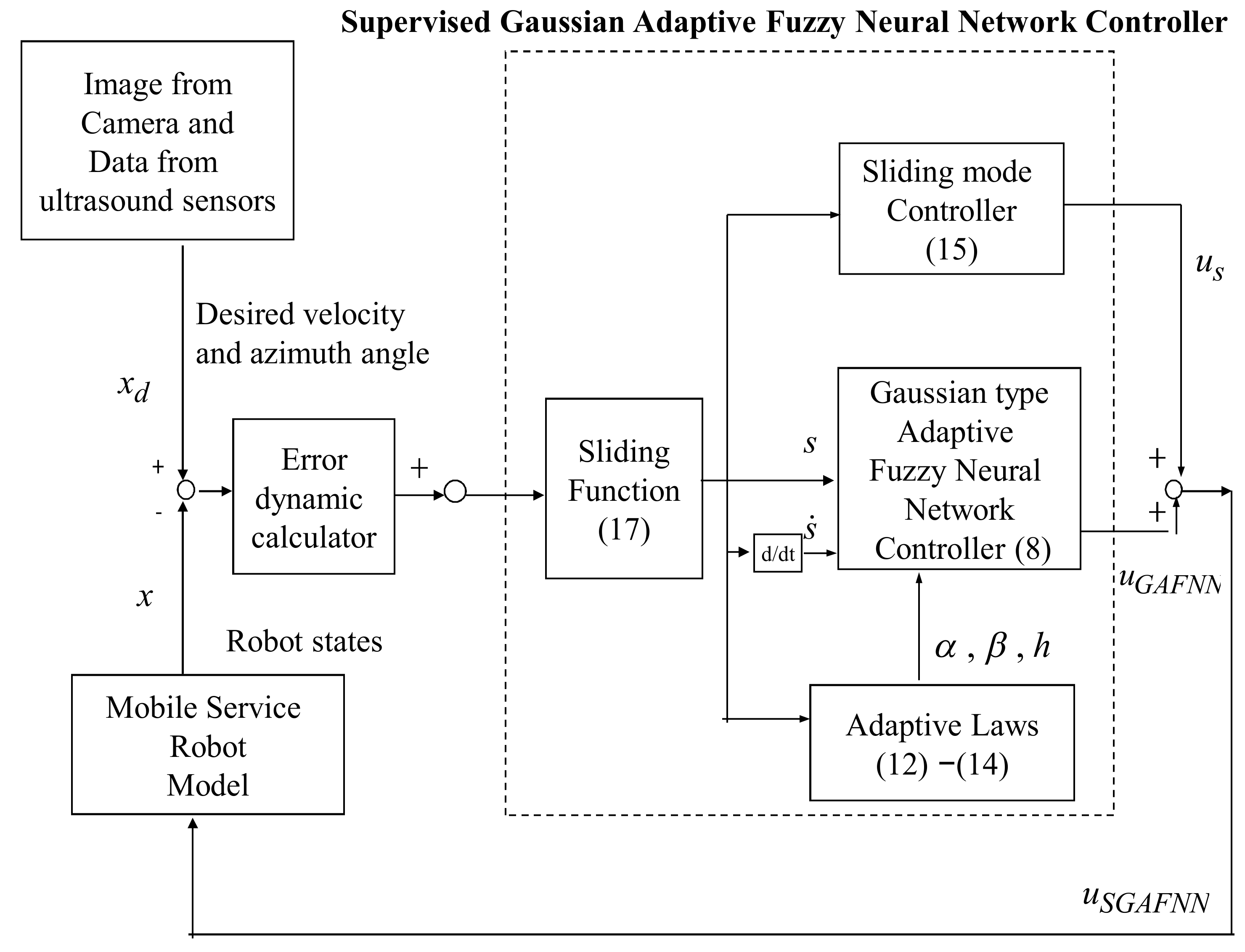
2.2. Supervised Gaussian Adaptive Fuzzy Neural Network (SGAFNN) Controller Design

When the image of the first stage is classified as S, L, or R, the system will automatically enter the SGAFNN control of the second stage. This section mainly discusses the derivation of this theory. Regarding this, a nonlinear system’s mathematical model is as below:

$$\dot{\mathit{x}}(\mathit{t})=\mathit{F}+\mathit{G}\mathit{u}+\mathit{d}$$

(1)

where $\mathit{x}(\mathit{t})$ and $\mathit{u}(\mathit{t})$ are n dimensional state vectors that represent state and control input vectors $\mathit{d}(\mathit{t})$ is unknown n dimensional disturbance and uncertainties with a known upper bound $‖\mathit{d}(\mathit{t})‖\le \mathit{D}$, which is a norm. Because $\mathit{F}$ and $\mathit{G}$ depend on $\mathit{x}(\mathit{t})$, so in the following parts, for simplicity, the symbols of $\mathit{F}$, $\mathit{G}$, $\mathit{x}$, $\mathit{u}$, and $\mathit{d}$ are used instead.

Suppose an optimize controller ${\mathit{u}}^{*}$ exists in order to overcome unknown system parameters; this is not easily achieved. A sliding Gaussian adaptive fuzzy neural network (SGAFNN) controller is proposed to approximate this optimized controller. Meanwhile, a sliding controller is designed to compensate for those uncertainties and disturbances and for the approaching error between the SGAFNN and the optimize controller. According to the universal approximation theorem, optimal ${\mathit{u}}^{*}$ should exist. In the following derivation, for the sake of simplicity, the state vector and control vector are discussed separately as every single state and control input which is denoted as $\mathit{x}$ and $\mathit{u}$. The reasonable error bound can be assumed during the design period. Then, a reasonable system stability bound can be guaranteed.

For a Gaussian adaptive fuzzy neural network (GAFNN) system, the simplified expression can be expressed as

$$\begin{array}{l}{\mathit{R}}_{\mathit{i}}:\mathit{I}\mathit{f} {\mathit{y}}_1={\mathit{z}}_{\mathit{i}1} \mathit{a}\mathit{n}\mathit{d}\dots {\mathit{y}}_{\mathit{n}}={\mathit{z}}_{\mathit{i}\mathit{n}}\\ \begin{array}{cc}& \mathit{T}\mathit{h}\mathit{e}\mathit{n} \end{array}{\mathit{u}}_{\mathit{i}1}={\mathit{P}}_{\mathit{i}1}{}_{}^{} \mathit{a}\mathit{n}\mathit{d}\dots {\mathit{u}}_{\mathit{i}\mathit{p}}={\mathit{P}}_{\mathit{i}\mathit{p}}\end{array}$$

(2)

where ${\mathit{R}}_{\mathit{i}}$ denotes the ith fuzzy rule; ${\mathit{z}}_{\mathit{i}\mathit{k}}$ is the fuzzy set in the antecedent associated with the kth input variable at the ith fuzzy rule; and ${\mathit{P}}_{\mathit{i}\mathit{j}}$ denotes a constant associated with the jth output variable in consequence of the ith fuzzy rule.

The inferred output is

$${\mathit{u}}_{\mathit{j}}^{\ast }={\frac{{\displaystyle \sum _{\mathit{i}=1}^{\mathit{r}}{\mathit{h}}_{\mathit{i}}}{\mathit{P}}_{\mathit{ij}}}{{\displaystyle \sum _{\mathit{i}=1}^{\mathit{r}}{\mathit{h}}_{\mathit{i}}}}}_{}^{},\mathit{j}=1,\dots ,\mathit{p};$$

(3)

where ${\mathit{h}}_{\mathit{i}}={\mathit{u}}_{{\mathit{A}}_{\mathit{i}1}}{(\mathit{x}}_1)\cdot {\mathit{u}}_{{\mathit{A}}_{\mathit{i}2}}{(\mathit{x}}_2)\dots {\mathit{u}}_{{\mathit{A}}_{\mathit{in}}}{(\mathit{x}}_{\mathit{n}})$ is the inferred grade of the ith fuzzy rule and ${\mathit{u}}_{{\mathit{A}}_{\mathit{ik}}}{(\mathit{x}}_{\mathit{k}})$ is the membership function grade of fuzzy variable.

The commonly used Gaussian-type membership function is defined as [15,16]

$${\mathit{f}}_{\mathit{ij}}{(\mathit{x}}_{\mathit{i}})={\mathit{e}}^{-{{\left[\right(\mathit{x}}_{\mathit{i}}-{\alpha }_{\mathit{ij}}{)/\beta }_{\mathit{ij}}]}^2};$$

(4)

where ${\mathit{f}}_{\mathit{i}\mathit{j}}({\mathit{x}}_{\mathit{i}})$ is the j-th membership function of the Gaussian membership function. The neural network is constructed as in Figure 1.

The (A) to (D) of left part stand for the antecedent parts of fuzzy rules, and the (E) to (F) of right part stand for the consequent parts of fuzzy rules. For every rule grade ${\mathit{h}}_{\mathit{i}}$ is calculated to get the result of Equation (3). The meanings of ${\alpha }_{\mathit{ij}}$ and ${\beta }_{\mathit{ij}}$ and ${\mathit{h}}_{\mathit{i}}$ are the antecedent and consequent parts of fuzzy rules which is equivalent to ${\mathit{W}}_{\mathit{i}\mathit{j}}$ of Equation (3).

The neural network weightings calculations are got from the back-propagation algorithm. The calculation equations of every layers of neural networks are got as following descriptions.

$${{\displaystyle \mathsf{\delta }}}_{\mathit{j}}^{\mathit{M}}={\mathit{f}}^{\prime }({{\displaystyle \mathit{i}}}_{\mathit{j}}^{\mathit{M}}){\displaystyle \sum _{\mathit{i}=1}^{\mathit{m}}{(\mathit{y}}_{\mathit{di}}-{\mathit{y}}_{\mathit{i}})\frac{\partial {\mathit{y}}_{\mathit{i}}}{\partial {\mathsf{\mu }}_{\mathit{j}}}}$$

(5)

where $\mathit{f}(\cdot )$ is the function of Equation (5), ${\mathsf{\delta }}_{\mathit{j}}^{\mathit{M}}$ is the delta quantities in the jth unit at the output layer M; ${\mathit{i}}_{\mathit{j}}^{\mathit{M}}$ is the input to the jth unit at the output layer M; ${\mathit{y}}_{\mathit{d}\mathit{i}}$ is the ith desired system output; ${\mathit{y}}_{\mathit{i}}$ is the ith system output; ${\mathsf{\mu }}_{\mathit{j}}$ is the output through the jth unit at the output layer M, and $\frac{\partial {\mathit{y}}_{\mathit{i}}}{\partial {\mathit{u}}_{\mathit{j}}}$ is the partial derivative value of ${\mathit{y}}_{\mathit{i}}$ with respect to ${\mathsf{\mu }}_{\mathit{j}}$.

For hidden layer of (E):

$${\mathsf{\delta }}_{\mathit{j}}^{\mathit{k}}={\mathit{f}}^{\prime }({\mathit{i}}_{\mathit{j}}^{\mathit{k}}){\displaystyle \sum _{\mathit{l}}{\mathsf{\delta }}_{\mathit{l}}^{\mathit{k}+1}{\mathit{w}}_{\mathit{j}\mathit{l}}^{\mathit{k},\mathit{k}+1}}({\displaystyle \prod _{\mathit{i}\ne \mathit{j}}^{}{\mathit{w}}_{\mathit{i}\mathit{j}}^{\mathit{k},\mathit{k}+1}{\mathit{o}}_{\mathit{i}}^{\mathit{k}})}$$

(6)

where all variables can be easy understood by the previous descriptions.

Then, the calculation of weighting equations can be got as follows:

$${\mathit{w}}_{\mathit{ij}}^{\mathit{k}-1,\mathit{k}}(\mathit{t}+1)={\mathit{w}}_{\mathit{ij}}^{\mathit{k}-1,\mathit{k}}\left(\mathit{t}\right)+{\mathsf{\eta }\mathsf{\delta }}_{\mathit{j}}^{\mathit{k}}{\mathit{o}}_{\mathit{i}}^{\mathit{k}-1}+{\mathsf{\lambda }\mathsf{\Delta }\mathit{w}}_{\mathit{ij}}^{\mathit{k}-1,\mathit{k}}\left(\mathit{t}\right)\begin{array}{cc}& \end{array}$$

(7)

The $\mathsf{\eta }$ and $\mathsf{\lambda }$ are learning rate and stabilizing factor, respectively.

The adaptive law design is by using the universal approximation theorem, suppose there exists an optimal GAFNN such that

$${\mathit{u}}_{\mathrm{GAFNN}}^{*}\left(\mathit{t}\right)={\mathit{u}}_{\mathrm{GAFNN}}{(\alpha }^{*}{,\beta }^{*}{,\mathit{h}}^{*},\mathit{t})+\mathsf{\epsilon }\left(\mathit{t}\right)$$

(8)

${\alpha }^{*}$ ${\beta }^{*}$ and ${\mathit{h}}^{*}$ are the optimal antecedent and consequent parameters of GAFNN, respectively. The $\mathit{\epsilon }(\mathit{t})$ denoted as the approximation error and is assumed to be bounded by $0\le \left|\mathsf{\epsilon }\left(\mathit{t}\right)\right|\le \mathit{E}$ where E is a positive constant. The time invariant optimal parameters ${\alpha }^{*}$, ${\beta }^{*}$ and ${\mathit{h}}^{*}$ are defined as:

$${\alpha }_{}^{*}=\mathit{arg}\underset{\alpha \in {\mathsf{\Omega }}_{\alpha }}{\mathit{min}}\left\{\begin{array}{cc}\underset{\alpha \in {\mathsf{\Omega }}_{\alpha },\beta \in {\mathsf{\Omega }}_{\beta },\mathit{h}\in {\mathsf{\Omega }}_{\mathit{h}}}{\mathit{sup}}& \left|{ \mathit{u}}_{\mathrm{GAFNN}}-{\mathit{u}}_{\mathit{f}}\right|\end{array}\right\}$$

(9)

$${\beta }_{}^{*}=\mathit{arg}\underset{\beta \in {\mathsf{\Omega }}_{\beta }}{\mathit{min}}\left\{\begin{array}{cc}\underset{\alpha \in {\mathsf{\Omega }}_{\alpha },\beta \in {\mathsf{\Omega }}_{\beta },\mathit{h}\in {\mathsf{\Omega }}_{\mathit{h}}}{\mathit{sup}}& \left|{ \mathit{u}}_{\mathrm{GAFNN}}-{\mathit{u}}_{\mathit{f}}\right|\end{array}\right\}$$

(10)

$${\mathit{h}}_{}^{*}=\mathit{arg}\underset{\mathit{h}\in {\mathsf{\Omega }}_{\mathit{h}}}{\mathit{min}}\left\{\begin{array}{cc}\underset{\alpha \in {\mathsf{\Omega }}_{\alpha },\beta \in {\mathsf{\Omega }}_{\beta },\mathit{h}\in {\mathsf{\Omega }}_{\mathit{h}}}{\mathit{sup}}& \left|{ \mathit{u}}_{\mathrm{GAFNN}}-{\mathit{u}}_{\mathit{f}}\right|\end{array}\right\}$$

(11)

where ${\mathsf{\Omega }}_{\alpha }$, ${\mathsf{\Omega }}_{\beta }$ and ${\mathsf{\Omega }}_{\mathit{h}}$ are compact sets of reasonable bounds on $\alpha$, $\beta$, and $\mathit{h}$, respectively, and they are defined as ${\mathsf{\Omega }}_{\alpha }=\left\{{\left. \alpha \right|}_{}^{}\left|\alpha \right|\le {\mathit{M}}_{\alpha }\right\}$, ${\mathsf{\Omega }}_{\beta }=\left\{{\left. \beta \right|}_{}^{}\left|\beta \right|\le {\mathit{M}}_{\beta }\right\}$, and ${\mathsf{\Omega }}_{\mathit{h}}=\left\{{\left. \mathit{h}\right|}_{}^{}\left|\mathit{h}\right|\le {\mathit{M}}_{\mathit{h}}\right\}$, where ${\mathit{M}}_{\alpha }$, ${\mathit{M}}_{\beta }$, and ${\mathit{M}}_{\mathit{h}}$ are positive constants. In order to improve the accuracy of the weightings calculation, Equations (9)–(11) are used to adjust ${\alpha }_{\mathit{i}\mathit{j}},{\beta }_{\mathit{i}\mathit{j}}$, and ${\mathit{h}}_{\mathit{i}\mathit{j}}$, which have larger variation ranges that are used to cope with the input signals but are unable to guarantee that $\alpha \in {\mathsf{\Omega }}_{\alpha }$, $\beta \in {\mathsf{\Omega }}_{\beta }$, and $\mathit{h}\in {\mathsf{\Omega }}_{\mathit{h}}$. Therefore, these parameters are tuned according to the projection algorithm [16]. Finally, the parameters will be bounded in the compact sets. The adaptive laws are derived as follows

$$\dot{\alpha }=\left\{\begin{array}{c} \begin{array}{cc}{\mathsf{\eta }\mathsf{\delta }}_{\mathit{j}}^{\mathit{k}}{\mathit{o}}_{\mathit{i}}^{\mathit{k}-1}+{\mathsf{\lambda }\mathsf{\Delta }\mathit{w}}_{\mathit{ij}}^{\mathit{k}-1,\mathit{k}}& {\mathit{if}}_{}^{}(\left|\alpha \right|<{\mathit{M}}_{\alpha }{}_{}^{}{) \mathit{or} }_{}^{}(\left|\alpha \right|={\mathit{M}}_{\alpha }{}_{}^{}{ \mathit{and} }_{}^{}{[\mathsf{\delta }}_{\mathit{j}}^{\mathit{k}}{\mathit{o}}_{\mathit{i}}^{\mathit{k}-1}+{\mathsf{\Delta }\mathit{w}}_{\mathit{ij}}^{\mathit{k}-1,\mathit{k}}]\alpha \le 0\end{array}\\ 0 {\begin{array}{cc}& \end{array}}_{}^{}{}_{}^{}{\mathit{if}}_{}^{}\left|\alpha \right|={\mathit{M}}_{\alpha }{}_{}^{}{ \mathit{and} }_{}^{}{[\mathsf{\delta }}_{\mathit{j}}^{\mathit{k}}{\mathit{o}}_{\mathit{i}}^{\mathit{k}-1}+{\mathsf{\Delta }\mathit{w}}_{\mathit{ij}}^{\mathit{k}-1,\mathit{k}}]\alpha >0.\end{array}\right.$$

(12)

$$\dot{\beta }=\left\{\begin{array}{c} \begin{array}{cc}{\mathsf{\eta }\mathsf{\delta }}_{\mathit{j}}^{\mathit{k}}{\mathit{o}}_{\mathit{i}}^{\mathit{k}-1}+{\mathsf{\lambda }\mathsf{\Delta }\mathit{w}}_{\mathit{ij}}^{\mathit{k}-1,\mathit{k}}& {\mathit{if}}_{}^{}(\left|\beta \right|<{\mathit{M}}_{\beta }{}_{}^{}{) \mathit{or} }_{}^{}(\left|\beta \right|={\mathit{M}}_{\beta }{}_{}^{}{ \mathit{and} }_{}^{}{[\mathsf{\delta }}_{\mathit{j}}^{\mathit{k}}{\mathit{o}}_{\mathit{i}}^{\mathit{k}-1}+{\mathsf{\Delta }\mathit{w}}_{\mathit{ij}}^{\mathit{k}-1,\mathit{k}}]\beta \le 0\end{array}\\ 0 {\begin{array}{cc}& \end{array}}_{}^{}{}_{}^{}{\mathit{if}}_{}^{}\left|\beta \right|={\mathit{M}}_{\beta }{}_{}^{}{ \mathit{and} }_{}^{}{[\mathsf{\delta }}_{\mathit{j}}^{\mathit{k}}{\mathit{o}}_{\mathit{i}}^{\mathit{k}-1}+{\mathsf{\Delta }\mathit{w}}_{\mathit{ij}}^{\mathit{k}-1,\mathit{k}}]\beta >0.\end{array}\right.$$

(13)

$$\dot{\mathit{h}}=\left\{\begin{array}{c} \begin{array}{cc}{\mathsf{\eta }\mathsf{\delta }}_{\mathit{j}}^{\mathit{k}}{\mathit{w}}_{\mathit{ij}}^{\mathit{k}-1,\mathit{k}}{}^2{\mathit{o}}_{\mathit{i}}^{\mathit{k}-1}+{\mathsf{\lambda }\mathsf{\Delta }\mathit{w}}_{\mathit{ij}}^{\mathit{k}-1,\mathit{k}}& {\mathit{if}}_{}^{}(\left|\mathit{h}\right|<{\mathit{M}}_{\mathit{h}}{}_{}^{}{) \mathit{or} }_{}^{}(\left|\mathit{h}\right|={\mathit{M}}_{\mathit{h}}{}_{}^{}{ \mathit{and} }_{}^{}{[\mathsf{\delta }}_{\mathit{j}}^{\mathit{k}}{\mathit{w}}_{\mathit{ij}}^{\mathit{k}-1,\mathit{k}}{}^2{\mathit{o}}_{\mathit{i}}^{\mathit{k}-1}+{\mathsf{\Delta }\mathit{w}}_{\mathit{ij}}^{\mathit{k}-1,\mathit{k}}]\mathit{h}\le 0\end{array}\\ 0 {\begin{array}{cc}& \end{array}}_{}^{}{}_{}^{}\mathit{if}\left|\mathit{h}\right|={\mathit{M}}_{\mathit{h}}{}_{}^{}{ \mathit{and} }_{}^{}{[\mathsf{\delta }}_{\mathit{j}}^{\mathit{k}}{\mathit{w}}_{\mathit{ij}}^{\mathit{k}-1,\mathit{k}}{}^2{\mathit{o}}_{\mathit{i}}^{\mathit{k}-1}+{\mathsf{\Delta }\mathit{w}}_{\mathit{ij}}^{\mathit{k}-1,\mathit{k}}]\mathit{h}>0.\end{array}\right.$$

(14)

To prove $\left|\alpha \right|\le {\mathit{M}}_{\alpha }$, a Lyapunov function is defined as ${\mathit{V}}_{\alpha }=\frac{1}{2}{\left(\alpha \right)}^2$. If the equation of (12) is active, then $\left|\alpha \right|<{\mathit{M}}_{\alpha }$ with ${\stackrel{·}{\mathit{V}}}_{\alpha }={[\mathsf{\delta }}_{\mathit{j}}^{\mathit{k}}{\mathit{o}}_{\mathit{i}}^{\mathit{k}-1}+{\mathsf{\Delta }\mathit{w}}_{\mathit{ij}}^{\mathit{k}-1,\mathit{k}}]\alpha \le 0$ will be an OR logic gate; when $\left|\alpha \right|={\mathit{M}}_{\alpha }$, this means $\left|\alpha \right|\le {\mathit{M}}_{\alpha }$ always be satisfied. If the condition 2 of (12) is active, that is, $\left|\alpha \right|={\mathit{M}}_{\alpha }$, then ${\stackrel{·}{\mathit{V}}}_{\alpha }=0$; this also means $\left|\alpha \right|\le {\mathit{M}}_{\alpha }$. Therefore, $\left|\alpha \right|\le {\mathit{M}}_{\alpha }$ for all $\mathit{t}>0$ is satisfied. Similarly, the other two parameters’ stabilities can be proved. Then, the stability of the proposed GAFNN system is guaranteed.

2.3. Sliding Mode Controller Design

When the bound is confirmed, for every state, the SC certainly can be put as the following equation to compensate for the error response effect:

$${\mathit{u}}_{\mathit{s}}=\mathit{Esgn}\left(\mathit{s}\right)$$

(15)

$\mathit{E}$ and $\mathit{s}$ are reasonable error bound and sliding surface, respectively [25]. The sliding surface is designed as follows

$$\mathit{e}=\mathit{x}-{\mathit{x}}_{\mathit{d}}$$

(16)

where ${\mathit{x}}_{\mathit{d}}$ is the desired state.

Many studies have proposed efficient design methods for sliding surfaces, and in these methods, integral-type sliding functions are often used, defined as [29,30,31,32]

$$\mathit{s}\left(\mathit{t}\right)=\mathit{e}\left(\mathit{t}\right)+\mathit{k}{\displaystyle {\int }_0^{\mathit{t}}\mathit{e}\left(\mathit{t}\right)\mathit{d}\mathsf{\tau }}.$$

(17)

In order to obtain a complete controller for each input, and since there are many uncertainties and response errors in the system, the following operations must be performed.

$$\dot{\mathit{s}}(\mathit{t})= \dot{\mathit{e}} (\mathit{t})+\mathit{ke}\left(\mathit{t}\right)$$

(18)

In order for a system to be a Hurwitz polynomial, the $\mathit{k}$ should be chosen as coefficients such that the mathematical roots will lie definitely in the left half of the open complex plane; this means $\underset{\mathit{t}\to \infty }{\mathit{lim}}\mathit{e}\left(\mathit{t}\right)=0$. Meanwhile, the full controller ${\mathit{u}}_{\mathit{f}}$ can be designed to cope with these considered terms under the conditions of the system’s time variant or time delay.

The control law is defined as

$${\mathit{u}}_{\mathit{f}}\left(\mathit{t}\right)={\mathit{u}}_{\mathrm{SGAFNN}}\left(\mathit{t}\right)={\mathit{u}}_{\mathrm{GAFNN}}\left(\mathit{t}\right)+{\mathit{u}}_{\mathit{s}}\left(\mathit{t}\right)$$

(19)

where ${\mathit{u}}_{\mathrm{GAFNN}}(\mathit{t})$, $\mathit{s}(\mathit{t})$ and $\dot{\mathit{s}}(\mathit{t})$ are the GAFNN controller, inputs, and inputs’ derivative, respectively. The ${\mathit{u}}_{\mathit{s}}(\mathit{t})$ is sliding controller.

Based on GAFNN, the linear or nonlinear mapping relationship can be learned and memorized, so the initial parameters of AFNN can be preset and then adjusted and corrected by the adaptive law. According to the fuzzy universal approximation theorem, an optimal GAFNN exists as follows:

$${\mathit{u}}_{\mathrm{GAFNN}}^{*}={\mathit{u}}_{\mathrm{GAFNN}}+\mathsf{\varsigma }$$

(20)

where $\mathsf{\varsigma }$ is bounded by $0\le \left|\mathsf{\varsigma }\right|\le \mathit{E}$ and it is represented as the design error, and where E is a positive number. Based on the well-known concept of error dynamics, after some intuitive manipulations, the governing error dynamic equation of the system can be achieved as:

$$\dot{\mathit{s}}(\mathit{t})=\dot{\mathit{e}}(\mathit{t})+\mathit{k}\mathit{e}(\mathit{t})={\mathit{u}}_{\mathrm{GAFNN}}^{*}-{\mathit{u}}_{\mathit{f}}.$$

(21)

Define a Lyapunov function as

$$\mathit{V}(\mathit{t})=\frac{1}{2}\mathit{s}{(\mathit{t})}^2$$

(22)

Differentiating (23), the following derivation is then achieved as:

$$\begin{gathered} \dot{\mathit{V}}(\mathit{t})=\mathit{s}(\mathit{t})\dot{\mathit{s}}(\mathit{t})=\mathit{s}(\mathit{t})({\mathit{u}}_{\mathrm{GAFNN}}^{*}-{\mathit{u}}_{\mathit{f}})=\mathit{s}(\mathit{t})({\mathit{u}}_{\mathrm{GAFNN}}^{*}-{\mathit{u}}_{\mathrm{GAFNN}}-{\mathit{u}}_{\mathit{s}}) \\ =\mathit{s}(\mathit{t})(\mathsf{\varsigma }-{\mathit{u}}_{\mathit{s}})=\mathit{s}(\mathit{t})\mathsf{\varsigma }-\left|\mathit{s}(\mathit{t})\right|\mathit{E}\le \left|\mathit{s}(\mathit{t})\right|(\left|\mathsf{\varsigma }\right|-\mathit{E})\le 0 \end{gathered}$$

(23)

Since $\dot{\mathit{V}}(\mathit{t})$ is negative semi-definite, this implies that $\mathit{s}(\mathit{t})$ is bounded and $\mathit{e}(\mathit{t})\to 0$ under the condition of $\mathit{t}\to \infty$.This means the SGAFNN controller’s system stability is guaranteed [20]. The concept block diagram of the design is shown in Figure 2.

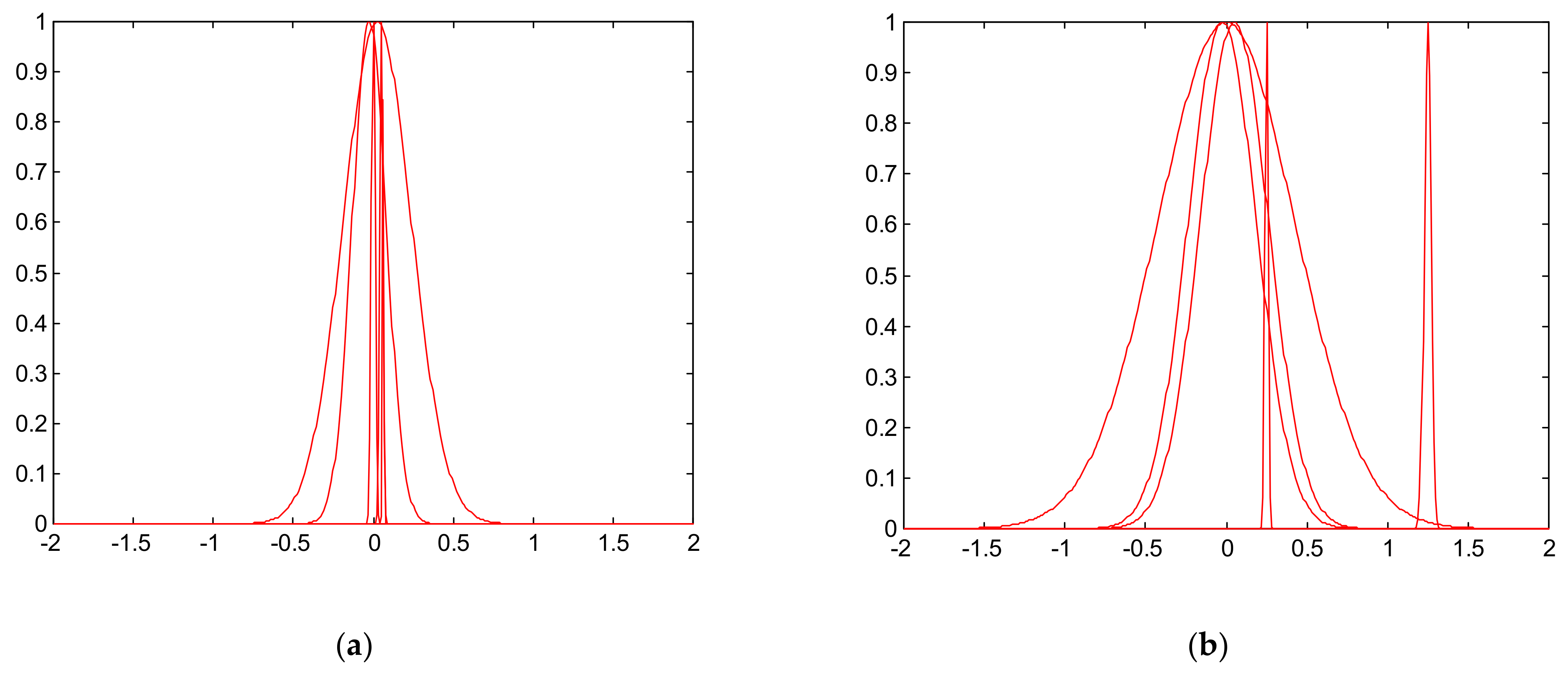
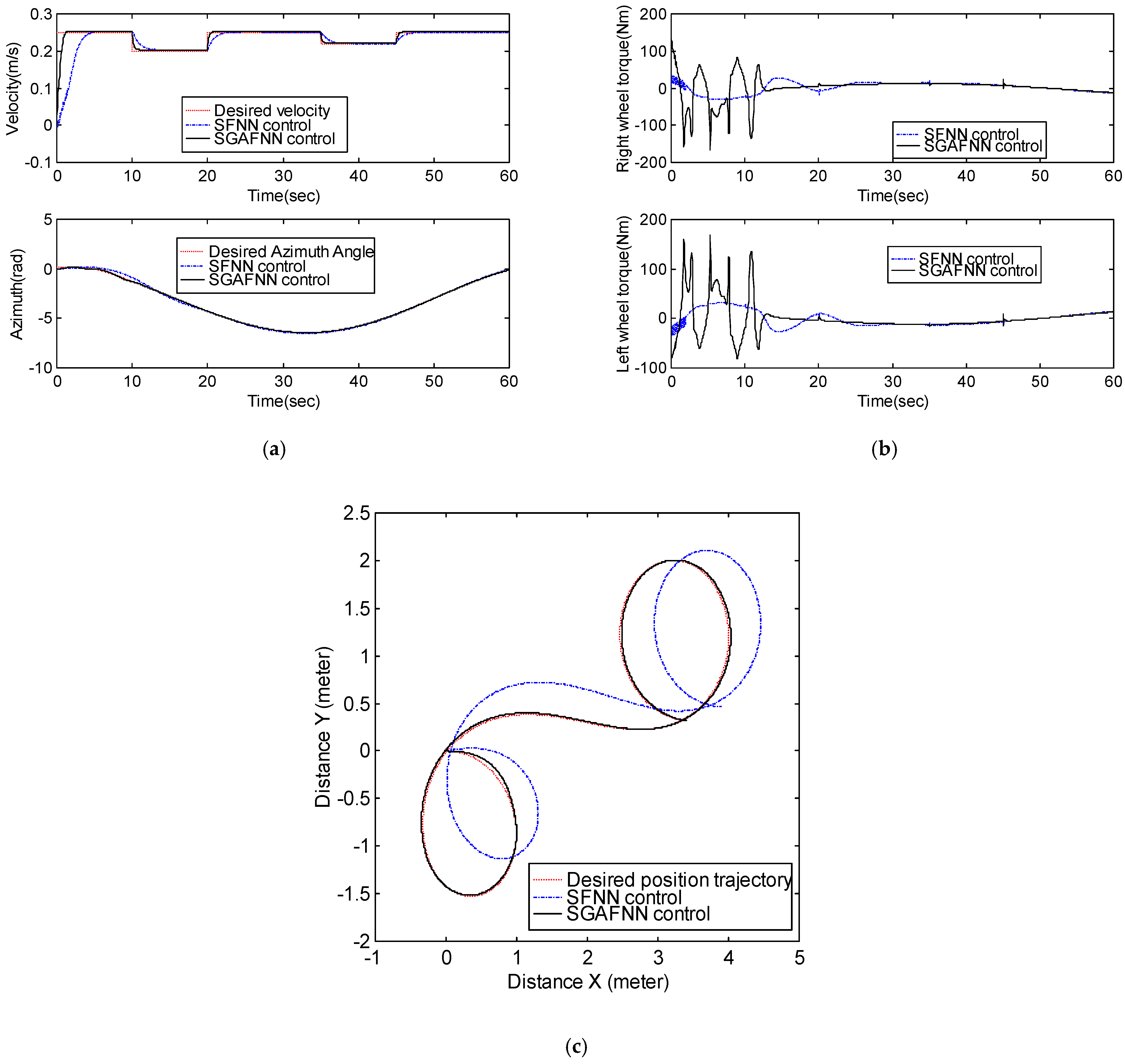
3. Simulation Result

When considering a mobile service robot model, a mathematical model can be set as shown in Figure 3. The state spaces of the dynamic equations are described as below [15]:

$$\begin{array}{l} \dot{\mathit{x}}=\mathit{Ax}+\mathit{Bu}\\ \mathit{y}=\mathit{Cx}\end{array}$$

(24)

where $\begin{array}{l}\mathit{A}=\left[\begin{array}{ccc}{\mathit{a}}_1& 0& 0\\ 0& 0& 1\\ 0& 0& {\mathit{a}}_2\end{array}\right]\\ \mathit{B}=\left[\begin{array}{cc}{\mathit{b}}_1& {\mathit{b}}_1\\ 0& 0\\ {\mathit{b}}_2& -{\mathit{b}}_2\end{array}\right]\\ \mathit{C}=\left[\begin{array}{ccc}1& 0& 0\\ 0& 1& 0\end{array}\right]\end{array}$, $\begin{array}{l}\mathit{x}={\left[\begin{array}{ccc}\mathit{v}& \mathit{\phi }& \dot{\mathit{\phi }}\end{array}\right]}^{\mathit{T}}\\ \mathit{u}={\left[\begin{array}{cc}{\mathit{u}}_{\mathit{r}}& {\mathit{u}}_{\mathit{l}}\end{array}\right]}^{\mathit{T}}\\ \mathit{y}={\left[\begin{array}{cc}\mathit{v}& \mathit{\phi }\end{array}\right]}^{\mathit{T}},\end{array}$ and $\begin{array}{c}{\mathit{a}}_1=-\frac{2\mathit{c}}{\mathit{M}{\mathit{r}}^2+2{\mathit{I}}_{\mathit{w}}}\\ {\mathit{a}}_2=-\frac{2\mathit{c}{\mathit{l}}^2}{{\mathit{I}}_{\mathit{v}}{\mathit{r}}^2+2{\mathit{I}}_{\mathit{w}}{\mathit{l}}^2}\\ {\mathit{a}}_3=\frac{\mathit{k}\mathit{r}}{\mathit{M}{\mathit{r}}^2+2{\mathit{I}}_{\mathit{w}}}\\ {\mathit{a}}_4=\frac{\mathit{k}\mathit{r}\mathit{l}}{{\mathit{I}}_{\mathit{v}}{\mathit{r}}^2+2{\mathit{I}}_{\mathit{w}}{\mathit{l}}^2}\end{array}$.

The detail meanings of the parameters can be found in [15].

An SGAFNN is designed to control the robot. The design purpose is to force the robot to track a desired path, which is obtained from the image of the camera and data from ultrasound sensors, the purpose of which is to decide whether the velocity should be down or not and how much the turning angle should be changed so as to avoid collisions with obstacles and walls. The real design environment diagram is as Figure 4. The velocity will be down when the obstacle image is obtained from the camera and the turning angle is tuned to avoid collision.

The input variables of SGAFNN are the tracking sliding function ${\mathit{s}}_{\mathit{v}},{\mathit{s}}_{\mathit{\phi }}$ and its derivative ${\dot{\mathit{s}}}_{\mathit{v}},{\dot{\mathit{s}}}_{\mathit{\phi }}$ of the robot’s speed ${\mathit{v}}_{\mathit{d}}$ and rotation angle ${\mathit{\phi }}_{\mathit{d}}$, and the output variable is the torque of the robot, such as obtaining the required speed ${\mathit{u}}_{\mathit{v}}$ and rotation angle ${\mathit{u}}_{\mathit{\phi }}$, respectively. The control terms of the robot are ${\mathit{u}}_{\mathit{v}}$ and ${\mathit{u}}_{\mathit{\phi }}$, and the control torques are used for the left ${\mathit{u}}_{\mathit{l}}$ and right ${\mathit{u}}_{\mathit{r}}$ wheels, for a robot with two independent drive wheels. This is based on the design concept of SGAFNN, including a GAFNN and a sliding mode control input, namely

$${{\displaystyle \mathit{u}}}_{\mathit{v}}={\mathit{u}}_{\mathrm{SGAFNN}1}+{\mathit{u}}_{\mathit{s}1}$$

(25)

$${{\displaystyle \mathit{u}}}_{\mathit{\phi }}={\mathit{u}}_{\mathrm{SGAFNN}2}+{\mathit{u}}_{\mathit{s}2}.$$

(26)

The controlled terms of robot are $\mathit{v}$ and $\mathit{\phi }$ and the control torques ${\mathit{u}}_{\mathit{l}},{\mathit{u}}_{\mathit{r}}$ are implemented to the left and right wheels. From the property of a robot with two independent driving wheels, the following relation equations are considered:

$${\mathit{u}}_{\mathit{r}}={\mathit{u}}_{\mathit{v}}+{\mathit{u}}_{\mathit{\phi }}.$$

(27)

$${\mathit{u}}_{\mathit{l}}={\mathit{u}}_{\mathit{v}}-{\mathit{u}}_{\mathit{\phi }}$$

(28)

The first step is to design the GAFNN controllers, which can tune the weightings online to force the sliding mode controller to work well such that its tracking error converges to zero in order to obtain a good tracking performance. Because the sliding mode controllers have been designed to cooperate with a GAFNN controller, the SGAFNN needs only 5 neurons in layer (D) of GAFNN, that is, 25 fuzzy rules are applied to input variables. The initial and tuned membership functions are shown in Figure 5. The weightings of $\alpha ,\beta$ are set from 0.1 to 0.5 separately. The weightings of GAFNN are adjusted by an adaptive law from (12) to (14) to make real-time online adjustments. The learning factors are all set at 0.015. The simulation sample time is 0.02 s. In the simulation, the real parameters of the robot are ${\mathit{I}}_{\mathit{v}}=10 {\mathrm{kgm}}^2$, $\mathit{M}=20 \mathrm{kg}$, $\mathit{l}=0.3 \mathrm{m}$, ${\mathit{I}}_{\mathit{w}}=0.005 {\mathrm{kgm}}^2$, $\mathit{c}=0.05 {\mathrm{kgm}}^2/\mathit{s}$, $\mathit{r}=0.1 \mathrm{m}$, and $\mathit{k}=5$. Meanwhile, the reference velocity ${\mathit{v}}_{\mathit{d}}$ is given as 0.25 m/s, but the velocity will be down because the robot faces obstacles at times of 10 s and 35 s. The initial values of states variables are given as $\mathit{x}(0)={\left[\begin{array}{ccc}0& 0& 0\end{array}\right]}^{\mathit{T}}$. The simulation results are shown in Figure 6. In the simulation of speed and direction control, although the effect of a sliding mode fuzzy neural network (SFNN) is already very good, in the sustainable development of artificial intelligence control, SGAFNN obviously improves the transient response and steady-state response; this is because, in addition to SFNN control, there are more and more complex parameters operations in SGAFNN such that it can obtain the optimal control force in advance, instead of relying solely on the control law of the SFNN control. This simulation result can also verify that the sustainable developing artificial intelligence control law is far superior to the traditional SFNN control law. By comparing the proposed design method of SGAFNN with the traditional SFNN methodology, improved and better performances and robustness are achieved.

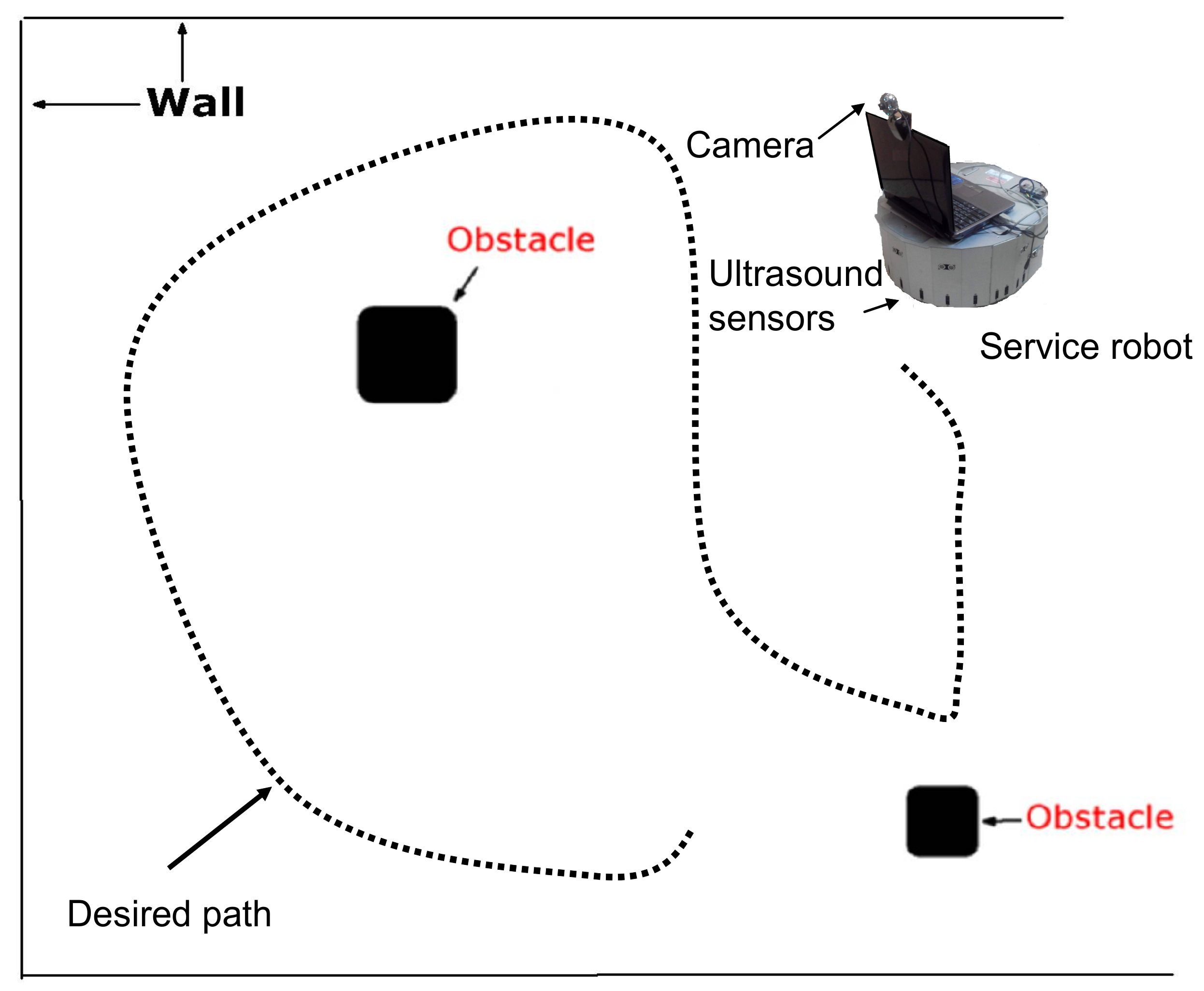
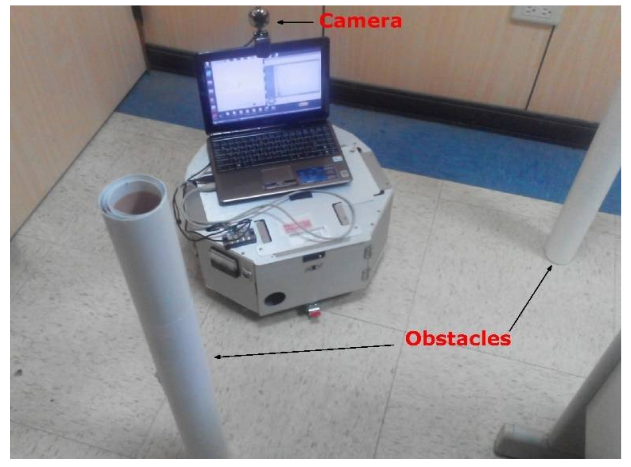
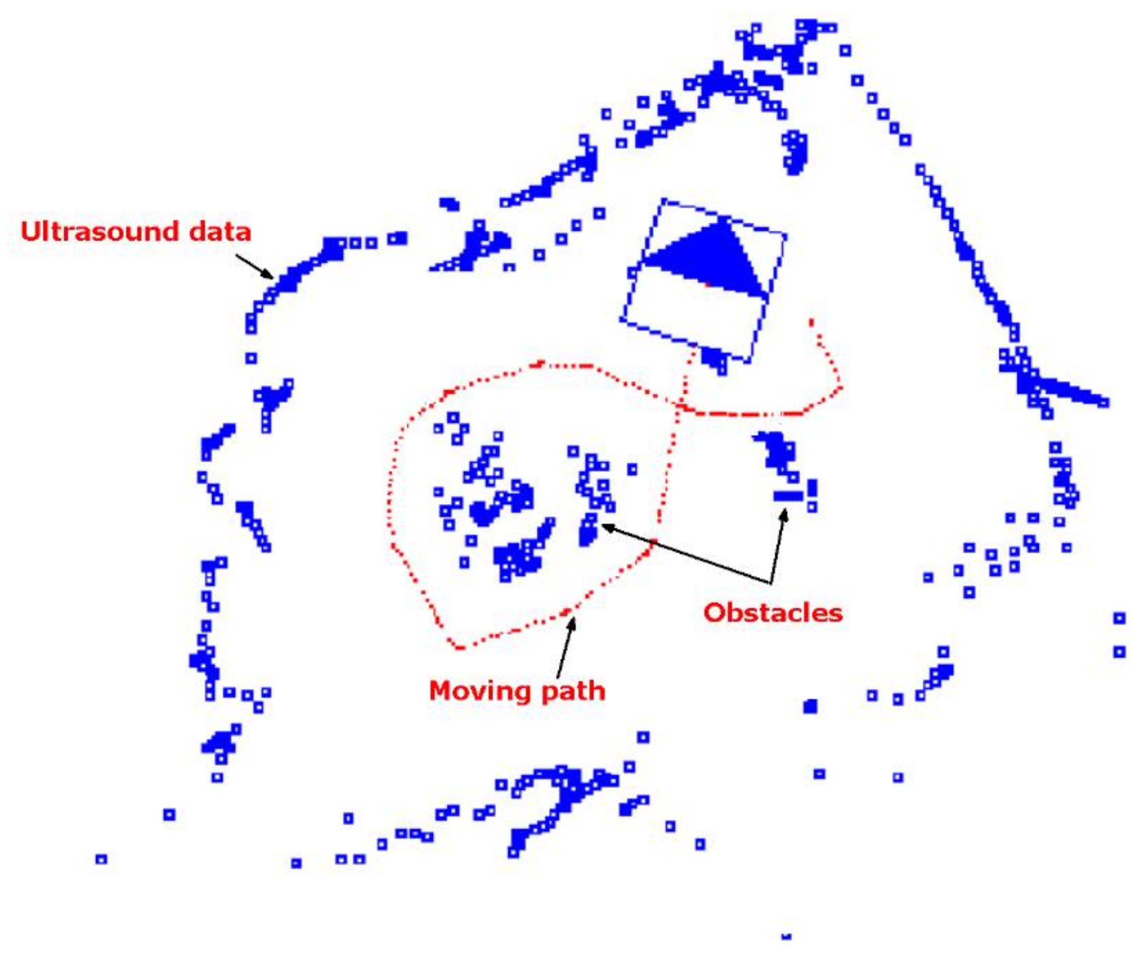
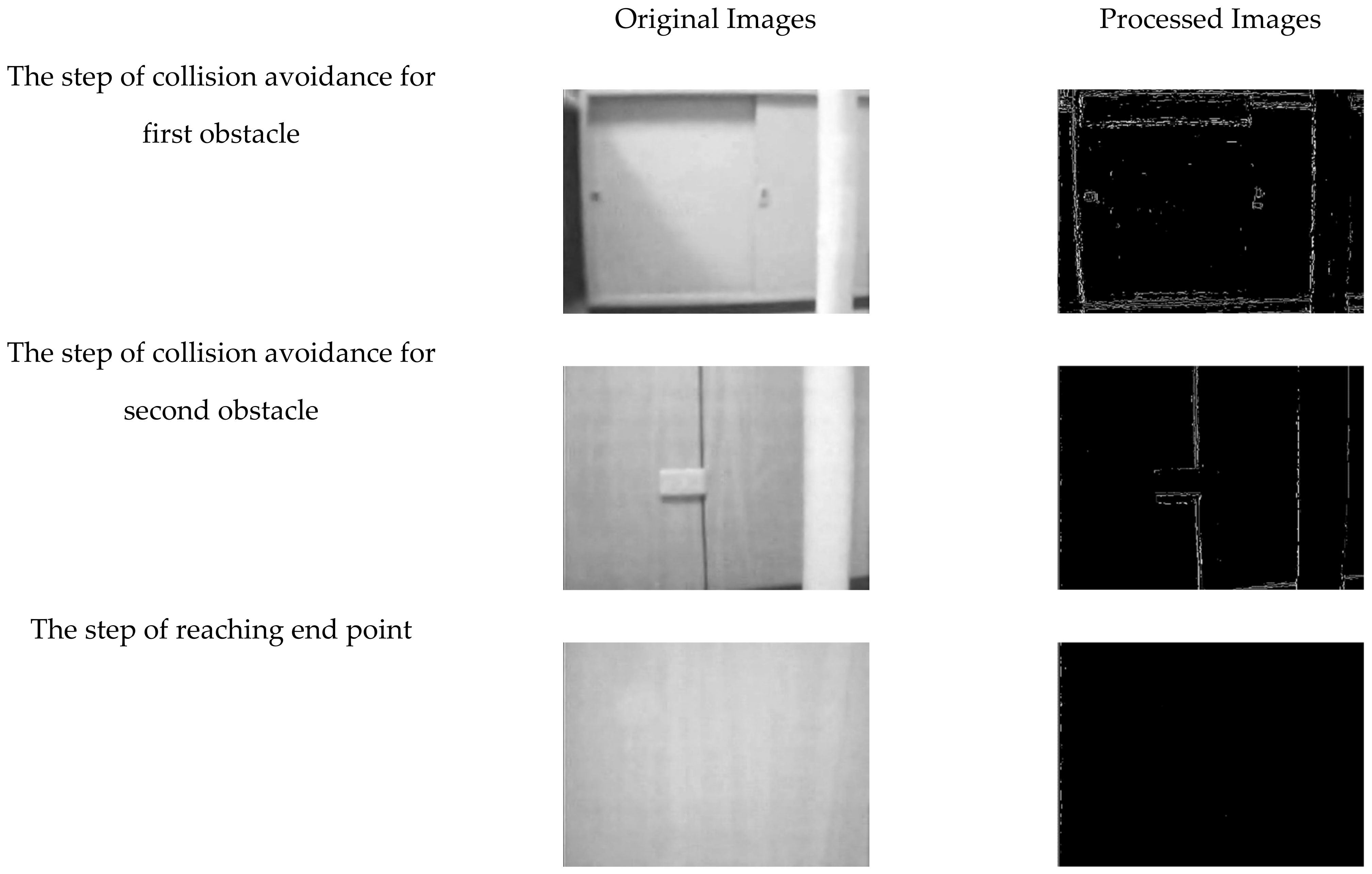
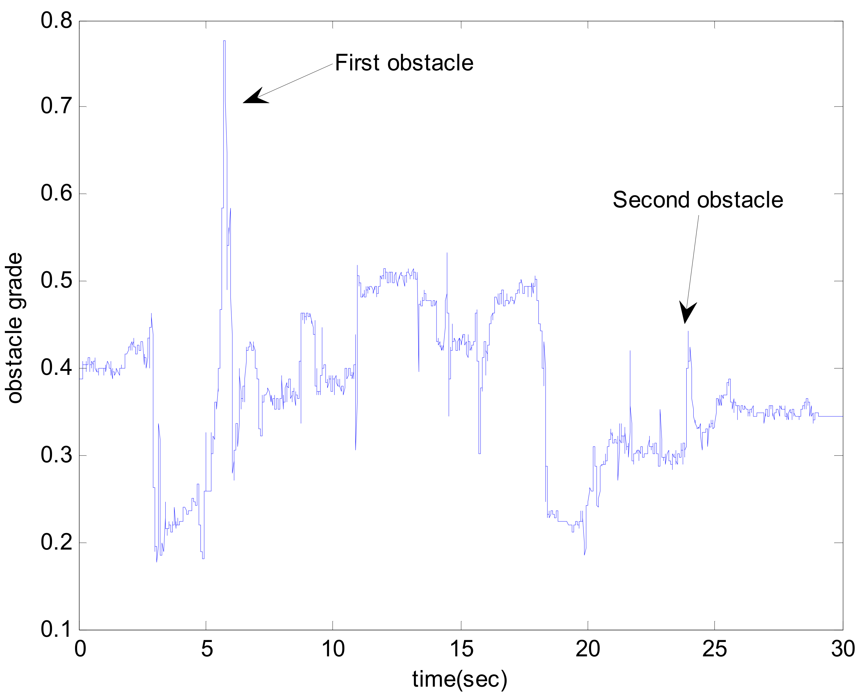
4. Practical Evaluations

The experimental robot is composed of two driving wheels, one auxiliary wheel, a DC motor, a control system, a driving system, a decoder, and software. The control board consists of a CPU with a computing speed of 150 MHz, 32 bits, and 32 K RAM. There are 11 ultrasonic sensors around to read the surrounding data. In addition, a notebook computer is used to connect to the control board via USB, process control signals, and issue commands to control the motors. Using this robot control panel and control system, signal observation and analysis for many robot controls, including position, velocity, and acceleration control, can be easily accomplished. Using sensor information and control system software, and by connecting with a laptop, many intelligent high-end robots controls can be completed, such as obstacle avoidance and path planning. In this paper, the practical test environment is set up as Figure 7. Two barriers were set up for testing. After reading the image and ultrasound sensor data, the robot can be controlled by the SGAFNN controller. The result of the motion trajectory is shown in Figure 8.

This shows that the wall and obstacles can be avoided. Regarding the image processing, results are shown in Figure 9 and Figure 10. The commonly used image edge detection technique is utilized to identify the obstacle grade signal; if it exists, the peak signal will be generatedto slow down the robot speed. Meanwhile, by using ultrasound sensors a desired path can be generated. Finally, the SGAFNN cooperates with these data to control the robot to follow this desired path. The experiment shows that the proposed SGAFNN possesses good performance in terms of velocity and turning angle control so as to avoid collision with walls and obstacles in the real test environment.

5. Conclusions

In this paper, the concept is to develop a sustainable AI research method. That is, the image control and the ultrasonic control are designed separately. The control step is divided into two parts; the first part addresses the rough problem. If the first part cannot be solved, then go to the second part for more precise path control. In the first part, The ART is used to classify direction; in the second part, the SC is combined with GAFNN to be successful as a full controller of SGAFNN. The GAFNN controller is for compensating the error between the optimized GAFNN controller and the full controller. The system stability is guaranteed. Based on the image edge detection technique, a desired path can be obtained so as to feed it to the robot to follow to avoid collision with walls and obstacles. The simulation results show that the proposed SGAFNN controller reveals better performance, robustness, and guaranteed stability compared with traditional sliding mode fuzzy neural network control. The practical implementation of a robot demonstrates that the performance of the proposed methodology is effective, reliable, and good.

References

1. Carpenter, G.A.; Grossberg, S. ART 2: Self-organization of stable category recognition codes for analog input patterns. Appl. Opt. 1987, 26, 4919–4930. [Google Scholar] [CrossRef] [PubMed]
2. Petridis, V.; Kaburlasos, V. Fuzzy Lattice Neural Network (FLNN): A hybrid model for learning. IEEE Trans. Neural Netw. 1998, 9, 877–890. [Google Scholar] [CrossRef] [PubMed]
3. Carpenter, G.A.; Grossberg, S.; Markuzon, N.; Reynolds, J.H.; Rosen, D.B. Fuzzy ARTMAP: A neural network architecture for incremental supervised learning of analog multidimensional maps. IEEE Trans. Neural Netw. 1992, 3, 698–713. [Google Scholar] [CrossRef] [PubMed] [Green Version]
4. Massey, L. Soft-clustering and improved stability for adaptive resonance theory neural networks. Soft Comput. 2008, 12, 657–665. [Google Scholar] [CrossRef]
5. Heins, L.G.; Tauritz, D.R. Adaptive Resonance Theory (ART): An Introduction. 1995. Available online: https://www.researchgate.net/publication/247749347_Adaptive_Resonance_Theory_ART_An_Introduction (accessed on 7 April 2022).
6. Parham, N.; Loo, C.K.; Manjeevan, S. Semi-supervised topo-Bayesian ARTMAP for noisy data. Appl. Soft Comput. 2018, 62, 134–147. [Google Scholar] [CrossRef]
7. Amutha, A.L.; Annie Uthra, R.; Preetha Roselyn, J.; Golda Brunet, R. Classification of Anomalies in Multivariate Streaming Phasor Measurement Unit Data Using Supervised and Clustering Ensemble Techniques. In Proceedings of the 2021 5th International Conference on Electronics, Communication and Aerospace Technology (ICECA), Coimbatore, India, 2–4 December 2021; pp. 1460–1466. [Google Scholar]
8. Rashid, M.; Khan, M.A.; Alhaisoni, M.; Wang, S.-H.; Naqvi, S.R.; Rehman, A.; Saba, T. A Sustainable Deep Learning Framework for Object Recognition Using Multi-Layers Deep Features Fusion and Selection. Sustainability 2020, 12, 5037. [Google Scholar] [CrossRef]
9. Nalpantidis, L.; Gasteratos, A. Stereovision-based fuzzy obstacle avoidance method. Int. J. Humanoid Robot. 2011, 8, 169–183. [Google Scholar] [CrossRef]
10. Mon, Y.J. WSN-based indoor location identification system (LIS) applied to vision robot designed by fuzzy neural network. J. Digit. Inf. Manag. 2015, 13, 39–44. [Google Scholar]
11. Wang, H.; Ren, Y.; Meng, Z. A Farm Management Information System for Semi-Supervised Path Planning and Autonomous Vehicle Control. Sustainability 2021, 13, 7497. [Google Scholar] [CrossRef]
12. Das Sharma, K.; Chatterjee, A.; Rakshit, A. A PSO—Lyapunov Hybrid Stable Adaptive Fuzzy Tracking Control Approach for Vision-Based Robot Navigation. IEEE Trans. Instrum. Meas. 2012, 61, 1908–1914. [Google Scholar] [CrossRef]
13. Mon, Y.J. Machine vision based sliding fuzzy-PDC control for obstacle avoidance and object recognition of service robot platform. J. Intell. Fuzzy Syst. 2015, 28, 1119–1126. [Google Scholar] [CrossRef]
14. DeSouza, G.; Kak, A. Vision for mobile robot navigation: A survey. IEEE Trans. Pattern Anal. Mach. Intell. 2002, 24, 237–267. [Google Scholar] [CrossRef] [Green Version]
15. Watanabe, K.; Tang, J.; Nakamura, M.; Koga, S.; Fukuda, T. A fuzzy-Gaussian neural network and its application to mobile robot control. IEEE Trans. Control Syst. Technol. 1996, 4, 193–199. [Google Scholar] [CrossRef]
16. Mon, Y.J.; Lin, C.M. Supervisory fuzzy Gaussian neural network design for mobile robot path control. Int. J. Fuzzy Syst. 2013, 15, 142–148. [Google Scholar]
17. Hmoud Al-Adhaileh, M.; Waselallah Alsaade, F. Modelling and Prediction of Water Quality by Using Artificial Intelligence. Sustainability 2021, 13, 4259. [Google Scholar] [CrossRef]
18. Li, Z. Tension control system design of a filament winding structure based on fuzzy neural network. Eng. Rev. 2015, 35, 9–17. [Google Scholar]
19. David, J.; Brom, P.; Starý, F.; Bradáč, J.; Dynybyl, V. Application of Artificial Neural Networks to Streamline the Process of Adaptive Cruise Control. Sustainability 2021, 13, 4572. [Google Scholar] [CrossRef]
20. Nguyen, T.-B.-T.; Liao, T.-L.; Yan, J.-J. Adaptive Sliding Mode Control of Chaos in Permanent Magnet Synchronous Motor via Fuzzy Neural Networks. Math. Probl. Eng. 2014, 2014, 868415. [Google Scholar] [CrossRef] [Green Version]
21. Wang, H.; Zhou, Q.; Yang, X.; Karimi, H.R. Robust Decentralized Adaptive Neural Control for a Class of Nonaffine Nonlinear Large-Scale Systems with Unknown Dead Zones. Math. Probl. Eng. 2014, 2014, 841306. [Google Scholar] [CrossRef] [Green Version]
22. Seshagiri, S.; Khalil, H.K. Output feedback control of nonlinear systems using RBF neural networks. IEEE Trans. Neural Netw. 2000, 11, 69–79. [Google Scholar] [CrossRef] [Green Version]
23. Owens, D.H. Iterative Learning Control: An Optimization Paradigm; Springer: Cham, Switzerland, 2015; ISBN 978-1-4471-6772-3. [Google Scholar]
24. Wang, L.X. Adaptive Fuzzy Systems and Control: Design and Stability Analysis; Prentice-Hall: Englewood Cliffs, NJ, USA, 1994; pp. 140–154. [Google Scholar]
25. Slotine, J.-J.E.; Li, W.P. Applied Nonlinear Control; Prentice-Hall: Englewood Cliffs, NJ, USA, 1991. [Google Scholar]
26. Wu, L.; Su, X.; Shi, P. Sliding mode control with bounded L2 gain performance of Markovian jump singular time-delay systems. Automatica 2012, 48, 1929–1933. [Google Scholar] [CrossRef]
27. Li, F.; Wu, L.; Shi, P.; Lim, C.-C. State estimation and sliding mode control for semi-Markovian jump systems with mismatched uncertainties. Automatica 2015, 51, 385–393. [Google Scholar] [CrossRef]
28. Delavari, H. A novel fractional adaptive active sliding mode controller for synchronization of non-identical chaotic systems with disturbance and uncertainty. Int. J. Dyn. Control 2017, 5, 102–114. [Google Scholar] [CrossRef]
29. Li, H.-R.; Jiang, Z.-B.; Kang, N. Sliding Mode Disturbance Observer-Based Fractional Second-Order Nonsingular Terminal Sliding Mode Control for PMSM Position Regulation System. Math. Probl. Eng. 2015, 2015, 370904. [Google Scholar] [CrossRef] [Green Version]
30. Rahman, N.; Lee, M.C. Actual reaction force separation method of surgical tool by fuzzy logic based SMCSPO. Int. J. Control. Autom. Syst. 2015, 13, 379–389. [Google Scholar] [CrossRef]
31. Bajrami, X.; Pajaziti, A.; Likaj, R.; Shala, A.; Berisha, R.; Bruqi, M. Control Theory Application for Swing Up and Stabilisation of Rotating Inverted Pendulum. Symmetry 2021, 13, 1491. [Google Scholar] [CrossRef]
32. Li, J.; Zhang, Y.; Jin, Z. The Approximation of the Nonlinear Singular System with Impulses and Sliding Mode Control via a Singular Polynomial Fuzzy Model Approach. Symmetry 2021, 13, 1409. [Google Scholar] [CrossRef]
Figure 1. The diagram of GAFNN.
Sustainability 14 05335 g001
Figure 2. The design concept block diagram of SGAFNN control for service robot.
Sustainability 14 05335 g002
Figure 3. O-XY plane diagram of robot.
Sustainability 14 05335 g003
Figure 4. The diagram of real practical test for robot.
Sustainability 14 05335 g004
Figure 5. (a). Initial membership functions of SGAFNN for velocity. (b). Adaptive membership functions of SGAFNN for velocity.
Sustainability 14 05335 g005
Figure 6. (a). System states trajectories of SGAFNN. (b). Control inputs of SGFNN. (c). Moving path diagram of robot.
Sustainability 14 05335 g006
Figure 7. The set-up diagrams of practical implementation for robot.
Sustainability 14 05335 g007
Figure 8. The ultrasound sensed diagrams for robot moving.
Sustainability 14 05335 g008
Figure 9. The image edge processing diagrams of practical implementation for robot moving.
Sustainability 14 05335 g009
Figure 10. The result diagram of image edge processing of practical implementation for robot moving.
Sustainability 14 05335 g010