Article

Freight Transport Cost and Urban Sprawl across EU Regions

by
Theodore Tsekeris
1,2
1
Centre of Planning and Economic Research (KEPE), 10672 Athens, Greece
2
School of Public Leadership, Stellenbosch University, Stellenbosch 7599, Western Cape, South Africa
Sustainability 2022, 14(9), 5217; https://doi.org/10.3390/su14095217
Submission received: 1 March 2022 / Revised: 21 April 2022 / Accepted: 25 April 2022 / Published: 26 April 2022

Abstract

:
This paper investigates the impact that urban sprawl and land use patterns have on freight transport costs at the regional level in Europe. A unique dataset is employed, which distinguishes various aspects of freight transport costs across EU regions. The measurement of sprawl metrics is based on the European soil sealing (artificial land cover) data concerning the land uptake for buildings and related infrastructure, as well as land use data originating from the Land Use/Cover Area frame Survey of Eurostat. The econometric analysis indicates that both the increased scale and compact development of land for urban settlement and specific (industrial, services/residential) activities can significantly reduce average road freight transport costs. The increased land use mixture and the share of industrial activity also have a negative impact on road freight transport costs. The results highlight the importance of integrated spatial/land use planning policies to manage freight transport costs and improve the sustainable urban development of EU regions.

1. Introduction

The freight transport cost constitutes a crucial element of the productivity and growth of firms, regions, and countries, as it directly affects the proximity and connectivity of economic activity across space, as well as the import and export performance and competitiveness. The two basic variables of transport cost refer to the network distance and travel time. According to the Eurostat transport statistics, road transport is the dominant mode of freight movement, covering, on average, during 2010–2018, about 76% of the total inland freight transport (in tonne-kilometres) in the EU. Based on the EUREGIO’s interregional intersectoral input–output database [1], in 2010, 52% of the total trade in the EU took place in relatively short distances, within regions, compared to interregional trade. In the short-distance freight transport, trucks are by far the most competitive mode in the EU (with a modal split of more than 80% for trips shorter than 150 km), while the share of commodities moved by truck falls as the trip distance increases [2].
The increased amount of network distance travelled by truck vehicles is usually associated with more energy fuel consumption, environmental pollution, road traffic accidents, investment in road infrastructure supply, maintenance and repair, and other negative externalities. In addition, longer road transport distances and longer travel times typically lead to reduced regional accessibility and increased road traffic congestion. Hence, the regional analysis of road freight transport cost can provide us with useful insights about its influencing factors and the sustainable development of transport/logistics infrastructure and services.
The road freight transport cost depicts, in some way, the space and time separation among various stages of the supply chain, e.g., from the arrival at ports and the places of agricultural production and raw material extraction to intermediate/final goods processing plants, warehouses/distribution centres, and points of delivery to customers. Increased transport distances and travel times at the regional level have often been attributed to the diffusion of urban or built-up area development, referred to as sprawl, due to either various market mechanisms or the (unintended) outcome of government interventions to regulate and/or restrict land consumption [3,4]. However, the impact of urban sprawl and land use patterns on transport costs has been largely examined in relation to commuting (home-to-work travel) distances and times, compared to the corresponding implications for freight transport, which remain an overlooked topic.
The main objective of this paper is to investigate the impact of urban sprawl on the average generalised freight transport cost and its components (transport distances and travel times) across EU regions. For this purpose, different sprawl metrics are employed, including the percentage of built-up area, the land uptake per person, the degree of urban dispersion, the weighted urban proliferation, and the land use density for housing and services, and for industrial activities, and the land use mix. The next section provides an overview of the role that urban sprawl/land use patterns and other regional variables play in the cost structure of freight transport; Section 3 describes the specification of the econometric model and its variables; Section 4 presents and discusses the empirical results; and Section 5 summarises and concludes the major findings of the paper.

2. Regional Freight Transport and Spatial Structure

There is well-established scholarly literature on the land use factors that influence transport. [5] theoretically considered spatial/land use planning and transport planning as two parallel types of planning, which interact with each other and should be coordinated at the subregional, regional, and national levels, and he proposed a model that utilises land use data as the input for predicting transport demand and cost measures. Other processes, such as those of economic (industrial) planning, may also be encountered in this comprehensive modelling framework. The theoretical background and empirical testing of the land use impacts on transport output and travel behaviour have been examined in several studies, principally through the consideration of factors related to the density, mixing, design, and accessibility (in terms of easiness of reaching or proximity) of land uses [6,7].
Specifically, with regard to the linkage of freight transport costs with the spatial structure at the regional level, this is primarily driven by the space–time pattern of connectivity among the various trade (supply and demand) locations. Hence, it can be regarded as a composite result of the size, proportion, and dispersion of the various land uses and the built-up area over the landscape of a region. Namely, both the characteristics of land cover and land uses may significantly affect different dimensions of the average freight transport costs. However, an empirical investigation of the relationship between urban sprawl or land uses and transport costs has largely focused on the impacts on commuting, particularly in urban areas [6,7,8,9,10,11], rather than on freight transport, and in the regional context.
Specifically, Ref. [12] found that the separation between the location of several UK urban areas with commercial and industrial centres positively influences the average distances over which goods are moved. Other relevant studies have focused on analysing the significant—albeit heterogeneous—impact of built environment variables at the level of urban areas, such as the urban population/employment density and land use mix, on urban freight transport in the context of trip generation and trip attraction models [13,14,15,16].
Additionally, less urban sprawl, which can be expressed as a smaller land uptake, in terms of the built-up area per capita, and/or less developed land per capita for various socio-economic purposes, entail fewer marginal costs of infrastructure and network service provision. Furthermore, the containment of sprawl can possibly promote the implementation and effectiveness of land use consolidation and the coordination of regional development plans [17]. In addition to efficiency gains, compact regional development has been found to reduce carbon emissions from transport [18], to prevent the loss of biodiversity [19] and to retain the amount of land for agricultural and forestry uses. The increased proportion of built-up areas in some regions implies a smaller proportion of agricultural land and forest and natural vegetated areas.
Nonetheless, in many circumstances, it can be argued that compact development cannot efficiently match the regional spatial structure to travel needs and it raises land prices, while restrictive land use regulations or anti-sprawl policies to make an urbanised region more compact may lead to other ones becoming more sprawled [3,20]. This is because, in some cases, the negative effects of expansive land developments in a region may be cancelled out by other positive effects on economic growth; for instance, due to the construction itself, the (temporary) alleviation of traffic congestion, the reduction in property prices, and the attraction of firms that require much space. Firms can also benefit from the substitution of land for labour at suburban locations, making labour units more productive and—to some extent—compensating for productivity loss due to weakened agglomeration economies. This is because, in those locations where developed land per capita is higher, land rent prices are cheaper, wages for workers are lower, and firms can charge higher prices to customers who avoid congestion when they travel [3,4].
The scale of urbanisation is also considered as affecting average freight transport costs, as the expansion of urbanisation (built-up area) can be associated with agglomeration economies and a polycentric form of development, through the formation of activity clusters in the region. Such forms of urbanisation can arguably better contain travel demands and decrease transport distances, compared to a compact monocentric development [20,21]. Particularly, it is argued that population growth leads to a more dispersed and polycentric organisation of economic activity patterns, so that firms and consumers offset the adverse impact of increasing congestion, which, in turn, leads to shorter travel distances [22,23].
Other factors influencing the average freight transport cost encompass economic (industrial) composition effects, as the larger proportion of industrial activity can be related to larger manufacturing firms and, hence, the need for more space, better infrastructure services and improved freight transport by truck [24], and the operation of large seaports, which function as import–export nodes, facilitating both domestic and foreign trade flows from/to a specific region. In the latter case, depending upon the characteristics of the region, the type and the intensity of the maritime activity, sea gateways, on the one hand, may cause a larger agglomeration of logistics patterns, but, on the other hand, may induce a higher decentralisation or de-concentration of warehousing and distribution facilities and freight transport flows, compared to the geographical spread of the regional population or employment [25].
This paper describes a comprehensive econometric model for representing the impact that various aspects of urban sprawl and land use patterns have on the generalised average freight transport cost and its components at the EU regional level. The contributions of this paper to the scholarly literature and the empirical research relate to identifying the diverse impact that urban sprawl and land use patterns have on freight transport cost. This task has been largely overlooked in the current literature due to the complicated nature of land use and freight/goods distribution, and the lack of reliable or good-quality data on both freight cost and land use at the macro scale, such as the level of EU regions. The land cover/urban sprawl factors considered here include the percentage of the built-up area, the land uptake per person, the degree of urban dispersion, and the composite measure of weighted urban proliferation. The land use factors include the density of land for services and residential purposes, and for industrial and construction activities, as well as the land use mixture. The multitude of results of the present analysis allows us to obtain insights into the existence and extent of the possibilities for managing freight transport via land use policies.
As it is shown in Table 1, the proposed model examines the whole range of land use and urban sprawl variables, which have been hitherto considered in the existing scholarly literature, except for the design dimensions of the built environment, such as the design of building blocks, pedestrian-oriented facilities, streets and parking facilities, and the accessibility of land uses, which are practically impossible to measure in detail for all urbanised areas at the European scale. At the same time, the model encompasses a range of other (control) factors, which can positively or negatively affect the average freight transport costs, such as the scale of urbanisation, the economy (industrial composition), and the transport geography and performance (seaport throughput) of regions. Detailed explanations about the definition of variables and the model specification are presented in the next section. Lastly, Figure 1 illustrates a task diagram, including the data and method used in the study, so that it offers a comprehensive picture of how different variables are employed and positioned in the proposed analytical/modelling framework.
Table 1. Land use/cover variables that affect (freight) transport costs and the related bibliography.
VariablesIndicative BibliographyIncluded
Land cover/urban sprawl
Proportion of built-up area[26]
Land uptake per person[17,26]
Urban dispersion[24,26]
Weighted urban proliferation[26]
Land use
Residential/commercial density[12,13,14,15,16,17,24,25]
Industrial/construction density[12]
Land use mix[13,14,17]
Accessibility (land use proximity)[13]
Built environment designs[27,28]
Notes: () and (✘) denote variables examined and not examined in the proposed model, respectively.

3. Model Specification and Description of the Variables

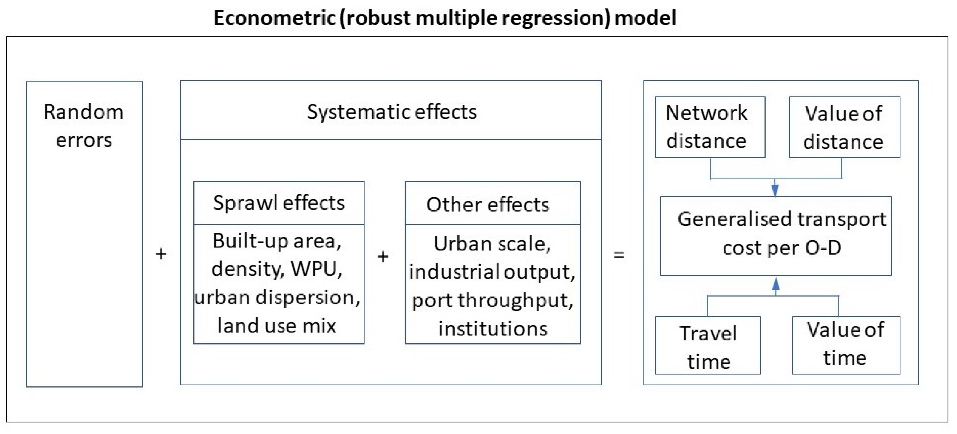
3.1. Specification of the Model

Based on the theoretical aspects and empirical evidence previously mentioned, an econometric model to represent the impact of urban sprawl/land use patterns on average road freight transport costs TCij in a region i and country j can be specified as follows:
T C i j = β 0 + β 1 s p r a w l i j + β 2 l a n d m i x i j + β 3 u r b a n i j + β 4 i n d u s t r y i j + β 5 p o r t i j + β 6 e a s t i + u j + ε i j  
where β0 is a constant and β are the coefficient estimates of the explanatory variables of the individual (distance and time) and the generalised road freight transport cost (GTC). The sprawl variable is alternatively expressed by a number of metrics measuring the dispersion of land cover and land uses. The landmix variable refers to the mixture of land areas covered by different land use categories. The urban variable refers to the scale of urbanisation, according to the OECD urban typology of regions concerning very large (metropolitan) cities, in terms of functional urban areas (FUAs) with more than 1 M inhabitants, based on the corresponding FUA database of Eurostat. Three typologies are identified here: FUAs between 1 and 2 million inhabitants, FUAs between 2 and 3 million inhabitants, and FUAs above 3 million inhabitants. The industry variable measures the proportion of the industrial added value to the total added value of a region, based on the regional statistics of Eurostat at the NUTS-2 level. The port variable refers to the logarithm of port traffic throughput (in tonnes) from/to each region, which also originates from the Eurostat database at the NUTS-2 level. The east dummy variable takes the value 1, if the region belongs to an eastern European country; otherwise, it takes the value of 0.
Country dummy variables uj also enter the model specification to control the time-invariant country-specific fixed effects. These effects may concern geographical characteristics, such as topography, availability of raw material-energy resources, and climate conditions, as well as macroeconomic and spatial planning and regulatory policies, e.g., in relation to the spatial organisation and competition conditions of the national transport and logistics market. Finally, εij refers to the independently and identically distributed (i.i.d.) error terms specific to each region.
The present methodology addresses a problem that often occurs in regression, known as heteroscedasticity, in which a systematic change in the variance of residuals exists. This problem causes an increase in the variance of coefficient estimates, making it much more likely for a model to yield an estimate as statistically significant when, actually, it is not. For this reason, the β coefficient estimates are determined here by solving a robust regression equation (or multiple regression with robust standard errors) using STATA software (edition 15.0), which results in standard errors that are more accurate and robust to the problem of heteroscedasticity [29,30].
The dependent variable represents the average road freight transport cost, which is regarded as mostly affected by the determinants of the distribution of population or economic activity within regions. This assumption can be considered as plausible, given that real transport costs are not expected to be significantly differentiated for short (intra-regional) distances according to the weight, volume, or specific measures, such as cooling, which must be taken during transport [31].
It is noted that there was a time lag of a few years before these transport cost tables become available (in 2019), as the territorialisation of international road freight data makes sense, only when the datasets of all reporting countries have been received [31,32]. There is also a considerable time lag between the average freight transport costs and the urban sprawl/land use, as well as the other explanatory (control) variables, which are dated back to 2009 (see Section 3.3). Hence, the possible issues of endogeneity are circumvented, given that the impact of urban sprawl or land use patterns on freight transport costs typically extends well beyond a single year. Nevertheless, the results should be interpreted with caution, since cross-regional analysis cannot capture the full long-term implications of maintaining or changing the spatial structure of regions.

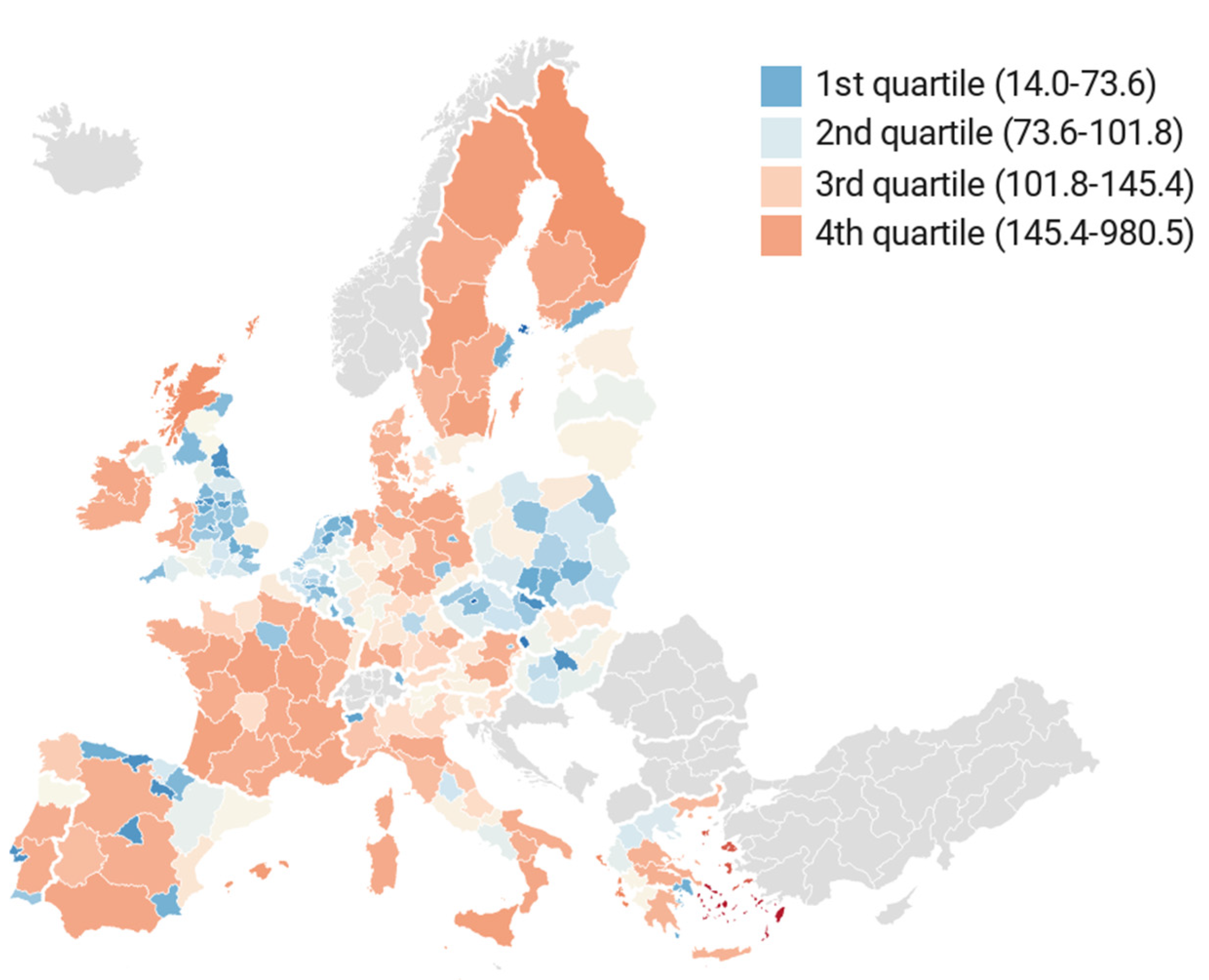
3.2. Description of the Transport Cost Variables

The current paper employs a unique transport cost dataset recently constructed and published by the Joint Research Centre of the European Commission [31,32]. In comparison to several interregional trade cost models, these transport costs have been computed both between and within the EU regions. This is because they rely on a sampling approach that allows the precise calculation of the average road freight transport costs along the optimal routes of all possible combinations of centroids obtained from a high resolution 1 km × 1 km population grid, making use of the digitalised network of OpenStreetMap, which contains an up-to-date network for roads and ferries reflecting the actual state of the European road and coast-wise transport conditions. Namely, the estimated transport costs among origin–destination centroids do not directly or indirectly assume any prior relationship with the variables used in this study, except for the existence of populations in each grid.
The average GTC of each region is weighted across all possible destinations by the GDP of each region, and assumes that road freight firms minimise the economic costs in providing transport services for any origin–destination market. The GTC combines distance- and time-related economic costs by accounting for the changes, on the one hand, in transport operating costs, i.e., fuel prices and road toll charges, and, on the other hand, institutional/regulatory conditions, related to wages in the labour market. The average GTC refers to the total estimated average cost of driving a representative 40-tonne articulated truck and it is calculated as the arithmetic mean of all distance-based and travel time-based economic costs.
By and large, the GTC reflects sources of comparative advantages across regions caused either by higher market integration and accessibility to the road network or by lower time-related costs. Figure 2 illustrates the existence of a core–periphery structure in the geographical distribution of the GTC, both within countries (capital vs. peripheral regions) as well as between them across the EU, as a result of the spatial differences in travel time and network distances, since remote regions are characterised by higher transport costs.
Specifically, the core of Europe (regions in Benelux, Germany, and southeastern UK) is characterised by low transport costs, which can be associated with positive scale economies. Relatively low transport costs are also found in most of the eastern EU regions, which appear to benefit from low transport costs, due to low time costs (wages), despite the lower levels of infrastructure endowment. Additionally, large capital (metropolitan) regions, such as those of Ile de France (Paris metropolitan area) in France, the Madrid metropolitan area in Spain, Attiki (Athens metropolitan area) in Greece, or even Stockholm in Sweden, and Helsinki in Finland, have significantly lower transport costs compared to the other peripheral regions of their own countries (Figure 2), signifying the substantial heterogeneity underlying the average transport costs across Europe. Table 2 shows the descriptive statistics of transport cost variables and their determinants. Additionally, Table 3 presents the matrix of correlation among the explanatory variables of the model. The elements of the correlation matrix are derived by calculating the measure of Pearson’s pairwise (product moment) correlation coefficient [33], through consecutively selecting each pair of continuous explanatory variable included in the models under investigation (for some introductory mathematical explanations and example estimations using STATA software, see [30]). The outcome of the correlation matrix suggests that no serious problem of multicollinearity exists, as, for all the models, the correlation coefficient between the explanatory variables does not exceed 26% (or −0.260).

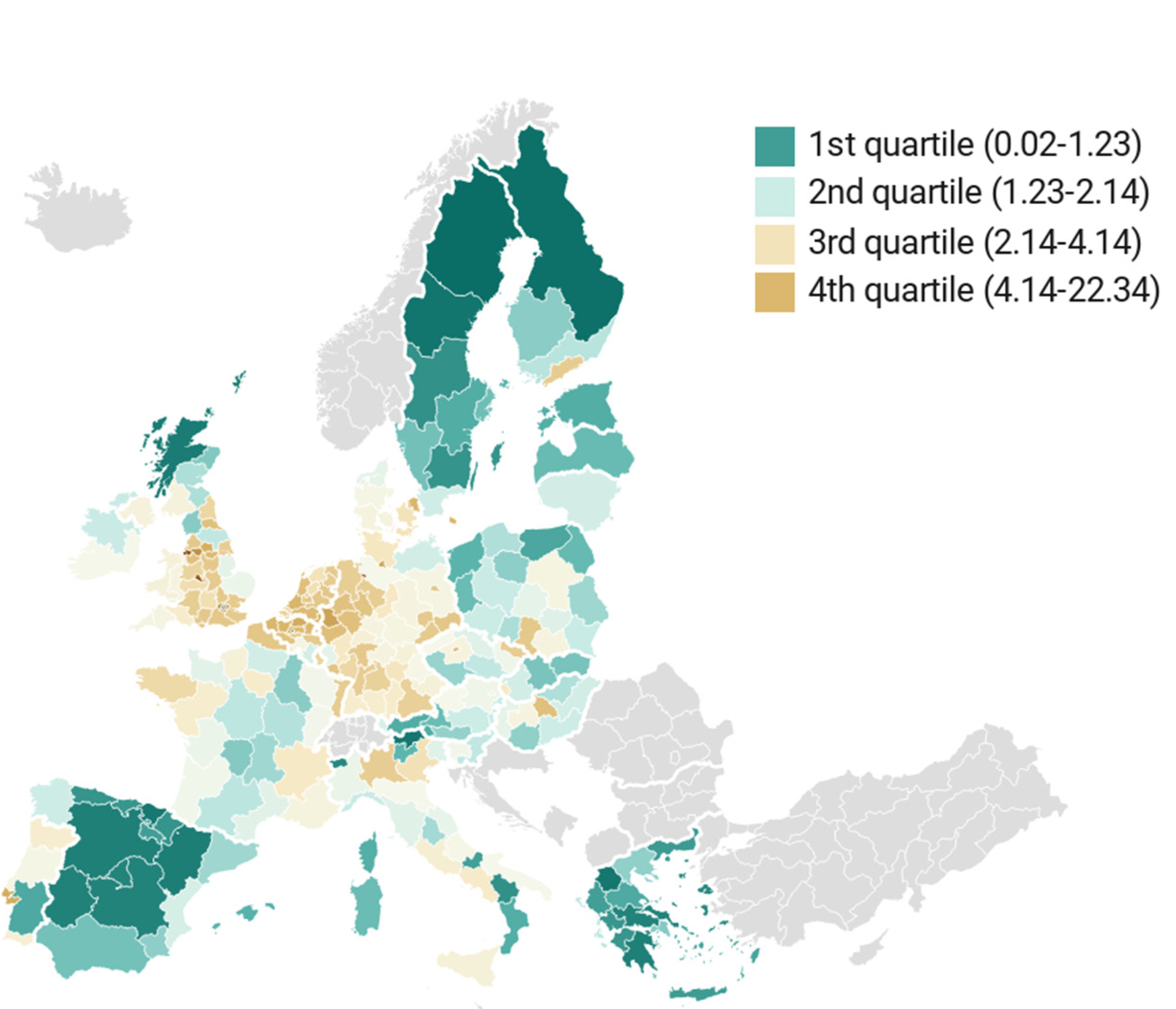
3.3. Description of the Sprawl Metrics

The measurement of sprawl is based on two sets of indexes, which correspond to different databases. The first database refers to the European soil sealing (or artificial land cover) data, which corresponds to the land uptake for buildings and related infrastructure facilities [26]. They are obtained from the Pan-European High Resolution Layer of Imperviousness Degree (HRL IMD) and consist of 20 m × 20 m pixels produced from satellite imagery for all available (continental) European NUTS-2 regions in the year 2009. Specifically, we used a balanced panel dataset, which included variables corresponding to 245 regions (at the NUTS-2 level) of 23 EU countries. In this database, the built-up areas are identified using information provided by the European Copernicus programme about all artificially sealed areas. The second database corresponds to the Land Use/Cover Area frame Survey (LUCAS) of Eurostat, which encompasses harmonised data for various land uses in the EU regions (the present data also refer to the year 2009).
It is noted that the current dataset does not come without objections, given that urban sprawl data are rather old, namely, they are only available for the year 2009, and the level of spatial analysis corresponds to the NUTS-2 level of the EU region. Nevertheless, the current dataset still constitutes a unique and sufficient database for examining the European-wide impact of urban sprawl on regional freight transport costs, considering different types of sprawl and categories of land uses, which may involve both positive and negative effects. It is also stressed that, although the data for land cover/use focusing on urban sprawl refer to the year 2009, the way of using such spatial data for environmental assessment purposes has not significantly changed over the past years [34]. The possible directions for obtaining updated data concerning urban sprawl/land use variables are discussed in the final section of the paper.

3.3.1. The Land Cover Metrics of Sprawl

These metrics concern the characteristics of the morphological structure or the land cover of urban areas, as the setting in which human action takes place, in relation to artificial constructions (mainly, built-up areas) covering the land surface [26].
The percentage of built-up areas (PBAs) is the ratio of the size of the built-up areas to the size of the total area of the reporting unit (NUTS-2 region) and is given as a percentage. It measures how large the built-up areas are (in % of the landscape). Values for landscapes of differing sizes can be directly compared because PBA is an intensive metric, i.e., the value does not depend on the size of the landscape. Given that B A is the total built-up area (in m2) and A is the total area (in m2) of a region, then:
P B A = 100 × B A A
Land uptake per person (inhabitants P and jobs J ) (LUP) describes the use of urban built-up area B A in a NUTS-2 region by people working and living in that area (m2 per inhabitant/job), as follows:
L U P = B A ( P + J )
It is noted that the inverse of this metric represents the utilisation density (inhabitants/jobs per km2), in terms of the spatial concentration of people living or working in a built-up area. Based on this definition, built-up areas with a lot of inhabitants and workers are considered to be better (more efficiently) used and, accordingly, to be less sprawled, as the ratio of inhabitants/jobs to km2 increases, given that the total area of the region is considered as fixed [17].
The degree of urban dispersion (DIS) characterises the settlement pattern in a geometric perspective and is based on the distances D i j between any two origin–destination points i j   within built-up areas (average taken over all possible pairs of points, N p , up to a maximum distance called the horizon of perception), as follows:
D I S = i j D i j / N p B A
The farther apart any two points, the higher their contribution to dispersion. In this way, the measure of D I S allows us to take into account the heterogeneity of the use of urban built-up areas within each territorial unit. This metric is expressed in urban permeation units (UPUs) per m2 of built-up area ( B A ). The UPU is a measure of the permeation of a region’s landscape by built-up areas. It can be assumed that the DIS grows with increasing population density as the buildings spread in the region, resulting in a decrease in urban sprawl and the transformation of suburban areas to urban ones [26].
Weighted urban proliferation (WUP) is a composite index (in UPU/m2) of urban sprawl, which is composed of three components: the percentage of built-up areas, the dispersion of the built-up areas, and land uptake per person (Figure 3). The WUP is based on the following definition of urban sprawl: the more area built over in a given landscape (amount of built-up area) and the more dispersed this built-up area in the landscape (spatial configuration), and the higher the uptake of the built-up area per inhabitant or job (lower utilisation intensity in the built-up area), the higher the degree of urban sprawl (for some region i and country j):
W U P = P B A × D I S × w 1 ( D I S ) × w 2 ( L U P )
Dispersion is weighted by the w 1 ( D I S ) function to make those parts of the landscape in which built-up areas are more dispersed more clearly perceived, i.e., w 1 ( D I S ) > 1 , while compact settled areas are multiplied by a lower weighting, i.e., w 1 ( D I S ) 1 . Accordingly, the metric includes a weighting factor, w 2 ( L U P ) , which is always less than 1. If the L U P is larger than 250 m2/inhabitant or job, the w 2 ( L U P ) is close to 1. If it is less than 100 m2/inhabitant or job (e.g., in city-centre areas), the w 2 ( L U P ) is close to 0 because such areas are not considered to be sprawled. Population and employment data were obtained from Eurostat at the EU NUTS-2 level of regions.
The WUP approach captures all types of settlements through the combination of its three components, so that it provides the degree of urban sprawl of the landscape in relation to the area that is potentially suitable for construction. Hence, it measures a rather complex phenomenon in a relatively simple way [35]. Specifically, Figure 3 illustrates that countries in southern Europe tend to have lower WUP index values, as they have more compact built-up areas and lower LUPs to increase shade, compared to central-western European countries, such as the Benelux countries, as well as regions in Germany and the UK (except for northern regions and inner London, which are found to be the least sprawled regions). Topographic and climatic conditions (e.g., lower WUP index values in Scandinavian countries), a history of industrialisation, socio-cultural characteristics, and institutional regimes (such as the centralised spatial-planning process in eastern EU countries, which also have lower WUP index values) affect the geographical distribution of sprawl patterns across Europe.

3.3.2. The Land Use Metrics of Sprawl

Land use metrics refer to the socio-economic activities corresponding to certain types of land use categories, such as services and residential purposes, industrial uses, agriculture, and forestry. The first land use metric refers to the sprawl of housing and services (RSS) (in m2/inhabitant-job) and is defined by the following ratio:
R S S = A R S S ( P + J S S )
where A R S S is the developed land area (in m2) occupied for services and residential purposes, P is the number of inhabitants, and J S is the number of jobs in the services sector in the region.
The second land use metric refers to the sprawl of industrial and construction activities (HEIS) (in m2/job) and is defined by the following ratio:
H E I S = A H E I S ( P + J H E I S )
where A H E I S is the developed land area (in m2) occupied for heavy environmental impact activities (industrial and construction purposes), P is the number of inhabitants, and J H E I S is the number of jobs in the industrial and construction sectors in the region. Based on the LUCAS, the heavy environmental impact activities include mining–quarrying, energy production, manufacturing industry, water/waste treatment, and construction, encompassing transport and communication networks, storage facilities, and protective works.
Provided that there are two or more categories of land use in all regions, a multidimensional measure of land use mixture can be defined in terms of the land use entropy index [36,37]. Such a measure is symmetric with respect to land use and sensitive to the number of land use categories (housing and services, heavy environmental impact activities, and agriculture and forestry). Let p i j be the proportion of each land use category j in region i and k i be the number of land use categories in that region. Then:
l a n d m i x i = [ j = 1 k i p j ln ( p j ) ln ( k i )   ]
The expression of l a n d m i x i   in terms of the entropy index has a clear physical analogue and intuitive range from 0 to 1. Specifically, the maximum value of l a n d m i x i   is unity and it can only be achieved by a perfectly equal balance of land uses, such as 25%, 25%, 25%, and 25%, if there are four land use categories. Conversely, values of l a n d m i x i   closer to 0 indicate less evenness; that is, a higher concentration or dominance by one or a few land use categories in the region. Its empirical relationship with transport costs is not clear cut, but it can be argued that a more balanced development of land uses helps to moderate travel times and transport distances at the regional level. It is noted that the unit territorial dimension (at the level of NUTS-2 region) is the same for all (transport, land use/cover and control) variables under study.

4. Results

Table 4, Table 5 and Table 6 present the results of the econometric estimation (multiple regression with robust standard errors) of the determinants of the regional average road freight transport distance, the regional average road freight travel time, and the regional average generalised cost of road freight transport, respectively, for different measures of urban/land use sprawl. In addition to the values of coefficients and their statistical significance, beta (or standardised) coefficients are also calculated and presented to assess the relative importance of explanatory variables, as they indicate how many standard deviations the dependent variable changes as a result of a one standard deviation change of an explanatory variable.
It is noted that the β coefficient estimates are examined here on the basis of each individual model, rather than in comparison (and, hence, they cannot be correlated) with each other. This is because the six alternative models are specified to evaluate the significance and the direction of impact of each urban sprawl/land use variable on a one-by-one basis. Namely, they do not constitute the parts of a nested model (where one equation is nested inside the other) or a structural/simultaneous equation modelling system, which would enable a consistent comparison among the coefficient estimates of each model.
By and large, the sprawl variables based on land cover/land use data are found to have a significant impact on the average road freight transport costs. Specifically, a statistically significant impact on freight transport costs have the variables of the percentage of built-up area (PBA), land uptake per person (LUP), urban dispersion (DIS) (except for generalised transport cost), weighted urban proliferation (WUP) (except for travel time and generalised transport cost), sprawl of housing services (RSS), and sprawl of industrial construction activities (HEIS).
In all the cases, the proportion of the built-up area has a significantly negative impact on the average road freight transport cost, suggesting that the larger amounts of built-up areas, which are typically encountered in urban areas, do favour cost saving in the freight transport industry, compared to smaller amounts of built-up areas, which are often encountered in semi-urban and rural areas. On the one hand, the latter outcome may signify the positive impact of large cities with increased built-up areas on the road connectivity of origin–destination markets and the market competition conditions, compared to the semi-urban and rural areas, particularly the insular regions, which are typically characterised by less connectivity and higher freight transport prices, due to the smaller size of the transport logistics market and the limited availability of freight transport services and delivery options. On the other hand, the average freight transport cost does not incorporate information about origin–destination trade flows and, hence, the total freight transport cost, including congestion delays, which may overestimate the negative impact of the PBA on freight transport times in highly urbanised areas. This limitation is discussed in the final section of the paper.
In addition to the PBA, the sprawl variables related to the utilisation of land, or land use efficiency, such as the land uptake per person (LUP), the sprawl of housing and services (RSS), and the sprawl of industrial and construction activities (HEIS), are found to have the most important and statistically significant negative influence on average freight transport costs, in terms of its two basic components and the GTC. These outcomes can be possibly explained by the fact that less sprawled urban and rural regions can be more transport efficient and save time/money resources, compared to those being more sprawled. This is because the former regions allow truck drivers to follow shorter travel paths to deliver the intermediate and final goods to customers (households and businesses). Moreover, the former regions can exploit scale economies and more efficiently use the road (and other) network infrastructure, as they require fixed investments that are independent from the intensity with which it is used. Furthermore, they can overcome problems/conflicts and better coordinate policies to strengthen the linkages between land uses and transport, through deploying regional strategic plans and good practices, which reduce the cost of road usage and the access to public services [38]. Therefore, the higher density of the total built-up area, and of its residential and service activities, and of its industrial uses, tends to significantly reduce the average road freight transport cost. These results corroborate those found in the existing literature (see Section 2) regarding the positive impact of compact urban development and sprawl-restrictive policies on the reduction in transport costs and related negative (environmental/energy) externalities.
The variables of the degree of urban dispersion (DIS) and, subsequently, the weighted urban proliferation (WUP), as well as land use mixture, are not found to exert a statistically significant effect on the GTC, in contrast to the significant impact they have on the average freight transport distance and time. These differences can, arguably, be explained by the definition of the GTC that implicitly incorporates the influence of such factors as local competition and regulatory/institutional conditions pertaining to the regional freight transport market, which, in turn, affect the relationship between the sprawl/land use characteristics and transport costs. The (weak) negative association between mixed land uses and transport inefficiency, in terms of increased network distances and travel times, can possibly be attributed to the efficiency gains originating from shorter paths, increased diversification, and production externalities when firms locate close to both producers/wholesalers, retail centres, and residential areas. Similarly, with regard to the negative association between urban dispersion and freight transport distances and travel times, it may be argued that the increased permeation of a region’s landscape by built-up areas, which signifies a more scattered distribution of urban development, possibly provides the opportunity to firms to locate closer to producers/wholesalers, retail centres, and residential areas, compared to the case of a more concentrated urban arrangement with several suburban areas around it.
The findings also verify that the scale of urbanisation results in positive agglomeration economies, which help the road freight transport industry to significantly reduce its average cost. Similarly, the share of industrial production significantly diminishes the average road freight transport costs, signifying the existence of positive economies of scale in freight transport. On the contrary, port throughput is found to have a (weak) positive impact on the average freight transport cost, possibly denoting that the port activity is not associated with positive scale economies in freight transport at the regional level.

5. Conclusions

This paper examined the impact of urban sprawl and land uses on the average freight transport cost and its components, which essentially depict the space–time separation of production and attraction zones of freight transport flows. The findings generally verify the hypotheses that the scale and intensity of built-up areas and the compactness of land uses decrease the average freight transport costs. Hence, they provide strong empirical evidence of the supportive role of compact urban development or sprawl-restrictive policies on reducing transport costs. The increased mixing of land uses and scattering of built-up areas also facilitate the reduction in network distances and travel times. However, it is shown that there is no single land cover/use metric, but a set of measures, which should be considered and prioritised, according to their significance and relative importance, to reduce freight transport costs in a region. These results can support decision makers to select and combine infrastructure facilities and plan or reallocate developed land resources, so as to reach a desired or more favourable (less overall) average transport distance or travel time, given the population distribution in each region.
Based on these findings, several actions can be proposed to better match freight demand and supply across space, improve the utilisation of urban land, reduce transport costs, and manage the need for the consumption of space for transport and storage activities. First, there is an inevitable need for the deployment of a comprehensive regional-wide and/or metropolitan governance of freight transport, land use planning, and zoning regulations. Among others, suitable freight transport logistics strategies may include the introduction or development of more flexible and efficient transport modes (e.g., cargo bikes, cargo trams, and freight barges).
In parallel, there is important room for the adoption of emerging technologies, and social and organisational innovations in the field, such as quick commerce and instant deliveries, freight as a service, last-mile orchestration, and freight-matching digital platforms. Further attention should also be given to the implementation of new logistics business models (e.g., click ‘n’ collect, parcel lockers, dark stores, and micro-consolidation centres) and the development of small-scale multi-use facilities geographically close to consumers and retail centres in urban areas [39]. Such facilities may refer, for instance, to urban warehousing, distribution and consolidation centres, housing, office and retail stores, or “logistics hotels” [40], which could be established in vacant spaces and abandoned, underused or old industrial areas, in order to increase the utilisation intensity in the built-up area as well as land use mix and, hence, reduce urban sprawl.
Nonetheless, it is stressed that the deployment of comprehensive regional freight transport land use planning strategies should be specified in each country separately, to properly take into consideration other factors that significantly influence freight transport distances, travel times, and other cost components. These factors should recognise the particular competition and regulatory/institutional conditions of local markets and consider the overall size of functional urban areas, the separation between production and retail centres, and between housing and workplaces, the establishment and operation of industrial processing plants, and the functioning of key transport infrastructure facilities associated with the attraction/production of domestic and international freight flows, such as sea gateways.
In the future research, the combination of the average freight transport cost with intraregional and interregional trade flow matrices would lead to the estimation of the total freight transport cost between each origin–destination pair, through multiplying the average road freight transport cost with the flow of goods (in tonnes) and the number of trucks required to ship one tonne. In turn, this estimation would allow us to account for and evaluate transport cost shocks, technology improvements, and transport infrastructure investments, possibly including positive and negative agglomeration effects arising from efficiency gains due to increased loading factors and traffic congestion externalities, respectively. In addition to the transformation of the average freight transport cost to the total freight transport cost, the implicit assumption that freight flows are widely spread in space due to the sampling of many points from a population grid can be relaxed, as it tends to underestimate the spatial concentration of the origin and destination of freight flows and, hence, congestion effects on the urban core and areas having a limited number of transport hubs, industrial areas, and seaports [31].
According to the recent European data strategy, several policy initiatives and technological developments can be used to improve the availability, interoperability, quality, governance, and infrastructures on land cover, land use, and transport network usage/cost measures (see [34]). These types of variables are regarded as key spatial data themes, which can be substantially benefited from the current trends on the increased use of self-generated data, citizen-generated data, and private data. Business, governments, regional authorities, environmental agencies, and other organisations design and implement a wide range of plans and programmes to improve the access to and use of land cover, land use, and transport network data, for instance, through upgrading cadastral agencies and public services for digital mapping, visualisation, and the provision of such spatial data at the local and regional levels.
In particular, the collection and processing of innovative data from advanced (e.g., satellite and geospatial information) technologies would enable the accurate measurement and regular updating of the various components of road transport costs, such as actual travel times and congestion delays, and relevant accessibility indicators (e.g., [41]). Such measurements would allow the use of more detailed dependent variables and, hence, a more sound econometric analysis of the influencing role of urban sprawl at the local and regional levels. Finally, the processing and combination of these new and other types of land cover/use and transport datasets would allow for a holistic evaluation of regional land use plans and compact urban development strategies, not only in relation to the transport cost, but also to the accessibility, the property rent values, investments, job creation, and the productivity of the whole region and its neighbouring ones.

Funding

This research was supported by the project “ENIRISST—Intelligent Research Infrastructure for Shipping, Supply Chain, Transport and Logistics” (MIS 5027930), which is implemented under the Action “Reinforcement of the Research and Innovation Infrastructure”, funded by the Operational Programme “Competitiveness, Entrepreneurship and Innovation” (NSRF 2014–2020) and co-financed by Greece and the European Union (European Regional Development Fund).

Institutional Review Board Statement

Not applicable.

Informed Consent Statement

Not applicable.

Data Availability Statement

The data supporting the reported results can be found as follows: (1) Annexes 1–5 in [26] (https://www.eea.europa.eu/publications/urban-sprawl-in-europe/annexes-120135-urban-sprawl-in-europe/view) (accessed on 1 January 2022): it reports the European soil sealing (or artificial land cover) data, which correspond to the land uptake for buildings and related infrastructure facilities, and contains such urban sprawl indexes as the percentage of built-up area (PBA), the land uptake per person (LUP), the degree of urban dispersion (DIS), and the weighted urban proliferation (WUP). (2) The Land Use/Cover Area frame Survey (LUCAS) of Eurostat, which encompasses the harmonised data for land cover and land uses of different categories at the level of EU NUTS-2 regions (https://ec.europa.eu/eurostat/web/lucas/data/database) (accessed on 1 January 2022). (3) The regional transport cost dataset, which includes the variables of transport distance, travel time, and generalised transport cost within and between the EU NUTS-2 regions, which was constructed and published by the Joint Research Centre of the European Commission (https://publications.jrc.ec.europa.eu/repository/handle/JRC120532) (accessed on 1 January 2022). (4) The scale of urbanisation relies on the OECD urban typology of regions concerning very large (metropolitan) cities, in terms of functional urban areas (FUAs) whose population exceeds one million inhabitants [42]. The FUA population data are originated from Eurostat (http://appsso.eurostat.ec.europa.eu/nui/show.do?dataset=urb_lpop1&lang=en) (accessed on 1 January 2022). (5) The proportion of the industrial added value to the total added value of NUTS-2 regions was obtained from the regional statistics of Eurostat (https://ec.europa.eu/eurostat/databrowser/view/NAMA_10R_3GVA__custom_2080220/default/table?lang=en) (accessed on 1 January 2022). (6) The maritime transport of freight (loaded and unloaded in thousand tonnes) by NUTS-2 region was obtained from the regional statistics of Eurostat (http://appsso.eurostat.ec.europa.eu/nui/show.do?dataset=tran_r_mago_nm&lang=en) (accessed on 1 January 2022).

Conflicts of Interest

The author declares no conflict of interest. The funders had no role in the design, execution, interpretation, or writing of the study.

References

  1. Thissen, M.; Los, B.; Lankhuizen, M.; van Oort, F.G.; Diodato, D. EUREGIO: A Global Input-Output Database with Regional Detail for Europe (2000–2010); Tinbergen Institute Discussion Papers, No. 18-084/VI; Tinbergen Institute: Amsterdam, The Netherlands, 2017; Available online: http://www.rug.nl/ggdc/html_publications/memorandum/gd172.pdf (accessed on 1 January 2022).
  2. van de Riet, O.; de Jong, G.; Walker, W. Drivers of freight transport demand and their policy implications. In Building Blocks for Sustainable Transport: Obstacles, Trends, Solutions; Petrels, A., Himanen, V., Lee-Gosselin, M., Eds.; Emerald Group Publishing Limited: Bingley, UK, 2008; pp. 73–102. [Google Scholar]
  3. Anas, A.; Pines, D. Public goods and congestion in a system of cities: How do fiscal and zoning policies improve efficiency? J. Econ. Geogr. 2013, 13, 649–676. [Google Scholar] [CrossRef] [Green Version]
  4. Anas, A. Urban Sprawl and the Control of Land Use; Oxford Research Encyclopedia of Economics and Finance Press: Oxford, UK, 2019. [Google Scholar] [CrossRef]
  5. Bruton, M.J. Transport Planning. In The Spirit and Purpose of Planning; Bruton, M.J., Ed.; Hutchinson: London, UK, 1974; pp. 169–204. [Google Scholar]
  6. Cervero, R.; Kockelman, K. Travel demand and the 3Ds: Density, diversity, and design. Transp. Res. Part D Transp. Environ. 1997, 2, 199–219. [Google Scholar] [CrossRef]
  7. van Wee, B. Land use and transport: Research and policy challenges. J. Transp. Geogr. 2002, 10, 259–271. [Google Scholar] [CrossRef]
  8. Camagni, R.; Gibelli, M.C.; Rigamonti, P. Urban mobility and urban form: The social and environmental costs of different patterns of urban expansion. Ecol. Econ. 2002, 40, 199–216. [Google Scholar] [CrossRef]
  9. Bento, A.M.; Cropper, M.L.; Mobarak, A.M.; Vinha, K. The Effects of Urban Spatial Structure on Travel Demand in the United States. Rev. Econ. Stat. 2005, 87, 466–478. [Google Scholar] [CrossRef]
  10. Travisi, C.M.; Camagni, R.; Nijkamp, P. Impacts of urban sprawl and commuting: A modelling study for Italy. J. Transp. Geogr. 2010, 18, 382–392. [Google Scholar] [CrossRef]
  11. Hu, L.; Iseki, H. Land use and transportation planning in a diverse world. Transp. Policy 2019, 81, 282–283. [Google Scholar] [CrossRef]
  12. Allen, J.; Browne, M.; Cherrett, T. Investigating relationships between road freight transport, facility location, logistics management and urban form. J. Transp. Geogr. 2012, 24, 45–57. [Google Scholar] [CrossRef] [Green Version]
  13. Bassok, A.; Johnson, C.; Kitchen, M.; Maskin, R.; Overby, K.; Carlson, D.; Goodchild, A.; McCormack, E.; Wygonik, E. Smart Growth and Urban Goods Movement; NCFRP Report 24; National Cooperative Freight Research Program, Transportation Research Board, National Academy of Sciences: Washington, DC, USA, 2013. [Google Scholar]
  14. De Bakshi, N.; Tiwari, G.; Bolia, N.B. Influence of urban form on urban freight trip generation. Case Stud. Transp. Policy 2020, 8, 229–235. [Google Scholar] [CrossRef]
  15. Dhonde, B.; Patel, C.R. Characterization of freight trip from textile power loom units–A case study of Surat, India. Transp. Res. Procedia 2020, 48, 428–438. [Google Scholar] [CrossRef]
  16. Gardrat, M. Urban growth and freight transport: From sprawl to distension. J. Transp. Geogr. 2021, 91, 102979. [Google Scholar] [CrossRef]
  17. OECD. The Governance of Land Use in OECD Countries: Policy Analysis and Recommendations; OECD Publishing: Paris, France, 2017. [Google Scholar]
  18. Kennedy, C.; Steinberger, J.; Gasson, B.; Hansen, Y.; Hillman, T.; Havránek, M.; Pataki, D.; Phdungsilp, A.; Ramaswami, A.; Mendez, G.V. Greenhouse Gas Emissions from Global Cities. Environ. Sci. Technol. 2009, 43, 7297–7302. [Google Scholar] [CrossRef] [PubMed]
  19. McKinney, M.L. Urbanization, Biodiversity, and Conservation. BioScience 2002, 52, 883–890. [Google Scholar] [CrossRef]
  20. Gaigné, C.; Riou, S.; Thisse, J.-F. Are compact cities environmentally friendly? J. Urban Econ. 2012, 72, 123–136. [Google Scholar] [CrossRef]
  21. Proost, S.; Van Dender, K. What Long-Term Road Transport Future? Trends and Policy Options. Rev. Environ. Econ. Policy 2011, 5, 44–65. [Google Scholar] [CrossRef]
  22. Krugman, P. The Self-Organizing Economy; Blackwell Publishers: Oxford, UK, 1996. [Google Scholar]
  23. Anas, A. Discovering the efficiency of urban sprawl. In The Oxford Handbook of Urban Economics and Planning, Chapter 6; Brooks, N., Donaghy, K., Knaap, G.-J., Eds.; Oxford University Press: New York, NY, USA, 2011; pp. 123–149. [Google Scholar]
  24. Ingram, G.K. Patterns of Metropolitan Development: What Have We Learned? Urban Stud. 1998, 35, 1019–1035. [Google Scholar] [CrossRef] [Green Version]
  25. Giuliano, G.; Kang, S. Spatial dynamics of the logistics industry: Evidence from California. J. Transp. Geogr. 2018, 66, 248–258. [Google Scholar] [CrossRef]
  26. EEA. Urban Sprawl in Europe; Joint EEA-FOEN Report, 11/2016; European Environmental Agency (EEA) and Federal Office for the Environment, Publications Office of the European Union: Luxembourg, 2016. [Google Scholar]
  27. Levinson, D.M. Network Structure and City Size. PLoS ONE 2012, 7, e29721. [Google Scholar] [CrossRef]
  28. Tsekeris, T.; Geroliminis, N. City size, network structure and traffic congestion. J. Urban Econ. 2013, 76, 1–14. [Google Scholar] [CrossRef] [Green Version]
  29. Greene, W.H. Econometric Analysis, 5th ed.; Prentice Hall: Hoboken, NJ, USA, 2003. [Google Scholar]
  30. Acock, A.C. A Gentle Introduction to Stata, 6th ed.; College Station, Stata Press: Texas, TX, USA, 2018. [Google Scholar]
  31. Persyn, D.; Diaz-Lanchas, J.; Barbero, J. Estimating Road Transport Costs between EU Regions; JRC Working Papers on Territorial Modelling and Analysis, No. 04/2019; Joint Research Centre, European Commission: Seville, Spain, 2019. [Google Scholar]
  32. Persyn, D.; Díaz-Lanchas, J.; Barbero, J.; Conte, A.; Salotti, S. A New Dataset of Distance and Time Related Transport Costs for EU Regions; Territorial Development Insights Series, JRC119412; European Commission: Brussels, Belgium, 2020. [Google Scholar]
  33. Pearson, K. Mathematical contributions to the theory of evolution.—III. Regression, heredity, and panmixia. Philos. Trans. R. Soc. London. Ser. A 1896, 187, 253–318. [Google Scholar]
  34. Vancauwenberghe, G.; Hernández Quirós, L. Evolution of the Access to Spatial Data for Environmental Purposes; JRC Technical Report, No. 126750; Joint Research Centre, Publications Office of the European Union: Luxembourg, 2022. [Google Scholar]
  35. Hennig, E.I.; Schwick, C.; Soukup, T.; Orlitová, E.; Kienast, F.; Jaeger, J.A. Multi-scale analysis of urban sprawl in Europe: Towards a European de-sprawling strategy. Land Use Policy 2015, 49, 483–498. [Google Scholar] [CrossRef] [Green Version]
  36. Turner, M.G.; Gardner, R.H.; O’Neill, R.V. Landscape Ecology in Theory and Practice: Pattern and Process; Springer: New York, NY, USA, 2001. [Google Scholar]
  37. Song, Y.; Merlin, L.; Rodriguez, D. Comparing measures of urban land use mix. Comput. Environ. Urban Syst. 2013, 42, 1–13. [Google Scholar] [CrossRef]
  38. Ahrend, R.; Gamper, C.; Schumann, A. The OECD Metropolitan Governance Survey: A Quantitative Description of Governance Structures in Large Urban Agglomerations; OECD Regional Development Working Papers, No. 2014/04; OECD Publishing: Paris, France, 2014. [Google Scholar]
  39. Aljohani, K.; Thompson, R.G. Impacts of logistics sprawl on the urban environment and logistics: Taxonomy and review of literature. J. Transp. Geogr. 2016, 57, 255–263. [Google Scholar] [CrossRef]
  40. Browne, M.; Allen, J.; Woodburn, A.; Piotrowska, M. The Potential for Non-road Modes to Support Environmentally Friendly Urban Logistics. Procedia-Soc. Behav. Sci. 2014, 151, 29–36. [Google Scholar] [CrossRef] [Green Version]
  41. Christodoulou, A.; Christidis, P. Measuring Congestion in European Cities; JRC Technical Report No. 118448; Joint Research Centre, Publications Office of the European Union: Luxembourg, 2020. [Google Scholar]
  42. OECD. Definition of Functional Urban Areas (FUA) for the OECD Metropolitan Database; OECD Publishing: Paris, France, 2013. [Google Scholar]
Figure 1. Task diagram, the data, and method used in the study.
Sustainability 14 05217 g001
Figure 2. Average generalised transport cost (in euro) incurred by truck vehicles at the EU NUTS-2 regional level. Source: Own processing of data originating from the EC-JRC (https://publications.jrc.ec.europa.eu/repository/handle/JRC120532) (accessed on 1 January 2022).
Sustainability 14 05217 g002
Figure 3. Urban sprawl (weighted urban proliferation index) (in UPU/m2) at the EU NUTS-2 regional level. Source: Own processing of data originating from the EEA (https://www.eea.europa.eu/publications/urban-sprawl-in-europe/annexes-120135-urban-sprawl-in-europe/view) (accessed on 1 January 2022).
Sustainability 14 05217 g003
Table 2. Descriptive statistics, units, and sources of transport cost variables and their determinants.
Variable
(Unit)
SourceMeanStandard
Deviation
Minimum
(Region)
Maximum
(Region)
Travel DistanceEC-JRC 177.1244.256.31289.16
(km) (Åland)(Pohjois-ja Itä-Suomi)
Travel TimeEC-JRC1.761.030.2310.10
(hours) (Åland)(Notio Aigaio)
GTC
(euro)
EC-JRC122.5989.5614.00
(Åland)
980.54
(Notio Aigaio)
PBAEEA 29.2711.890.2985.40
(%) (Övre Norrland)(Inner London)
LUPEEA297.31119.5450.90791.51
(m2/inhab.-job) (Inner London)(Länsi-Suomi)
DISEEA44.752.1436.2749.40
(UPU/m2) (Dytiki Makedonia)(Inner London)
WUP
(UPU/m2)
EEA3.223.350.02
(Inner London)
22.34
(Merseyside)
RSS
(m2/inhab.-job)
LUCAS 30.541.030.04
(Övre Norrland)
10.49
(Praha)
HEISLUCAS3.895.200.4444.51
(m2/job) (Berlin)(Övre Norrland)
landmixLUCAS0.700.100.370.97
(Inner London)(Attiki)
industryEurostat 420.047.782.3548.75
(%) (Inner London)(Groningen)
portEurostat13.0231.070.00362
(M ton) (Zuid-Holland)
Notes: 1 Joint Research Centre of the European Commission (EC-JRC). 2 European Environmental Agency [26]. 3 Eurostat’s Land Use/Cover Area frame Survey (LUCAS). 4 Eurostat’s regional statistics by NUTS-2 (for more details, see Data Availability Statement).
Table 3. Matrix of the correlation among the explanatory variables of the model.
PBALUPDISWUPRSSHEISLandmixIndustryPort
PBA1.000
LUP−0.4281.000
DIS0.631−0.3331.000
WUP0.680−0.2730.6241.000
RSS−0.1820.484−0.126−0.1801.000
HEIS−0.2640.561−0.295−0.2800.8631.000
landmix0.023−0.2090.0910.157−0.129−0.1391.000
industry−0.2600.229−0.260−0.0980.0900.0180.0231.000
port0.134−0.1310.2140.199−0.024−0.0240.075−0.1651.000
Table 4. Results of the determinants of regional average road freight transport distance for different measures of sprawl.
123456
PBA−0.729 ***
(−0.196)
LUP 0.160 ***
(0.432)
DIS −6.757 ***
(−0.327)
WUP −1.836 **
(−0.139)
RSS 19.388 ***
(0.451)
HEIS 3.617 ***
(0.425)
landmix−70.794 **
(−0.165)
−40.924
(−0.095)
−39.685
(−0.092)
−49.634
(−0.115)
−44.337 *
(−0.103)
−37.312
(−0.087)
FUA 1–2 M−14.038 *
(−0.106)
−8.052
(−0.061)
−9.446
(−0.071)
−15.238 **
(−0.115)
−16.748 **
(−0.126)
−13.624 **
(−0.103)
FUA 2–3 M−18.791 **
(−0.102)
−12.038 *
(−0.065)
−18.609 **
(−0.101)
−27.274 ***
(−0.148)
−26.131 ***
(−0.142)
−26.172 ***
(−0.142)
FUA > 3 M−27.562 ***
(−0.135)
−24.224 ***
(−0.118)
−22.805 **
(−0.111)
−41.260 ***
(−0.202)
−42.404 ***
(−0.207)
−36.888 ***
(−0.180)
industry−0.583
(−0.103)
−0.603
(−0.106)
−0.581
(−0.102)
−0.379
(−0.067)
−0.483
(−0.085)
−0.386
(−0.068)
port0.162 **
(0.114)
0.176 **
(0.123)
0.172 **
(0.121)
0.167 *
(0.117)
0.167 **
(0.117)
0.166 *
(0.117)
east60.938 ***
(0.510)
49.546 ***
(0.415)
56.270 ***
(0.471)
58.906 ***
(0.493)
93.295 ***
(0.781)
46.295 ***
(0.387)
Constant121.110 ***53.769 **403.296 ***104.668 ***85.770 ***80.133 ***
Region effects 1includedincludedIncludedincludedincludedincluded
R20.4590.5070.4770.4510.5480.539
Root MSE34.68933.09134.10134.92031.70132.017
Observations245245245 245245245
Notes: ***, ** and * denote statistical significances at 1%, 5%, and 10% levels, respectively. Beta coefficients are shown in parentheses. The Eastern EU countries here refer to the Czech Republic, Estonia, Hungary, Lithuania, Latvia, Poland, and the Slovak Republic. 1 Available upon request.
Table 5. Results of the determinants of regional average freight transport time by road for different measures of sprawl.
123456
PBA−0.009 *
(−0.103)
LUP 0.002 ***
(0.261)
DIS −0.105 *
(−0.218)
WUP −0.024
(−0.078)
RSS 0.260 ***
(0.259)
HEIS 0.045 ***
(0.229)
landmix−1.835 **
(−0.183)
−1.429 *
(−0.143)
−1.377 *
(−0.138)
−1.566 *
(−0.156)
−1.490 **
(−0.149)
−1.418 *
(−0.142)
FUA 1–2 M−0.243 *
(−0.079)
−0.150
(−0.048)
−0.155
(−0.050)
−0.255 *
(−0.082)
−0.274 **
(−0.088)
−0.236 *
(−0.076)
FUA 2–3 M−0.364 **
(−0.085)
−0.242
(−0.056)
−0.312
(−0.073)
−0.463 **
(−0.108)
−0.445 **
(−0.104)
−0.452 ***
(−0.105)
FUA >3 M−0.429 ***
(−0.090)
−0.351 *
(−0.074)
−0.298
(−0.063)
−0.593 ***
(−0.125)
−0.608 ***
(−0.128)
−0.540 ***
(−0.113)
industry−0.031 **
(−0.233)
−0.031 ***
(−0.237)
−0.031 ***
(−0.237)
−0.028 **
(−0.213)
−0.030 ***
(−0.224)
−0.028 **
(−0.214)
port 0.002 *
(0.067)
0.002 **
(0.074)
0.002 *
(0.074)
0.002 *
(0.070)
0.002 **
(0.070)
0.002 *
(0.069)
east 1.495 ***
(0.538)
1.160 ***
(0.417)
1.397 ***
(0.502)
1.463 ***
(0.526)
1.778 ***
(0.639)
1.309 ***
(0.471)
Constant 2.958 *** 2.042 ***7.400 ***2.757 ***2.504 ***2.450 ***
Region effects 1 includedincludedIncludedincludedincludedincluded
R20.4070.4260.4180.4050.4380.431
Root MSE0.8450.8310.8370.8460.8230.828
Observations245245245 245245245
Notes: ***, ** and * denote statistical significance at 1%, 5%, and 10% levels, respectively. Beta coefficients are shown in parentheses. The Eastern EU countries here refer to the Czech Republic, Estonia, Hungary, Lithuania, Latvia, Poland, and the Slovak Republic. 1 Available upon request.
Table 6. Results of the determinants of average regional generalised road freight transport cost for different measures of sprawl.
123456
PBA−0.943 **
(−0.125)
LUP 0.196 **
(0.261)
DIS −6.849
(−0.164)
WUP −1.898
(−0.071)
RSS 23.115 ***
(0.266)
HEIS 3.698 **
(0.215)
landmix−140.536 *
(−0.162)
−103.445
(−0.119)
−106.863
(−0.123)
−116.670
(−0.134)
−108.214
(−0.124)
−104.226
(−0.120)
FUA 1–2 M−20.784 *
(−0.077)
−13.800
(−0.051)
−17.492
(−0.065)
−23.278 *
(−0.087)
−24.509 **
(−0.091)
−21.679 *
(−0.081)
FUA 2–3 M−29.044 *
(−0.078)
−21.811 *
(−0.059)
−32.964 *
(−0.088)
−41.621 ***
(−0.112)
−39.286 ***
(−0.105)
−40.564 ***
(−0.109)
FUA >3 M−44.404 **
(−0.107)
−41.511 **
(−0.100)
−44.333 *
(−0.107)
−62.971 ***
(−0.152)
−63.825 ***
(−0.154)
−58.538 ***
(−0.141)
industry −2.473 **
(−0.215)
−2.486 **
(−0.216)
−2.422 **
(−0.210)
−2.216 **
(−0.193)
−2.336 **
(−0.203)
−2.224 **
(−0.193)
port 0.196 *
(0.068)
0.212 **
(0.074)
0.202 *
(0.070)
0.196 *
(0.068)
0.200 *
(0.070)
0.196 *
(0.068)
east−1.733
(−0.007)
−32.419
(−0.134)
−4.278
(−0.018)
−1.806
(−0.007)
21.273
(0.088)
14.589
(−0.060)
Constant 228.147 *** 144.578 **509.509 **206.852 ***184.331 ***181.764 ***
Region effects 1 includedincludedIncludedincludedincludedincluded
R20.3520.3690.3540.3470.3820.370
Root MSE76.82675.80776.71377.08475.03175.758
Observations245245245 245245245
Notes: ***, ** and * denote statistical significance at 1%, 5%, and 10% levels, respectively. Beta coefficients are shown in parentheses. The Eastern EU countries here refer to the Czech Republic, Estonia, Hungary, Lithuania, Latvia, Poland, and the Slovak Republic. 1 Available upon request.
Publisher’s Note: MDPI stays neutral with regard to jurisdictional claims in published maps and institutional affiliations.

