Temporal Spatial Mutations of Soil Erosion in the Middle and Lower Reaches of the Lancang River Basin and Its Influencing Mechanisms

Abstract

As a major threat to ecosystem functions and national food security, soil erosion also exerts an influence on the water quality in basins and the operation and maintenance of hydropower plants. Existing discussions about trends of soil erosion focus mainly on its variation and mutation over time. Few studies have addressed the spatial mutation of soil erosion and its influence mechanism. In this research, Sen’s slope estimation was coupled with a Mann–Kendall model to explore the spatiotemporal distribution, spatial mutation characteristics and influence mechanisms of soil erosion, and conduct a case study on the Middle and Lower reaches of the Lancang River Basin (ML-LRB) in China. There are three main conclusions from this study: (1) During 2000–2019, the annual soil erosion in the ML-LRB variation ranged from 0 to 7.00 × 10³ t/(km²·a) with a multi-year mean of 1.53 × 10³ t/(km²·a), decreasing year by year from north to south, while an increasing trend began to appear in the central above region after 2015. (2) The areas with decreased soil erosion were much larger than those with increased soil erosion during 2000–2019, and there was a concentrated increase in soil erosion in Dali and in Xishuangbanna. (3) The mutation of the soil erosion intensity was spatially consistent with that of the Normalized Difference Vegetation Index (NDVI). Overall, this paper provides a new perspective for the study of factors affecting the trends and spatial mutation of soil erosion.

1. Introduction

Soil erosion refers to the entire process of destruction, denudation, transport and deposition of soil particles, rock fragments, soil aggregates and organic matter by natural external agents, such as water, wind, freeze–thaw cycles or gravity, as well as by biological and human activities [1]. Soil erosion poses a major threat to ecosystem functions and national food security, as it is currently occurring at a rate several orders of magnitude above natural soil formation. Apart from nutrient loss and the degradation of the soil, it leads to disasters such as river sedimentation, flooding and water ecological damage, making it internationally recognized as being among the most intractable environmental problems [2,3,4,5]. In mountainous and hilly areas with frequent natural disasters, soil erosion is particularly severe as a result of vegetation destruction caused by heavy rainfall, engineering construction and urbanization [6]. This is especially true in ecologically fragile areas, where soil erosion leads to frequent geological disasters, such as collapses, landslides and mudslides [7,8,9].

While resulting in natural disasters, such as land degradation, loss of soil fertility, mudslides and landslides, soil erosion also impedes both the natural discharge of rivers and the construction and use of cascade hydroelectric dams. Furthermore, after entering the river ecosystem, the large amount of sediment produced by soil erosion becomes the primary source of heavy metal pollution in reservoir sediments and causes a reduction in downstream reservoir storage and turbine wear, which impairs the water quality of reservoirs and the function of hydropower plants [10,11,12]. Therefore, researching the spatiotemporal distribution of soil erosion changes, identifying the trends and diagnosing mutations can have profound implications for the ecological security of the basin. According to existing studies, despite their fluctuations, the trends and mutational sites in the long hydrological series over time can be identified mathematically [3,13,14,15]. In fact, hydrological sequences are also volatile in spatial distribution and should also have spatial abrupt change points, which are less discussed in depth in previous studies. The current study is expected to provide guidance regarding ecohydrological processes in basins, as there are few in-depth discussions of the spatial mutation of soil erosion intensity and of the spatial distribution of its influencing factors.

Recent studies in China, as well as international studies, have used the Universal Soil Loss Equation (USLE) model or the Revised Universal Soil Loss Equation (RUSLE) to calculate soil erosion. Ganasri and Ramesh [16] used the RUSLE model to calculate soil erosion in the Nethravathi Basin in southwestern India and identified areas where erosion could occur. Fu et al. [17] introduced the USLE model to calculate soil erosion in the Loess Plateau of China and developed indicators for soil erosion control services, which were derived by subtracting the actual soil erosion from the amount of soil erosion without vegetation cover. There is evidence that either USLE or RUSLE can be applied to the calculation of soil erosion volumes and to the spatiotemporal distribution characteristics to assess soil erosion risk [18,19,20]. Estimating trends and testing soil erosion mutations, a spatiotemporal variation phenomenon, are crucial [13]. However, few scholars have studied the trend and mutation characteristics of soil erosion over time at the regional level by means of a time-series analysis or focused on the spatial mutation sites of soil erosion intensity and its influencing factors. As a nonparametric test for a time-series analysis, the Mann–Kendall trend model can be used to examine the trend of time series and the timing of mutation; the model is frequently used in the analysis of non-normally distributed data such as hydrological and meteorological data [3,15,21]. Sen’s slope estimation, a robust nonparametric statistical trend-calculation method, can approximate time-series variation amplitude. Together with the Mann–Kendall trend model, it is used to determine trends in long time-series data and has been applied to long vegetation, hydrology and meteorology time-series analysis to identify positive and negative trends in the data [14,22,23]. Given the close tie between soil erosion and hydrological and meteorological processes, the coupling of Sen’s slope estimation and Mann–Kendall trend modelling facilitates the examination of trends in soil erosion and the characteristics of spatial mutation, thereby providing scientific support for future soil loss management and the development of measures specifically targeted for mutation areas.

In the mountainous and hilly areas of the ML-LRB are six dams > 100 m high that were built for hydropower development. By studying the spatiotemporal distribution and mutation of soil erosion, this paper aims to ensure both the operation of the reservoirs and the ecological security of the ML-LRB. By combining Sen’s slope estimation and Mann–Kendall modelling, this paper explores the trends of soil erosion and its influencing factors, further identifying the mutation areas of soil erosion and its influencing factors and conducting a case study of the ML-LRB. In addition to providing a more precise method of determining soil erosion mutations, this paper also lays the cornerstone for the eco-environmental protection of the watershed.

2. Materials and Methods

2.1. Study Area

The Lancang River (LR) originates in the northern Tanggula Mountains in Qinghai Province, China, and flows through the Qinghai, Tibet and Yunnan Provinces, exiting in the Mengla County, Xishuangbanna Dai Autonomous Prefecture, Yunnan Province to become the border river between Laos and Myanmar, later to be called Mekong River. The Mekong River flows through Laos, Myanmar, Thailand, Cambodia and Vietnam, and flows into the South China Sea at Ho Chi Minh City, Vietnam [24,25]. The study area of this paper is the ML-LRB, i.e., the Yunnan section, as shown in Figure 1. The study area extends from Xishuangbanna in the south to Dali in the north, through Pu’er, Lincang and Baoshan. The elevation rises gradually from south to north, and the terrain changes from many low and medium mountains to wide valleys and from high mountains to deep valleys, with large topographic fluctuations and the influence of the southwest monsoon causing a decreasing trend of rainfall from downstream to upstream in the ML-LRB [26]. The majority of the study area is below 3000 m in elevation, with high vegetation cover, and the main land use types are forest, followed by arable and grass areas [27]. In the study area, the main soil groups and soil types are red loam and sandy loam, where the red loam has poor water and fertility retention and poor arable properties. Sandy soils have a loose soil texture, good water permeability and air permeability, organic matter content of about 2% and a cultivation layer of more than 30 cm [28,29].

2.2. The RUSLE Model

The RUSLE model is an empirical soil erosion model that has been recognized as one of the standard methods for calculating the average soil erosion risk of land. The model, combined with GIS and remote sensing techniques, is currently the most popular model for estimating the soil erosion modulus [8,30]. The soil erosion modulus of the ML-LRB can be obtained by multiplying the factors in the ArcGIS raster calculator with Equation (1).

$$A=R\times K\times LS\times C\times P$$

(1)

where A is the soil erosion modulus in (t ha⁻¹ y⁻¹); R is the rainfall erosivity factor (MJ mm ha⁻¹ h⁻¹ y⁻¹); K is the soil erodibility factor (t ha h MJ⁻¹ ha⁻¹ mm⁻¹); LS is the topography factor; C is the cover management factor; and P is the support practice factor. LS, C and P are all dimensionless units.

The rainfall erosivity factor (R) reflects the potential soil erosion capacity caused by rainfall and is the main dynamic indicator to evaluate the soil erosion status in the watershed. In this paper, the Wischmeier and Brown [31,32] monthly scale (presented in Equation (2)), which has been widely used in recent years, was employed to calculate the R factor of the ML-LCR.

$$R={\displaystyle \sum _{\mathrm{i}=1}^{12}(-1.15527+1.792P_{\mathrm{i}}})$$

(2)

where P_i is total rainfall (mm) in a month.

The soil erodibility factor (K) is the rate of soil loss measured per unit of erosion index on a particular soil type, which is influenced by the various physical, chemical and mineralogical properties of the soil. In this paper, based on the consideration of soil texture and organic carbon, the calculation and correction of K values in the Guide to the Delineation of Ecological Protection Red Line [33] were consulted, using Equations (3) and (4).

$$K=(-0.01383+0.51575K_{epic})\times 0.1317$$

(3)

$$\begin{array}{l}{K}_{epic}=\left\{0.2+0.3\exp \left[-0.0256m_s(1-\frac{m_{silt}}{100})\right]\right\}\\ \times {\left[\frac{m_{silt}}{m_c+m_{silt}}\right]}^{0.3}\\ \times \left\{1-\frac{0.25orgC}{\left[orgC+\exp \left(3.72-2.95orgC\right)\right]}\right\}\\ \times \left\{1-\frac{0.7\left(1-\frac{m_s}{100}\right)}{\left\{\left(1-\frac{m_s}{100}\right)+\exp \left[-5.51+22.9(1-\frac{m_s}{100})\right]\right\}}\right\}\end{array}$$

(4)

where K_epic is the soil erodibility factor (K) before correction; m_c is the Clay content (%); m_silt is the silt content (%); m_s is the sand content (%); and orgC is the total soil organic carbon content (%).

In the RUSLE model, the effect of the topography on soil erosion is represented by the LS factor, which is the product of the slope length factor (L) and the slope gradient factor (S). This study used Equations (5) and (6) to calculate the LS factor [34].

$$L={(\frac{\lambda }{22.1})}^m m=\{\begin{array}{l}0.5 \theta >5°\\ 0.4 3.5°\le \theta \le 5° \\ 0.3 1°\le \theta <3.5°\\ 0.2 \theta <1°\end{array}$$

(5)

$$S=\{\begin{array}{l}10.8\sin \theta +0.03 \theta >5°\\ 16.8\sin \theta -0.5 5°\le \theta <10° \\ 21.91\sin \theta -0.96 \theta \ge 10°\end{array}$$

(6)

where λ is the slope length (m) and λ is the horizontal distance from the beginning of slope runoff, perpendicular to the contour line down the slope until the slope slows down enough for deposition to occur, based on the negative correlation between slope length and slope gradient to further determine the size of LS factor, as shown in

Table 1. The relationship of the slope length and slope gradient.

Slope length (m)	15	20	30	40	50	60
Slope gradient (°)	(35,90)	(25,35)	(20,25)	(15,20)	(10,15)	(0,10)

. θ is the slope gradient and m is the slope length index.

The cover management factor (C) is the effect of cropping patterns and management practices on soil erosion, and is also the ratio of soil erosion loss from land planted under specific conditions to that from leveling and continuous fallow. In this study, the Normalized Difference Vegetation Index (NDVI) was used for the scale transformation to reach an approximation to the C factor; the calculation of Equations (7) and (8) is as follows [34,35].

$$NDVI=\frac{\left(ANHRR2-AVHRR1\right)}{\left(AVHRR1+AVHRR2\right)}$$

(7)

$$C=\frac{\left(-NDVI+\beta \right)}{\alpha }$$

(8)

where AVHRR2 refers to the near-infrared band image map; AVHRR1 refers to the red band image map; and α and β are the parameters defining the shape of the NDVI-C curve. Knijff, R.J.A. Jones and Montanarella [35] found that the α and β values can be set as 2 and 1, respectively.

The support practice factor (P) reflects the effectiveness of the process of implementing soil erosion protection measures and is determined as the proportion of soil loss under a given tillage practice to the appropriate loss under upslope and downslope tillage practices, and takes values ranging from 0 to 1 [8,36,37]. In this study, the P factor of the ML-LR was assigned according to different land use types (11–12) for arable; (21–24) for forest; (31–33) for grass; (41–46) for the water area; (51–53) for urban construction land; and (61–99) for unused land. The p-value was assumed to be: (i) 0 for the water area; (ii) 0.5 for arable; (iii) 0.9 for forest and grass; and (iv) 1 for urban construction and unused land [38,39,40], as shown in

Table 2. The support practice factor (p) value.

Land Use Types	Arable	Forest	Grass	Water Area	Urban Construction	Unused Land
P	0.5	0.9	0.9	0	1	1

.

2.3. The Mann–Kendall Model

2.3.1. Mann–Kendall Trend Analysis

The Mann–Kendall test is a nonparametric statistical test originally proposed by Mann [41] in 1945 and further improved by Kendall [42]. Its advantages are that it does not require the measured values to follow a normal distribution, nor does it require the trend to be linear; furthermore, it is not affected by missing values and outliers, having been very widely used in trend significance testing of long time-series data [14,22,23,43]. The formula for calculating the Z value of its statistical test statistic is as follows.

$$Z=\{\begin{array}{l}\frac{S-1}{\sqrt{V\mathrm{ar}(S)}} (S>0)\\ 0 (S=0)\\ \frac{S+1}{\sqrt{V\mathrm{ar}(S)}} (S<0)\end{array}$$

(9)

The test trend was performed at a specific level of significance. When |Z| > Z_1−a/2, the original hypothesis is rejected and there is a significant trend in the time series. Z_1−a/2 was obtained from the standard normal distribution table and the significance level α = 0.05 and Z_1−a/2 = 1.96 was used in this study.

$$S={\displaystyle \sum _{i=1}^{n-1}{\displaystyle \sum _{j=i+1}^{n}sign(x_j}}-x_i)$$

(10)

where n is the number of time data; x_i and x_j are the data values in time series i and j (j > i), respectively; and n(n − 1)/2 sign(x_j − x_i) interpolation functions are determined.

$$sign(x_j-x_i)=\{\begin{array}{l}1 (x_j-x_i>0)\\ 0 (x_j-x_i=0)\\ -1 (x_j-x_i<0)\end{array}$$

(11)

$$Var(S)=\frac{n(n-1)(2n+5)-{\displaystyle {\sum }_{i=1}^P{t}_i}(t_i-1)(2t_i+5)}{18}$$

(12)

where n is the number of data points; P is the number of bound groups; and t_i is the number of data values in the Pth group. If there is no binding group, then this aggregation process can be ignored [44].

2.3.2. The Mann–Kendall Mutation Change Test

First, the time series to be tested was defined as X (x₁, x₂, …, x_n), and the number of counted values of the latter value in the series greater than all its previous values was taken as the new series P_k, with the following formulas:

$$a_i{}_j=\{\begin{array}{l}1 x_i>x_j\\ 0 x_i\le x_j\end{array} 1\le j\le i$$

(13)

where i = 2, …, n; and j = 1, …, n − 1.

$$P_k={\displaystyle \sum _{j=1}^{i=2}{a}_{ij}}$$

(14)

Then, P_k is summed up to obtain S_k.

$$S_k={\displaystyle \sum _{i=1}^k{P}_k} (k=2,3,4,\dots ,n)$$

(15)

The mean value and variance of S_k were calculated.

$$E(S_k)=\frac{n(n+1)}{4}$$

(16)

$$Var(S_k)=\frac{n(n-1)(2n+5)}{72}$$

(17)

The statistic UF_k was calculated.

$$U{F}_k=\frac{S_k-E(S_k)}{\sqrt{Var(S_k)}} (k=1,2,3,\dots ,n)$$

(18)

Following the inverse sequence of the time series to be tested, Equations (13)–(18) were repeated and the results obtained were inverted and negative to obtain the UB_k statistic series. This abrupt study was given a significance level α = 0.05 and a critical value U_0.05 = ±1.96. The UF_k and UB_k statistics, as well as the critical line of the significance statistical region (±1.96), were drawn on a single graph. If the curves of the UF_k and UB_k statistics intersect and the intersection point is between the critical lines, then the time corresponding to the intersection point is the time when the mutation occurs [15]. After determining the specific mutation time, the mutation test formula was loaded into ArcGIS to calculate the raster images of the UF_k and UB_k statistics of soil erosion and its influencing factors in the mutation year, and the raster calculator was used to screen the raster images at the intersection of UF_k and UB_k within the critical line of the significant statistical area to further determine the specific area of the spatial mutation of soil erosion in the ML-LRB.

2.4. Sen’s Slope Estimator

The Sen’s slope method was used to estimate the interannual variability of soil erosion in the ML-LRB from 2000 to 2019 [45]. The Sen’s slope is an evaluation of the gradient of all combinations of continuous data from a multi-year soil erosion time series median, using Equation (19).

$$Slope=median\left(\frac{n{\displaystyle {\sum }_{i=1}^n(i+A_i})-{\displaystyle {\sum }_{i=1}^{n}i\times {\displaystyle {\sum }_{i=1}^n{A}_i}}}{n{\displaystyle {\sum }_{i=1}^n{i}^2-({\displaystyle {\sum }_{i=1}^{n}i{)}^2}}}\right)$$

(19)

where Slope is the slope of the like element regression equation; A_i is the median soil erosion in year i; and n is the length of time studied. If Slope > 0, soil erosion has an upward trend; otherwise, it has a downward trend. The Sen’s slope estimation, as a nonparametric method, has been shown to be very reliable in estimating changes over time [14].

3. Results

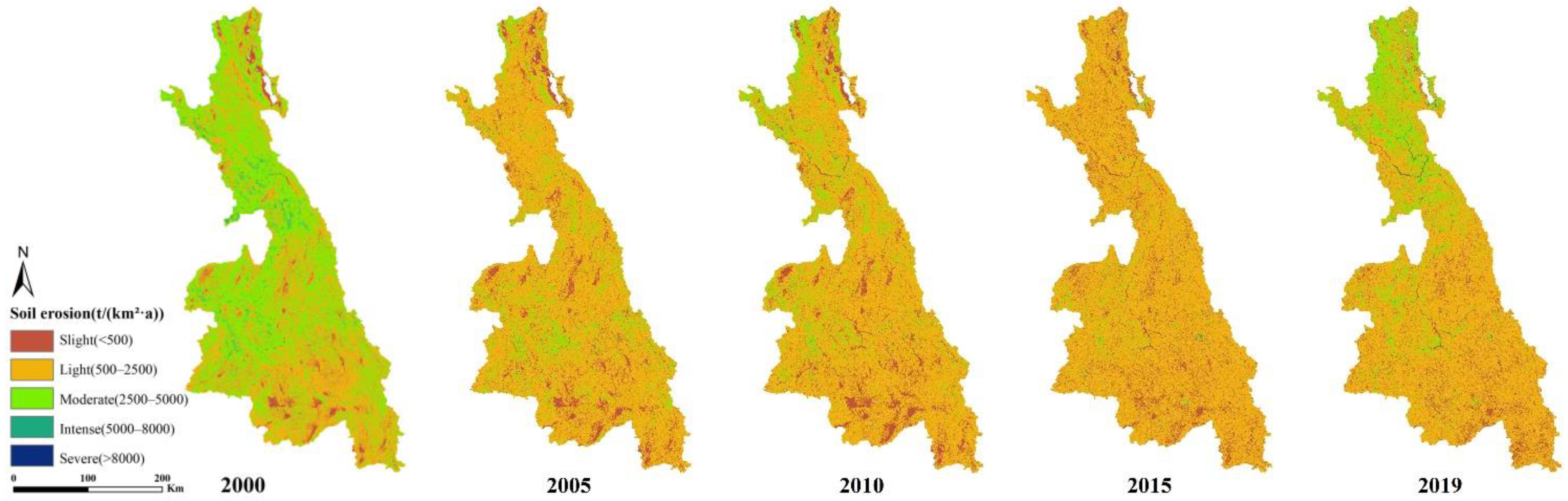
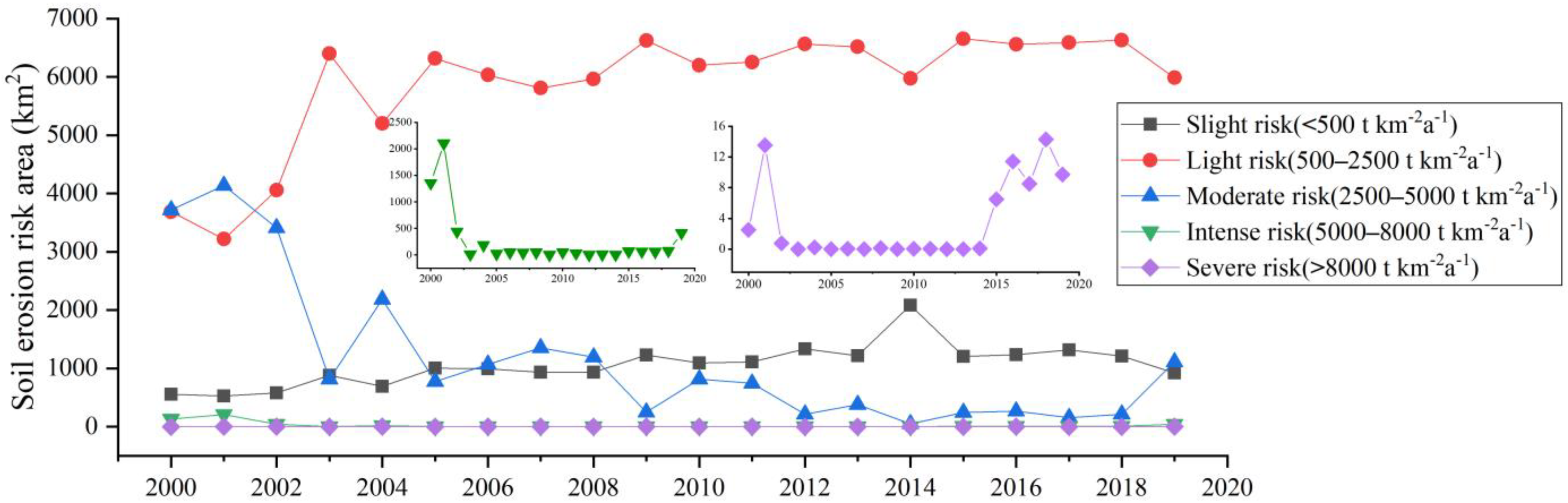
3.1. Spatial Temporal Evolution Characteristics of Soil Erosion

In this study, the RUSLE model was used to calculate the soil erosion moduli of the ML-LRB during 2000–2019 (Figure 2). According to statistics, during the nearly two-decade period of 2000–2019, the average soil erosion modulus in the ML-LRB was 1.52 × 10³ t/(km²·a). The present study showed very little difference compared with the results of many scholars on the average soil erosion modulus in the LRB, and the overall spatial distribution trend was generally consistent [8,18,30,46]. The average soil erosion modulus in 2000 was 2.39 × 10³ t/(km²·a), and the average soil erosion modulus in 2005 was 1.49 × 10³ t/(km²·a), a decrease of about 38% compared with 2000. The average soil erosion modulus in 2010 was 1.47 × 10³ t/(km²·a), with no significant change compared with 2005. The average soil erosion modulus in 2015 was 1.13 × 10³ t/(km²·a), another decrease of about 22% compared with 2010. The average soil erosion modulus in 2019 was 1.51 × 10³ t/(km²·a), an increase of about 14% compared to 2015. The research shows that the annual average soil erosion modulus for the ML-LRB decreased in fluctuation during 2000–2014, but it increased from 2015 onwards. In accordance with the common soil erosion risk criteria in China [9], this study classified soil erosion risk levels and plotted the area changes for each erosion risk during 2000–2019 (Figure 3). The areas of soil erosion in the ML-LRB during that decade were mainly of light risk. There was a sharp increase in the light-risk erosion area in the ML-LRB in 2003, reaching a maximum of 63,989.46 km² (77% of the total basin area), but there was little change during the following years. During 2000–2019, the moderate-risk erosion area in the ML-LRB decreased sharply in 2003, with a minimum of 8162.22 km² (representing 10% of the total basin area), but it has stabilized since 2005. The slight-risk erosion area in the ML-LRB increased slowly since 2000 and reached a maximum of 20,859.83 km² in 2014 (representing 25% of the total basin area). The intense- and severe-risk erosion area had a sharp decrease starting in 2001 and stabilized after 2005, but there was a year-to-year increase from 2015 onwards. As shown by the temporal changes of soil erosion in the ML-LRB during 2000–2019, soil erosion during 2000–2010 was characterized by uneven spatial distribution and significant spatial heterogeneity, but after 2010, this heterogeneity gradually weakened within the ML-LRB. Although the soil erosion intensity in the ML-LRB gradually decreased, there was an increase in the slight- and light-risk erosion areas and a decrease in the moderate-risk erosion area. However, since 2015, there was an increase in the moderate- and intense-risk erosion areas in Lincang City in the central part of the ML-LRB and Dali City in the north.

To better understand the spatiotemporal distribution of soil erosion in the ML-LRB, Quantum GIS (QGIS) and the Soil and Water Assessment Tool models were introduced to divide the Middle and Lower reaches of the Lancang River Subbasins (ML-LRS) based on landform and main drainage distribution [47], thereby obtaining a total of 10 subbasins (S1–S10). S1–S4 are in the Middle reach of the Lancang River Subbasins (M-LRS), and S5–S10 are in the Lower reach of the Lancang River Subbasins (L-LRS). Additionally, according to the soil erosion risk criteria, the average soil erosion modulus for the ML-LRB was divided to obtain the spatiotemporal distribution characteristics of erosion risk by subbasin (Figure 4). Thus, in 2000, the ML-LRB subbasins exhibited a gradual decrease in average soil erosion from north to south. S2–S4, S6 and S7 had a moderate erosion risk, whereas other subbasins were mostly within the range of light-risk erosion. The average soil erosion moduli for subbasins S1, S5 and S10 were higher than those for S8 and S9. In 2005, there was a gradual increase in average soil erosion from outside to inside in the ML-LRS. S1–S10 were all within the light risk erosion range, and S2, S5, S6 and S7 had higher average soil erosion modulus than the other subbasins. Unlike 2000, there were two levels of erosion risk reduction in S3 and S4 and one-level reduction in all the other subbasins in 2005. In 2010, there was a gradual decrease in average soil erosion from north to south in the ML-LRS. S2 was in the moderate-risk erosion range, S8 was close to the slight-risk erosion range and all the other subbasins were in the light-risk erosion range. Within the same level, M-LRB were higher than those in the L-LRB, and all had a one-level increase in erosion risk compared to the M-LRS in 2005. The erosion risks of S5, S6 and S8 were reduced by one level in 2010 compared to 2005, while the other subbasins had no significant change. In 2015, there was no significant difference in the spatial distribution of average soil erosion in the ML-LRS. S1–S10 were in the light risk erosion range, whereas S8 and S9 were close to the slight-risk erosion. A comparison of M-LCB, S2, S7 and S9 in 2015 to 2010 revealed that there was a one-level reduction in erosion risk, whereas the other subbasins had no significant change. In 2019, there was a gradual decrease in average soil erosion from north to south in the subbasins and large differences in spatial distribution. There was an above-moderate erosion risk in the M-LRB and a below-slight erosion risk in the L-LRB. Compared with 2015, M-LRB had an increase of one or two levels in 2019. According to this research, during 2000–2019, there was a yearly decrease from north to south in all the ML-LRS. To further define the relationship between soil erosion changes in the ML-LRB and ML-LRS during 2000–2019, this paper plotted the results of changes in the average soil erosion modulus for both reaches over those two decades (Figure 5). Accordingly, ML-LRS had a soil erosion modulus averaging 635.34–2992.23 t/(km²·a), which were mostly below the light-to-moderate risk cutoff. During the same period, there was a yearly decrease in risk in each subbasin, but the pattern of change in the L-LRS more closely matched that of the study area as a whole. During 2000–2019, the improvement in soil erosion in the ML-LRB followed a trend consistent with the research of Wang et al. [48], who previously identified such an improved trend in soil erosion in China since 2000.

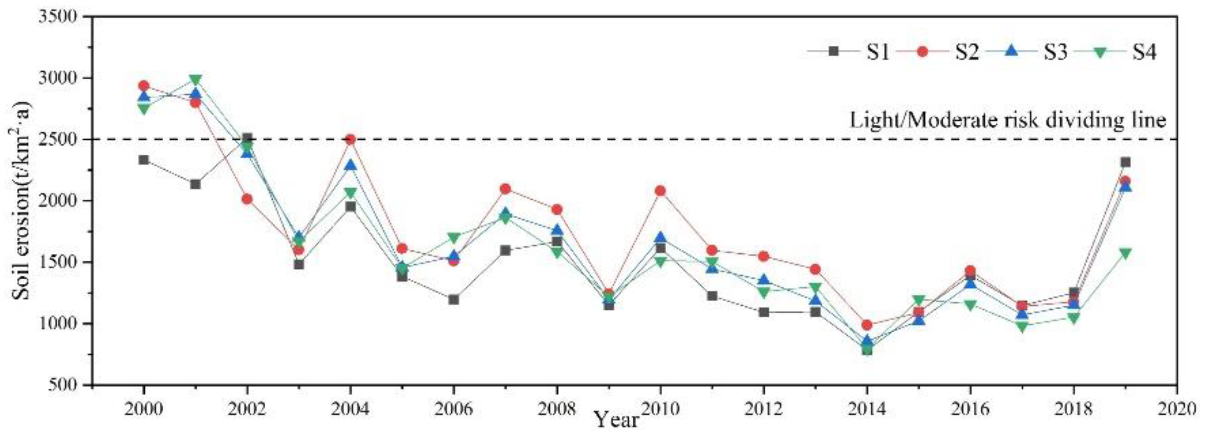
3.2. Trends Analysis in Soil Erosion

Based on the Mann–Kendall modeling, this study performed trend tests to determine the average soil erosion modulus and soil erosion risk areas in the ML-LRB and ML-LRS during 2000–2019 [49]. (

Table 3. Mann–Kendall model results of the average soil erosion modulus and erosion risk area in the ML-LRB and ML-LRS, during 2000–2019.

Mann–Kendall Test	Test Z	p Value	Significance
Soil erosion	−4.19	2.85 × 10−5	**
Slight-risk area	3.54	4.06 × 10−4	**
Light-risk area	3.15	1.65 × 10−3	**
Moderate-risk area	−3.60	3.17 × 10−4	**
Intense-risk area	−0.49	0.63	NA
Severe-risk area	0.98	0.33	NA
Water area	−0.43	0.67	NA
S1	−2.37	0.02	*
S2	−3.15	1.65 × 10−3	**
S3	−3.60	3.15 × 10−4	**
S4	−4.12	3.78 × 10−5	**
S5	−4.57	4.77 × 10−6	**
S6	−4.19	2.85 × 10−5	**
S7	−4.38	1.19 × 10−5	**
S8	−3.67	2.46 × 10−4	**
S9	−4.06	5.00 × 10−5	**
S10	−4.12	3.78 × 10−5	**

Negative Z value indicates a decrease, and a positive Z value indicates an increase. * Statistically significant trends at the 5% significance level. ** Statistically significant trends at the 1% significance level. NA indicates insignificance.

). The trend-test value (Z < 0) for the average soil erosion modulus across the ML-LRB, implying a gradual decrease in the average soil erosion modulus during the two decades, was studied; the significant test value (p < 0.05) indicated a significant decrease. The trend-test value (Z > 0) for the ML-LRB at slight, light and severe erosion risk suggested an overall increase. The significant test value (p < 0.05) for both slight and light erosion risk areas indicated a significant increase, whereas the significant test value (p > 0.05) for severe erosion risk areas indicated an insignificant increase. The trend-test value (Z < 0) for areas with a moderate and intense erosion risk suggested an overall decrease in the areas with a moderate and intense erosion risk in the ML-LRB. The significant test value (p < 0.05) for these areas also revealed a significant decrease. According to the results of the soil erosion modulus tests for the ML-LRS (Z < 0 and p < 0.05), there was a significant decrease. The trend-test showed an increase in areas with a slight and light erosion risk and a decrease in areas with a moderate and intense erosion risk in the ML-LRB, indicating that the decrease in the average soil erosion modulus for the ML-LRB and ML-LRS was mainly attributable to a decline in the area with a moderate and intense erosion risk.

To further derive the spatial-variation characteristics of soil erosion and its influencing factors in the ML-LRB, the Sen’s slope estimation was used together with Mann–Kendall trend model to analyze the spatial-temporal trend changes of soil erosion, rainfall, NDVI and land use for the study area during 2000–2019 (Figure 6). The research found that the spatial distribution of soil erosion trend changes in the ML-LRB from 2000 to 2019 was mainly dominated by a significant decreasing and decreasing variation; the area occupied is 4.57 × 10⁴ km and 2.41 × 10⁴ km, accounting for about 55.30% and 29.16% of the whole study area, respectively. This was followed by an area with increasing soil erosion and an area with significantly increasing soil erosion, which accounted for about 6.89% and 5.01% of the ML-LRB, respectively, located mainly in Dali City and Xishuangbanna. Thus, in the ML-LRB, the areas with decreasing soil erosion were much larger than those with increasing soil erosion, but there was a concentrated increasing in soil erosion in Dali City and Xishuangbanna. The spatial distribution of the decreasing trend in soil erosion areas is positively correlated with the spatial distribution of the decreasing trend of rainfall and land use areas, and negatively correlated with the increasing trend of NDVI area (Figure 6b–d). The results of Sen’s Slope estimation coupled with Mann–Kendall trend model indicate that soil erosion decreases with decreasing rainfall and land use area, and increasing NDVI.

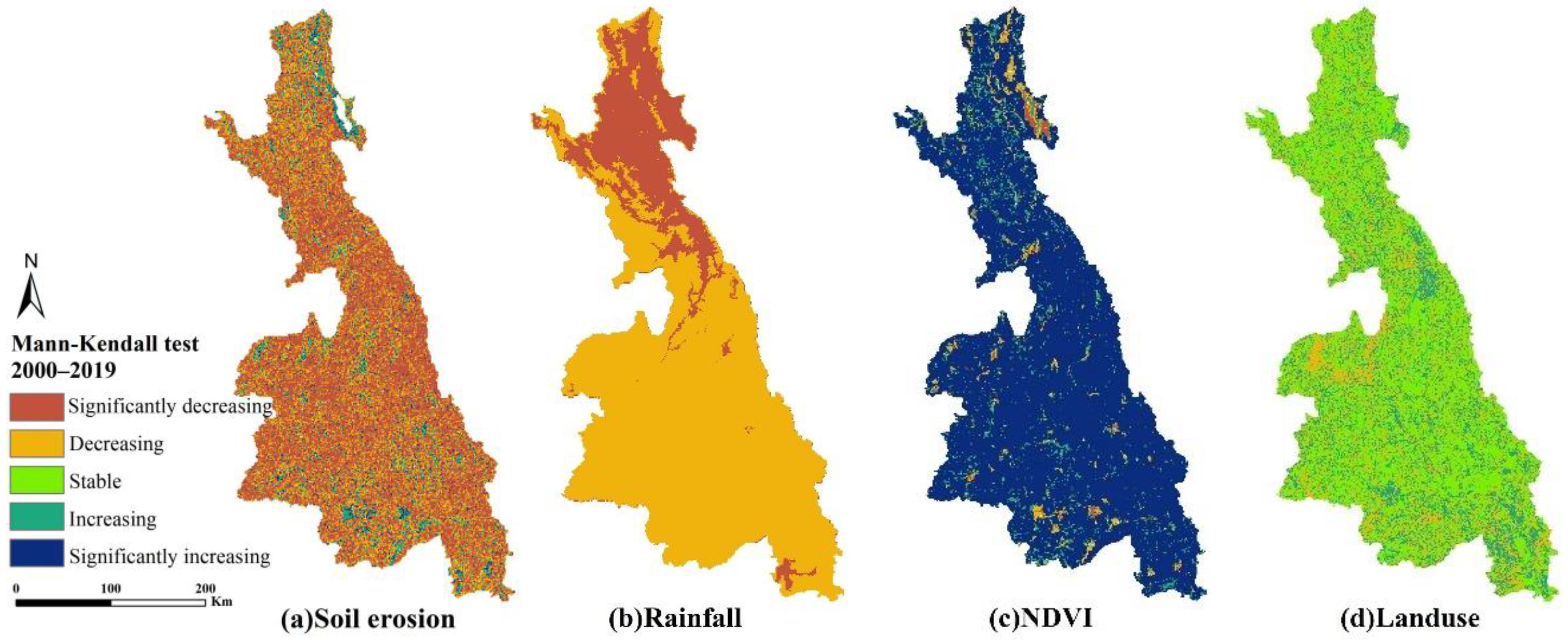
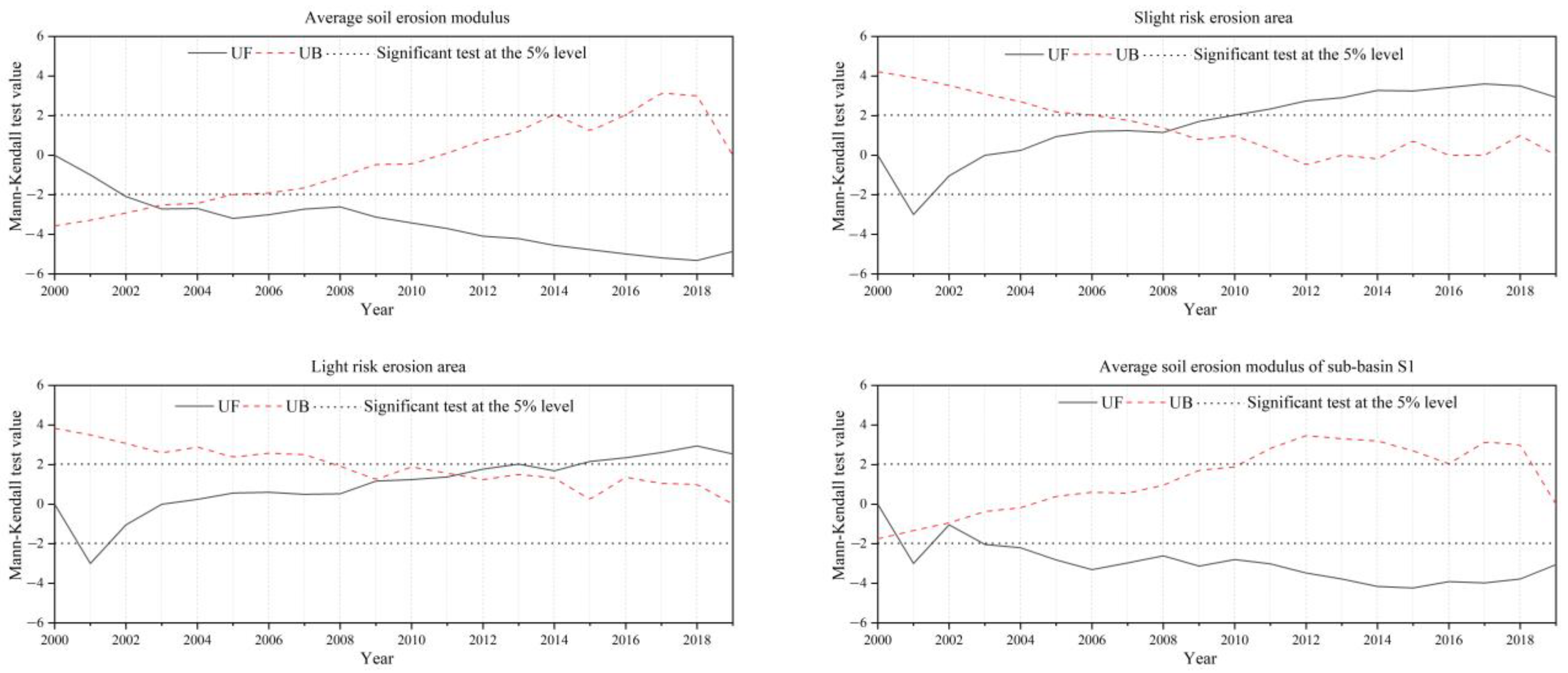
3.3. Mutation Tests in Soil Erosion

The mutation test of average soil erosion modulus and erosion risk area in the ML-LRB and ML-LRS based on Mann–Kendall model was performed, with a significance level set at α = 0.05 (i.e., U0.05 = ±1.96) (Figure 7) [15,50,51]. The results of the mutation test for the average soil erosion modulus in the study area during 2000–2019 show that no mutation occurred in the average soil erosion modulus for the ML-LRB. The results of the mutation test for the average soil erosion modulus in the ML-LRS show that there was a mutation in the average soil erosion modulus in S1 in 2002. The test results for the slight erosion risk area show that that there was a mutation in 2009. The test results for the moderate erosion risk areas in ML-LRB show that UF and UB intersected in 2002, but the intersection fell outside the critical line, suggesting that there was no mutation in the moderate erosion risk areas. According to the above results, S1 (in Dali City) recorded great changes in the soil erosion modulus in 2002, mainly linked to moderate risk erosion, and in 2009, the area of light erosion risk across the ML-LRB experienced significant change.

4. Discussion

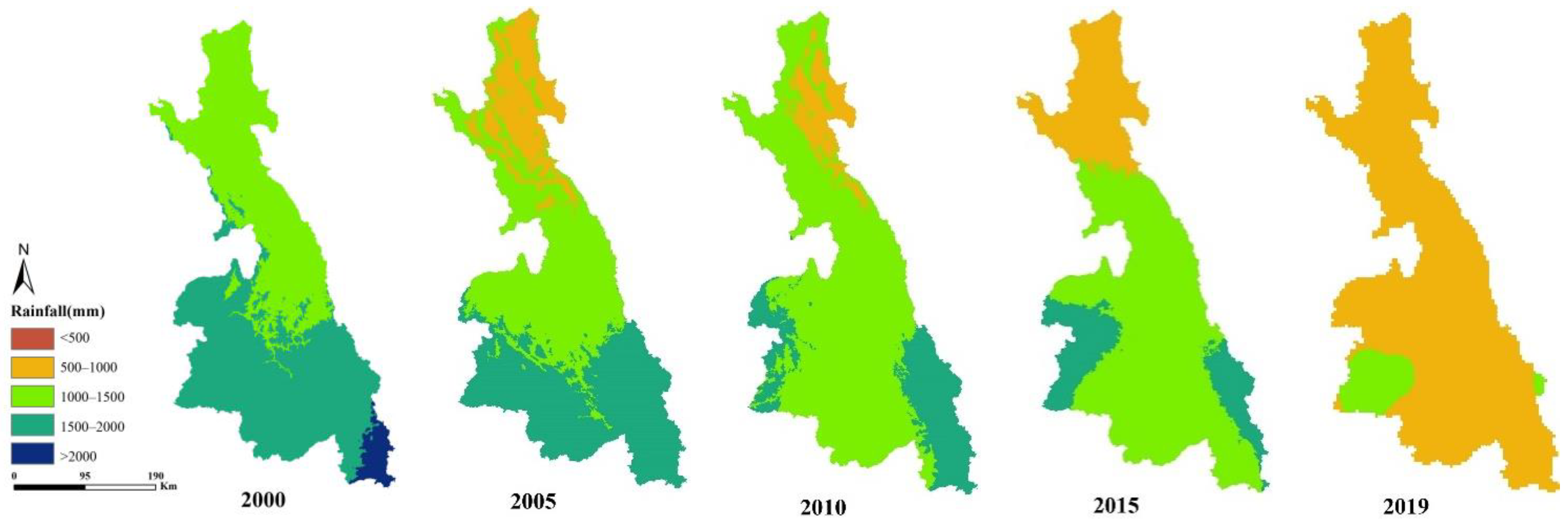
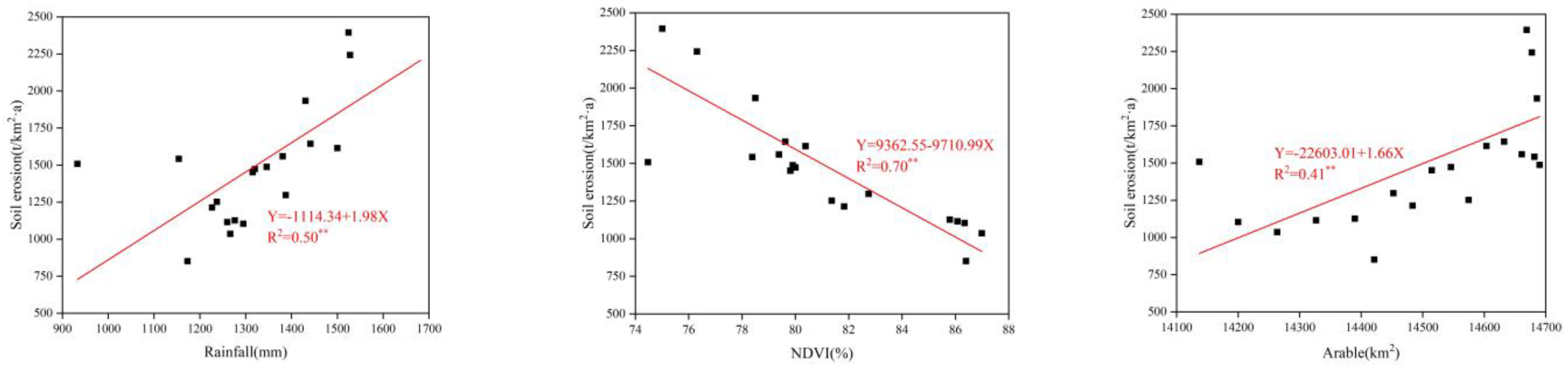
4.1. Main Mechanisms Controlling Changes in Soil Erosion

To further examine the main control mechanism of soil erosion changes, this paper used the Mann–Kendall model to conduct a trend analysis of rainfall, NDVI and land use in the ML-LRB during 2000–2019 (

Table 4. Mann–Kendall model results of rainfall, NDVI and land use in the ML-LCB.

Mann–Kendall Test	Test Z	p Value	Significance
Rainfall	−2.95	3.25 × 10−3	**
NDVI	4.12	3.78 × 10−5	**
Arable Land	−5.1586	2.49 × 10−7	**
Forest Land	2.5631	0.01	*
Grassland	−4.5098	6.49 × 10−6	**
Water Area	3.0963	1.96 × 10−3	**
Urban construction Land	6.132	8.68 × 10−10	**
Unused Land	1.3176	0.19	NA

Negative Z value indicates a decrease, and a positive Z value indicates an increase. * Statistically significant trends at the 5% significance level. ** Statistically significant trends at the 1% significance level. NA indicates insignificance.

). The results of the trend test (Z > 0, p < 0.01) of the NDVI and forest areas indicate a significant increase; the results of the trend test (Z < 0, p < 0.01) of the rainfall, arable and grassland areas show a significant decrease; and the results of the trend test (Z > 0, p < 0.01) of the watershed and urban land areas reveal an overall significant increase.

To further explore the effects of rainfall, NDVI and land use on soil erosion in the ML-LRB, this study plotted the spatiotemporal distributions of rainfall and NDVI in the area during 2000–2019 (Figure 8 and Figure 9). From Figure 8, it can be observed that the rainfall in the ML-LRB was lower in the Upper reaches and higher in the Lower reaches. Since 2005, starting from Dali City in the north, a change occurred: rainfall decreased from north to south, and the annual rainfall in the entire study area did not exceed 1500 mm by 2019. The trend of decreasing rainfall from north to south is coincident with the erosion trend of the soil. There was a gradual increase in NDVI in the study area from upstream to downstream, with the vegetation coverage being basically above 60% (Figure 9). During 2000–2015, the NDVI in the ML-LRB increased each year, with the proportion of the area covered by vegetation (greater than 80%) in the study area increasing from 25.61% in 2000 to 85.23% in 2015, but falling to 40.40% in 2019. The trend of increasing NDVI from north to south improved soil erosion. Using Moderate Resolution Imaging Spectroradiometer (MODIS) images from 2000 to 2015 and local daily climate data since 1976, WeiOuyang’s [27] study found that the spatial variation of NDVI is more sensitive to elevation, temperature and rainfall. Temperature was the main factor influencing LRB grasslands and forest dynamics. Vegetation–climate interactions are more sensitive below a 3000 m elevation. Under the future dry and warm climatic conditions, NDVI in higher elevation, upstream areas may increase soil erosion and decrease streamflow. NDVI in the Lower reaches will improve and be capable of adapting to the associated climatic impacts. Due to the large amount of water and biomass in the watershed, higher temperatures will speed up the decomposition of forest foliar litter. Temperature was not addressed in this study, and in terms of rainfall, the significant decrease in NDVI in 2019 may be due to reduced rainfall. The above study found that the dramatic increase in NDVI in the northern part of the LRB in 2019 was the predominant element for the increase in soil erosion in 2019 in the northern part of the region.

Based on the inflow and outflow characteristics shown on a Sankey diagram, this paper examined the relationship between soil erosion risk area and land use area changes in the ML-LRB during 2000–2010 and 2010–2019 (Figure 10a). The highest proportion of the ML-LRB was the forest, succeeded by arable and grassland areas, while urban land, water and unused land comprised the lowest proportion. During 2000–2010, there were no significant changes in land use in the ML-LRB, but during 2010–2019, there was a significant change in land use across the study area: ~38.34% of the arable land changed to Forest, while ~14.39% changed to grassland; ~10.01% of the forest changed to arable, while ~9.11% changed to grassland; and ~15.01% of the grassland changed to arable, while ~40.58% changed to forest. The remaining parts of the ML-LRB basically experienced no change in land use type. Light- to moderate-erosion risks were most common in the ML-LRB, succeeded by slight-, less-intense and severe-erosion risks (Figure 10b). During 2000–2010, the soil erosion risk areas changed greatly: ~28.21% of the slight changed to light, while ~0.91% changed to moderate; ~15.58% of the light changed to slight, while ~1.71% changed to moderate and ~3.81% of the moderate changed to slight, while ~78.42% changed to light. There was no significant change in the rest of the erosion risk areas. During 2010–2019, the soil erosion risk areas also had great changes: ~63.99% of the slight changed to light, while ~6.61% changed to moderate; ~9.54% of the light changed to slight, while ~11.76% changed to moderate and ~2.81% of the moderate changed to slight, while ~55.71% changed to light. This study interpreted Sankey diagrams for 2000–2010 and 2010–2019 as indicating that soil erosion was only slightly affected by land use change in the earlier period, but greatly affected by it in the later period.

From the above results, this paper established a regression model linking soil erosion, rainfall, NDVI and arable area in the ML-LRB (Figure 11). Accordingly, the variation of soil erosion showed a significant positive correlation with rainfall and arable areas [52], and established a significantly negative correlation with NDVI. The research of Borrelli et al. [53] also showed that larger arable areas might aggravate global soil erosion. Despite the large number of hills and mountains in the ML-LRB, there was a yearly increase in areas with vegetation cover (greater than 80%) [53,54]. Through further research, Burneo et al. [55] found that, even with steep slopes and high annual rainfall, protected areas of evergreen vegetation are at only slight soil erosion risk. The above results imply that soil erosion before 2010 in the ML-LRB was influenced mainly by rainfall and NDVI, succeeded by arable areas, whereas soil erosion after 2010 was influenced mainly by arable areas and NDVI, succeeded by rainfall.

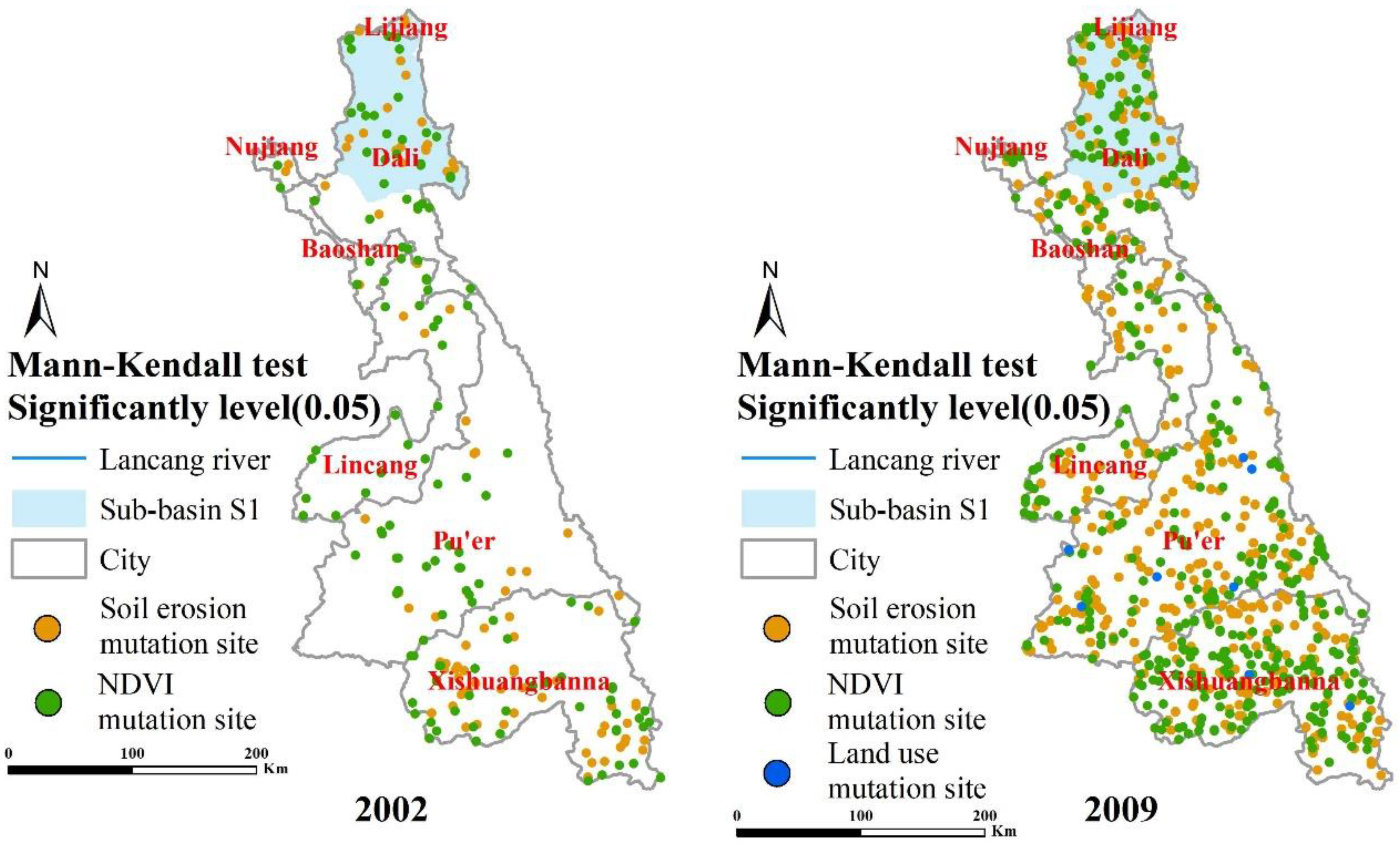
4.2. Main Reasons for Controlling Mutations in Soil Erosion

Previous studies on mutations have focused on a long time-series dataset. This study used the Mann–Kendall mutation model to investigate whether the mean or median of the long time-series dataset mutated over years of variation. Although this is a scientific method for the nonparametric testing of individual time-series datasets for mutated years, mutations in time are not necessarily the result of mutations in space. Spatially, there are both decreased and increased mutations, which, when the mean, median or cumulative values are taken into consideration, may result in a decrease or increase in the area of mutation because of mutual cancellation. If the Mann–Kendall model is introduced to test long time-series remote-sensing datasets that have great spatial heterogeneity, it is difficult to determine whether the creation or disappearance of temporal mutations is the result of spatial mutations or the data-standardization process of taking the mean, median or cumulative values of remote-sensing datasets that have great spatial heterogeneity. There are mutations of the average soil erosion modulus in 2002 in S1 as well as in the light erosion risk areas in 2009 in the ML-LRB (Section 3.3). Hence, to confirm the reasons for the spatiotemporal mutations, this paper used the Mann–Kendall mutation model to calculate the UF and UB statistical values corresponding to soil erosion, rainfall, NDVI and land use in 2002 and in 2009. Then, we plotted the mutational site changes in the ML-LRB during those two years based on the principle of UF/UB intersection, and with mutational sites meeting the significance level (0.05) test. As is evident from the results, only soil erosion and NDVI had spatial mutational sites in 2002 and 2009 (Figure 12). Soil erosion mutation sites in the ML-LRB in 2002 were mainly in Dali City in the Upper reach and in Xishuangbanna in the Lower reach, but only S1 in the northeastern part of Dali City had mutations, and S8 and S9 in Xishuangbanna had no mutations. This may be because of several causes: The soil erosion area in S1 generally decreased, and in spite of a small amount of increasing soil erosion area in the northeastern part of the subbasin, there was no significant mutual offset in the data standardization; the areas of increased soil erosion in Xishuangbanna were mostly mixed with areas of reduced soil erosion, resulting in no mutation in the average soil erosion modulus for S8 and S9; and the mutational sites of soil erosion and NDVI in S1 intersected and overlapped several times, indicating that the temporal mutation in 2002 primarily resulted from the greater extent of areas with a decreasing soil erosion modulus in S1 compared to those with an increasing modulus, whereas the spatial mutation of soil erosion was mainly a result of the mutation of NDVI. According to the trend analysis of the ML-LRB, the areas with a decreasing trend were much larger than those with an increasing trend (Figure 6). The mutational sites of soil erosion and NDVI in 2009 were mixed and evenly distributed throughout the basin, and there were intersections with land use as well. This suggests that the temporal mutation of light erosion risk areas in the ML-LRB in 2009 was mainly because of the change of moderate and intense to light erosion risk areas, and the spatial mutation was mainly influenced by NDVI and potentially also related to land use.

5. Conclusions

By coupling Sen’s slope estimation and the Mann–Kendall model, this paper studied the trends of soil erosion and its influencing factors in the ML-LRB, thus further identifying the mutation areas of soil erosion. According to the results, the average soil erosion modulus in the ML-LRB was 1.52 × 10³ t/(km²·a) during 2000–2019, which was at a light erosion risk level. Soil erosion had an uneven spatial distribution and significant spatial heterogeneity in the ML-LRB during 2000–2010 and exhibited a substantial reduction after 2010. Despite the benign reduction trend of the soil erosion intensity in the ML-LRB, attention should be placed on the increase in moderate and intense erosion risk areas in Lincang and Dali City since 2015. On the basis of landforms and the main drainage distribution in the ML-LRB, this paper divided the study area into ten subbasins (S1–S10) using hydrological calculations. The research shows that, during 2000–2019, there was a yearly decrease in the average soil erosion modulus of the subbasins from north to south, and the areas with decreased soil erosion were much larger than those with increased soil erosion. The results of the linear regression model show that soil erosion was significantly positively correlated with rainfall and arable area and significantly negatively correlated with NDVI. According to the test results using the Mann–Kendall model, the temporal mutation in 2002 primarily resulted from the much greater extent of the areas with decreasing soil erosion modulus in S1 than those with increasing soil erosion modulus, and the spatial mutation of soil erosion was mainly a result of the mutation of NDVI. The temporal mutation of light erosion risk areas in the ML-LRB in 2009 was mainly due to the change of moderate and intense erosion risk areas to light, and the spatial mutation was mainly influenced by NDVI and potentially also related to land use.

References

1. Poesen, J. Soil erosion in the Anthropocene: Research needs. Earth Surf. Processes Landf. J. Br. Geomorphol. Res. Group 2018, 43, 64–84. [Google Scholar] [CrossRef]
2. Wuepper, D.; Borrelli, P.; Finger, R. Countries and the global rate of soil erosion. Nat. Sustain. 2020, 3, 51–55. [Google Scholar] [CrossRef]
3. Liu, H.; Zhang, G.; Zhang, P.; Zhu, S. Spatial Distribution and Temporal Trends of Rainfall Erosivity in Three Gorges Reservoir Area of China. Math. Probl. Eng. 2020, 2020, 5302679. [Google Scholar] [CrossRef]
4. Guo, B.; Yang, G.; Zhang, F.; Han, F.; Liu, C. Dynamic monitoring of soil erosion in the upper Minjiang catchment using an improved soil loss equation based on remote sensing and geographic information system. Land Degrad. Dev. 2018, 29, 521–533. [Google Scholar] [CrossRef]
5. Olorunfemi, I.E.; Komolafe, A.A.; Fasinmirin, J.T. A GIS-based assessment of the potential soil erosion and flood hazard zones in Ekiti State, Southwestern Nigeria using integrated RUSLE and HAND models. Catena 2020, 194, 104725. [Google Scholar] [CrossRef]
6. Alewell, C.; Meusburger, K.; Brodbeck, M.; Bänninger, D. Methods to describe and predict soil erosion in mountain regions. Landsc. Urban Plan. 2008, 88, 46–53. [Google Scholar] [CrossRef]
7. Wang, J.; Sun, G.; Shi, F.; Lu, T.; Wang, Q.; Wu, Y.; Wu, N.; Oli, K.P. Runoff and soil loss in a typical subtropical evergreen forest stricken by the Wenchuan earthquake: Their relationships with rainfall, slope inclination, and vegetation cover. J. Soil Water Conserv. 2014, 69, 65–74. [Google Scholar] [CrossRef]
8. Chuenchum, P.; Xu, M.; Tang, W. Predicted trends of soil erosion and sediment yield from future land use and climate change scenarios in the Lancang–Mekong River by using the modified RUSLE model. Int. Soil Water Conserv. Res. 2020, 8, 213–227. [Google Scholar] [CrossRef]
9. Duan, X.; Bai, Z.; Rong, L.; Li, Y.; Li, J.; Wang, W. Investigation method for regional soil erosion based on the Chinese Soil Loss Equation and high-resolution spatial data: Case study on the mountainous Yunnan Province, China. Catena 2020, 184, 104237. [Google Scholar] [CrossRef]
10. Vaezi, A.R.; Abbasi, M.; Keesstra, S.; Cerdà, A. Assessment of soil particle erodibility and sediment trapping using check dams in small semi-arid catchments. Catena 2017, 157, 227–240. [Google Scholar] [CrossRef] [Green Version]
11. Krasa, J.; Dostal, T.; Jachymova, B.; Bauer, M.; Devaty, J. Soil erosion as a source of sediment and phosphorus in rivers and reservoirs—Watershed analyses using WaTEM/SEDEM. Environ. Res. 2019, 171, 470–483. [Google Scholar] [CrossRef] [PubMed]
12. Mushi, C.A.; Ndomba, P.M.; Trigg, M.A.; Tshimanga, R.M.; Mtalo, F. Assessment of basin-scale soil erosion within the Congo River Basin: A review. Catena 2019, 178, 64–76. [Google Scholar] [CrossRef]
13. Vijith, H.; Dodge-Wan, D. Spatial and statistical trend characteristics of rainfall erosivity (R) in upper catchment of Baram River, Borneo. Environ. Monit. Assess. 2019, 191, 494. [Google Scholar] [CrossRef] [PubMed]
14. Ali, R.; Kuriqi, A.; Abubaker, S.; Kisi, O. Long-Term Trends and Seasonality Detection of the Observed Flow in Yangtze River Using Mann-Kendall and Sen’s Innovative Trend Method. Water 2019, 11, 1855. [Google Scholar] [CrossRef] [Green Version]
15. Xu, M.; Kang, S.; Wu, H.; Yuan, X. Detection of spatio-temporal variability of air temperature and precipitation based on long-term meteorological station observations over Tianshan Mountains, Central Asia. Atmos. Res. 2018, 203, 141–163. [Google Scholar] [CrossRef]
16. Ganasri, B.P.; Ramesh, H. Assessment of soil erosion by RUSLE model using remote sensing and GIS—A case study of Nethravathi Basin. Geosci. Front. 2015, 7, 953–967. [Google Scholar] [CrossRef] [Green Version]
17. Fu, B.; Yu, L.; Lue, Y.; He, C.; Yuan, Z.; Wu, B. Assessing the soil erosion control service of ecosystems change in the Loess Plateau of China. Ecol. Complex. 2011, 8, 284–293. [Google Scholar] [CrossRef]
18. Suif, Z.; Fleifle, A.; Yoshimura, C.; Saavedra, O. Spatio-temporal patterns of soil erosion and suspended sediment dynamics in the Mekong River Basin. Sci. Total Environ. 2016, 568, 933–945. [Google Scholar] [CrossRef] [Green Version]
19. Alewell, C.; Borrelli, P.; Meusburger, K.; Panagos, P. Using the USLE: Chances, challenges and limitations of soil erosion modelling—ScienceDirect. Int. Soil Water Conserv. Res. 2019, 7, 203–225. [Google Scholar] [CrossRef]
20. Phinzi, K.; Ngetar, N.S. The assessment of water-borne erosion at catchment level using GIS-based RUSLE and remote sensing: A review. Int. Soil Water Conserv. Res. 2019, 7, 27–46. [Google Scholar] [CrossRef]
21. Sinha, T.; Cherkauer, K.A. Time Series Analysis of Soil Freeze and Thaw Processes in Indiana. J. Hydrometeorol. 2008, 9, 936–950. [Google Scholar] [CrossRef] [Green Version]
22. Gocic, M.; Trajkovic, S. Analysis of changes in meteorological variables using Mann-Kendall and Sen’s slope estimator statistical tests in Serbia. Glob. Planet. Chang. 2013, 100, 172–182. [Google Scholar] [CrossRef]
23. Da Silva, R.M.; Santos, C.A.; Moreira, M.; Corte-Real, J.; Silva, V.C.; Medeiros, I.C. Rainfall and river flow trends using Mann-Kendall and Sen’s slope estimator statistical tests in the Cobres River basin. Nat. Hazards 2015, 77, 1205–1221. [Google Scholar] [CrossRef]
24. Shi, W.; Yu, X.; Liao, W.; Wang, Y.; Jia, B. Spatial and temporal variability of daily precipitation concentration in the Lancang River basin, China. J. Hydrol. 2013, 495, 197–207. [Google Scholar] [CrossRef]
25. Zhai, H.J.; Hu, B.; Luo, X.Y.; Qiu, L.; Tang, W.J.; Jiang, M. Spatial and temporal changes in runoff and sediment loads of the Lancang River over the last 50 years. Agric. Water Manag. 2016, 174, 74–81. [Google Scholar] [CrossRef]
26. Li, J.; Dong, S.; Yang, Z.; Peng, M.; Liu, S.; Li, X. Effects of cascade hydropower dams on the structure and distribution of riparian and upland vegetation along the middle-lower Lancang-Mekong River. For. Ecol. Manag. 2012, 284, 251–259. [Google Scholar] [CrossRef]
27. Ouyang, W.; Wan, X.; Xu, Y.; Wang, X.; Lin, C. Vertical difference of climate change impacts on vegetation at temporal-spatial scales in the upper stream of the Mekong River Basin. Sci. Total Environ. 2019, 701, 134782. [Google Scholar] [CrossRef]
28. Liu, S.; An, N.; Yang, Y.; Dong, Y.; WANG, C. Effects of different land-use types on soil organic carbon and its prediction in the mountain-ous areas in the middle reaches of Lancang River. Chin. J. Appl. Ecol. 2015, 26, 981–988. [Google Scholar]
29. Lu, Q.; Gai, A.; Liu, Y.; Ma, Z.; Pan, T. The change of land use and cover and its impacts o landscape pattern in Lancang River Basin based GIS. J. Gansu Agric. Univ. 2018, 53, 113–119. [Google Scholar]
30. Pavisorn, C.; Xu, M.; Tang, W. Estimation of Soil Erosion and Sediment Yield in the Lancang–Mekong River Using the Modified Revised Universal Soil Loss Equation and GIS Techniques. Water 2019, 12, 135. [Google Scholar] [CrossRef] [Green Version]
31. Brown, L.C.; Foster, G.R. Storm Erosivity Using Idealized Intensity Distributions. Trans. ASAE 1987, 30, 0379–0386. [Google Scholar] [CrossRef]
32. Wischmeier, W.H.; Smith, D.D. Predicting rainfall erosion losses: A guide to conservation planning. In Agriculture Handbook; No. 537; USDA: Washington, DC, USA, 1978. [Google Scholar]
33. Guidelines for demarcating ecological conservation red lines. In Environmental Work Information Selection; Ministry of Ecology and Environment of the People’s Republic of China: Beijing, China, 2017; pp. 19–23.
34. Thomas, J.; Sabu Joseph, K.P.; Thrivikramji. Estimation of soil erosion in a rain shadow river basin in the southern Western Ghats, India using RUSLE and transport limited sediment delivery function. Int. Soil Water Conserv. Res. 2017, 6, 111–122. [Google Scholar] [CrossRef]
35. Van der Knijff, J.M.; Jones, R.J.; Montanarella, L. Soil Erosion Risk Assessment in Europe; European Commission: Brussels, Belgium, 2000; pp. 7–23. [Google Scholar]
36. Zhu, Q.; Guo, J.; Guo, X.; Han, Y.; Chen, L.; Luo, H. Research on Influencing Factors of Soil Erosion Based on Random Forest Algorithm—A Case Study in Upper Reaches of Ganjiang River Basin. Bull. Soil Water Conserv. 2020, 40, 59–68. [Google Scholar]
37. Yang, D.; Kanae, S.; Oki, T.; Koike, T.; Musiake, K. Global potential soil erosion with reference to land use and climate changes. Hydrol. Processes 2003, 17, 2913–2928. [Google Scholar] [CrossRef]
38. Chen, H.; Oguchi, T.; Pan, W.U. Assessment for soil loss by using a scheme of alterative sub-models based on the RUSLE in a Karst Basin of Southwest China. J. Integr. Agric. 2017, 16, 377–388. [Google Scholar] [CrossRef] [Green Version]
39. Li, S.; Zhu, Z.; Lv, L.; Guo, S. Soil erosion characteristics of the Prince Edward River basin based on the RUSLE model. Water Resour. Power 2020, 38, 5. [Google Scholar]
40. Zhou, Q.; Shi, X.; Fu, Y.; He, J.; Li, Q. Analysis of Soil Erosion Characteristics of the Upstream of the Fenhe River Based on RUSLE. Yellow River 2020, 42, 6. [Google Scholar]
41. Mann, H.B. Nonparametric test against trend. Econometrica 1945, 13, 245–259. [Google Scholar] [CrossRef]
42. Kendall, M.G. Rank Correlation Methods. Br. J. Psychol. 1990, 25, 86–91. [Google Scholar] [CrossRef]
43. Atta-ur-Rahman; Dawood, M. Spatio-statistical analysis of temperature fluctuation using Mann–Kendall and Sen’s slope approach. Clim. Dyn. 2017, 48, 783–797. [Google Scholar] [CrossRef]
44. Kisi, O.; Ay, M. Comparison of Mann-Kendall and innovative trend method for water quality parameters of the Kizilirmak River, Turkey. J. Hydrol. 2014, 513, 362–375. [Google Scholar] [CrossRef]
45. Sen, K.P. Estimates of the Regression Coefficient Based on Kendall’s Tau. Publ. Am. Stat. Assoc. 1968, 63, 1379–1389. [Google Scholar] [CrossRef]
46. Wu, F.; Zhu, Y.; Xu, D.; Shi, J.; Jiang, Y. Assessment of soil erosion and prioritization for treatment at the catchment level in the Mekong basin. Acta Ecol. Sin. 2019, 39, 4761–4772. [Google Scholar]
47. Molina-Navarro, E.; Nielsen, A.; Trolle, D. A QGIS plugin to tailor SWAT watershed delineations to lake and reservoir waterbodies. Environ. Model. Softw. 2018, 108, 67–71. [Google Scholar] [CrossRef]
48. Wang, X.; Zhao, X.; Zhang, Z.; Yi, L.; Zuo, L. Assessment of soil erosion change and its relationships with land use/cover change in China from the end of the 1980s to 2010. Catena 2016, 137, 256–268. [Google Scholar] [CrossRef]
49. Mueller, E.N.; Pfister, A. Increasing occurrence of high-intensity rainstorm events relevant for the generation of soil erosion in a temperate lowland region in Central Europe. J. Hydrol. 2011, 411, 266–278. [Google Scholar] [CrossRef]
50. Zhao, Y.; Pu, Y.; Lin, H.; Tang, R. Examining Soil Erosion Responses to Grassland Conversation Policy in Three-River Headwaters, China. Sustainability 2021, 13, 2702. [Google Scholar] [CrossRef]
51. Stefanidis, S.; Chrysoula, C. Response of soil erosion in a mountainous catchment to temperature and precipitation trends. Carpathian J. Earth Environ. Sci. 2017, 12, 35–39. [Google Scholar]
52. Zhou, J.; Fu, B.; Gao, G.; Lü, Y.; Liu, Y.; Lü, N.; Wang, S. Effects of precipitation and restoration vegetation on soil erosion in a semi-arid environment in the Loess Plateau, China. Catena 2016, 137, 1–11. [Google Scholar] [CrossRef]
53. Borrelli, P.; Robinson, D.A.; Fleischer, L.R.; Lugato, E.; Ballabio, C.; Alewell, C.; Meusburger, K.; Modugno, S.; Schütt, B.; Ferro, V. An assessment of the global impact of 21st century land use change on soil erosion. Nat. Commun. 2017, 8, 2013. [Google Scholar] [CrossRef] [PubMed] [Green Version]
54. Sun, W.; Shao, Q.; Liu, J.; Zhai, J. Assessing the effects of land use and topography on soil erosion on the Loess Plateau in China. Catena 2014, 121, 151–163. [Google Scholar] [CrossRef]
55. Burneo, J.I.; Fries, A.; Mejia, D.; Cerda, A.; Ochoa, P.A.; Ruiz-Sinoga, J.D. Effects of climate, land cover and topography on soil erosion risk in a semiarid basin of the Andes. Catena Interdiscip. J. Soil Sci. Hydrol. Geomorphol. Focusing Geoecology Landsc. Evol. 2016, 140, 31–42. [Google Scholar]
Figure 1. Research area.
Sustainability 14 05169 g001
Figure 2. Spatial and temporal distribution of soil erosion risk in the ML-LRB, during 2000–2019.
Sustainability 14 05169 g002
Figure 3. Spatial and temporal distribution characteristics of soil erosion in the ML-LRB and ML-LRS.
Sustainability 14 05169 g003
Figure 4. Spatial and temporal distribution characteristics of soil erosion in the ML-LRS, during 2000–2019. Note: S1–S4 are the M-LRS and S5–S10 are the L-LRS.
Sustainability 14 05169 g004
Figure 5. Changes of the annual average soil erosion modulus in the ML-LRB and ML-LRS, during 2000–2019. Note: The dotted line represents the light to moderate erosion risk division (2500 t/km2·a).
Sustainability 14 05169 g005aSustainability 14 05169 g005b
Figure 6. Spatial-temporal trend changes of soil erosion, rainfall, NDVI and land use for the ML-LRB during 2000–2019.
Sustainability 14 05169 g006
Figure 7. Mann–Kendall mutation criterion curve of soil erosion and erosion risk area in the ML-LCR and ML-LRS from 2000 to 2019. Note: At the significance level of α = 0.05, if UF and UB intersected at the confidence zone, the year corresponding to that point was the year of abrupt change in soil erosion change.
Sustainability 14 05169 g007
Figure 8. Spatial distribution of rainfall in the ML-LCB during 2000–2019.
Sustainability 14 05169 g008
Figure 9. Spatial distribution of NDVI in the ML-LCB during 2000–2019.
Sustainability 14 05169 g009
Figure 10. Land use and soil erosion risk area transfer Sankey map. (a) 2000–2010 and 2010–2019 land use area; (b) 2000–2010 and 2010–2019 soil erosion risk area.
Sustainability 14 05169 g010
Figure 11. Soil erosion in relation to rainfall, NDVI and arable area on the ML-LRB during 2000–2019; ** Significant correlation at the 1% level.
Sustainability 14 05169 g011
Figure 12. Regional mutation site distribution of soil erosion, NDVI and land use in the ML-LCB.
Sustainability 14 05169 g012