
The Impact of Economic Growth, Industrial Transition, and Energy Intensity on Carbon Dioxide Emissions in China


Abstract
:1. Introduction
2. Literature Review and Related Hypotheses
2.1. Literature Review
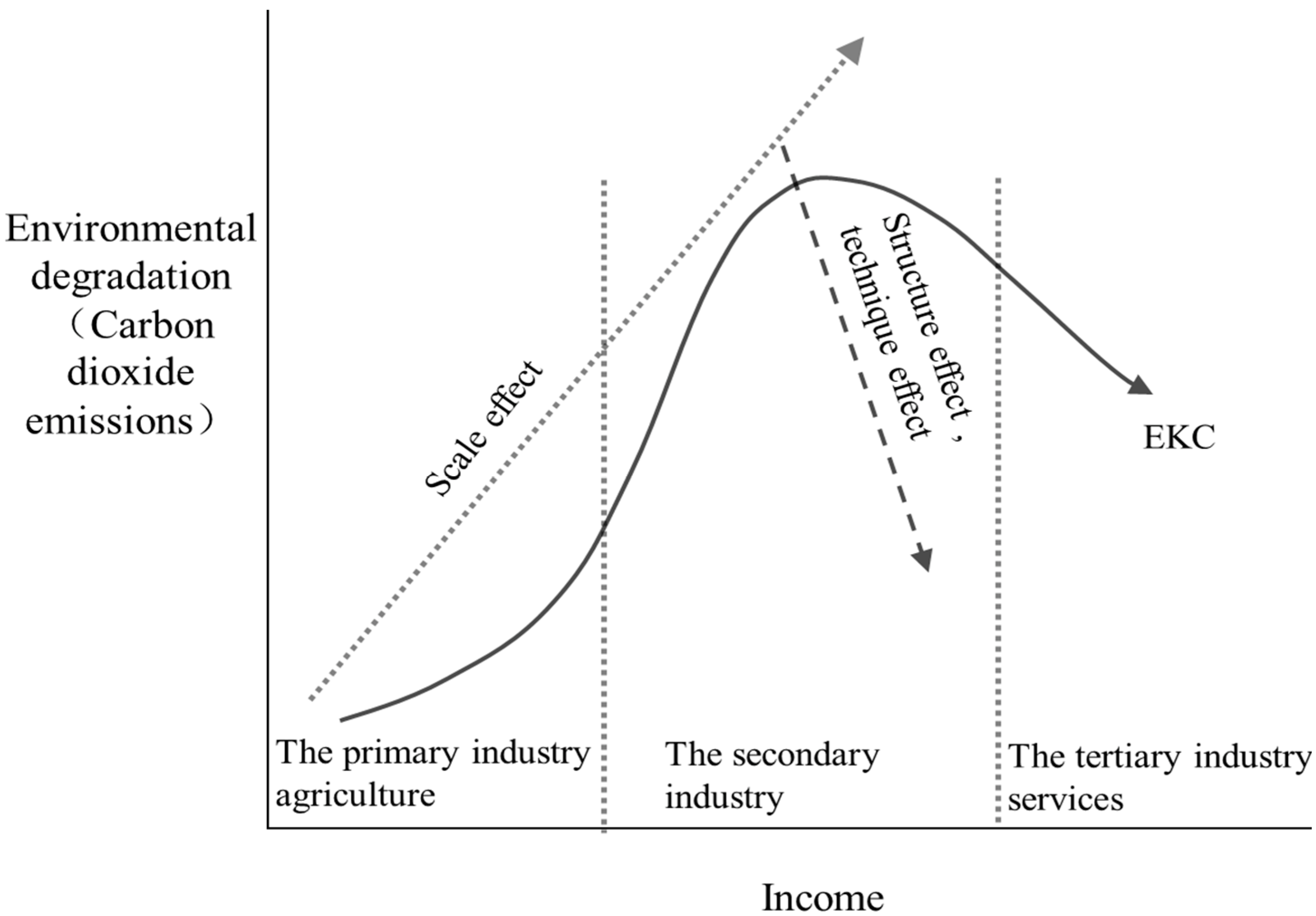
2.1.1. Scale Effect, Structure Effect, and Technique Effect
2.1.2. Energy Intensity
2.2. Research Hypotheses
3. Data and Method
3.1. Data
- Economic growth () and its quadratic term. GDP was treated as the proxy variable of economic growth and the scale effect to eliminate the influence of price factors, and GDP was converted to the constant price in 1980. These terms were included in the independent variables to examine the EKC hypothesis [19,43,45].
- Industry transition (). The proportion of added value of secondary industry in GDP calculated at current prices was not only chosen for the proxy variable of the industrial transition, but also taken as the proxy variable of the structure effect.
- Energy intensity (). Since energy intensity is a measure of energy efficiency [46,47,48], which can reflect the level of technology, this paper selects energy intensity as the proxy variable of technique effect. Furthermore, whether energy intensity has a significant reduction effect or rebound effect on CO2 emissions was explored.
3.2. Model Estimation
3.3. Econometric Methodology
4. Results
4.1. Unit Root Test
4.2. Bounds Test
4.3. Econometric Model Results
4.3.1. ARDL Short-Run Results
4.3.2. ARDL Long-Run Results
4.3.3. Residual Diagnostics
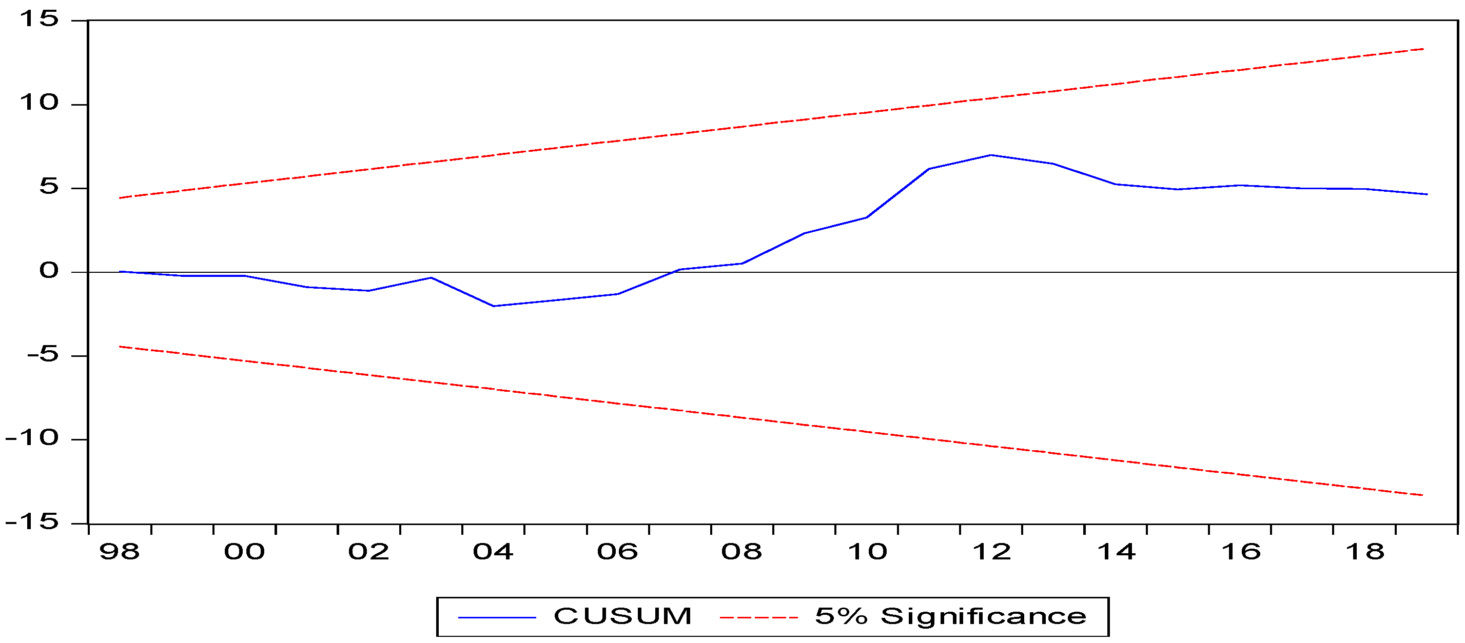
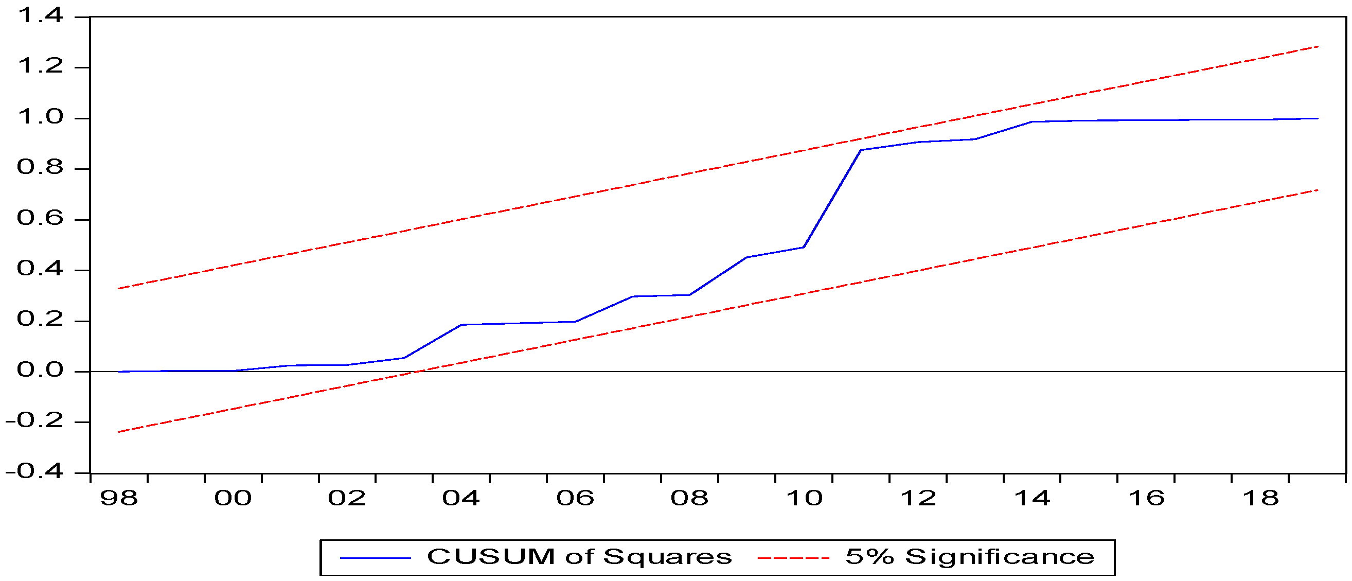
4.3.4. Model Stability Diagnosis
5. Conclusions and Policy Implications
Author Contributions
Funding
Institutional Review Board Statement
Informed Consent Statement
Data Availability Statement
Acknowledgments
Conflicts of Interest
References
- Zhang, S.; Chen, W. Assessing the energy transition in China towards carbon neutrality with a probabilistic framework. Nat. Commun. 2022, 13, 87. [Google Scholar] [CrossRef] [PubMed]
- United Nations Environment Programme (UNEP). Emissions Gap Report 2020. Available online: https://www.unenvironment.org/zh-hans/emissions-gap-report-2020 (accessed on 16 January 2022).
- UNFCCC. Decision 1/CP.21, Adoption of the Paris Agreement, Advance Unedited Version. 2015. Available online: http://www.researchgate.net/publication/311746574_Decision_1CP21_Adoption_of_the_Paris_Agreement_Advance_unedited_version (accessed on 15 December 2021).
- Masson-Delmotte, V.; Zhai, P.; Pörtner, H.; Roberts, D.; Skea, J.; Shukla, P.R.; Pirani, A.; Moufouma-Okia, W.; Péan, C.; Pidcock, R.; et al. Global Warming of 1.5 °C; An IPCC Special Report on the Impacts of Global Warming of 1.5 °C above Pre-Industrial Levels and Related Global Greenhouse Gas Emission Pathways, in the Context of Strengthening the global Response to the Threat of Climate Change, Sustainable Development, and Efforts to Eradicate Poverty; IPCC: Geneva, Switzerland, 2018; Available online: https://iefworld.org/node/947 (accessed on 16 December 2021).
- Team, P.; Carbon, P.; Neutrality, C. Analysis of a Peaked Carbon Emission Pathway in China Toward Carbon Neutrality. Engineering 2021, 7, 1673–1677. [Google Scholar] [CrossRef]
- The Energy and Climate Intelligence Unit. Net zero Emissions Race. 2021. Available online: https://eciu.net/netzerotrack (accessed on 16 January 2022).
- Zhang, S.; Chen, W. China’s energy transition pathway in a carbon neutral vision. Engineering 2021, in press. [CrossRef]
- Wang, H.; Lu, X.; Deng, Y.; Sun, Y.; Nielsen, C.P.; Liu, Y.; Zhu, G.; Bu, M.; Bi, J.; McElroy, M.B. China’s CO2 peak before 2030 implied from characteristics and growth of cities. Nat. Sustain. 2019, 2, 748–754. [Google Scholar] [CrossRef]
- Xi, J.P. Statement at the General Debate of the 75th Session of the United Nations General Assembly. In Gazette of the State Council of the People’s Republic of China; The State Council of the People’s Republic of China: Beijing, China, 2020; Volume 28, pp. 5–7. Available online: http://en.people.cn/n3/2020/0923/c90000-9763272.html (accessed on 16 January 2022).
- Wang, W.; Yang, Z.; Zhang, B.; Lu, Y.; Shi, Y. The optimization degree of provincial industrial ecosystem and EKC of China—based on the grey correlation analysis. In Proceedings of the IEEE International Conference on Grey Systems and Intelligent Services (GSIS), Leicester, UK, 18–20 August 2015; pp. 179–186. [Google Scholar] [CrossRef]
- Kaika, D.; Zervas, E. The Environmental Kuznets Curve (EKC) theory-Part A: Concept, causes and the CO2 emissions case. Energy Policy 2013, 62, 1392–1402. [Google Scholar] [CrossRef]
- Debone, D.; Leite, V.P.; Georges, S.; Khouri, E. Urban Climate Modelling approach for carbon emissions, energy consumption and economic growth: A systematic review. Urban Clim. 2021, 37, 100849. [Google Scholar] [CrossRef]
- Li, W.; Yang, G.; Li, X.; Sun, T.; Wang, J. Cluster analysis of the relationship between carbon dioxide emissions and economic growth. J. Clean. Prod. 2019, 225, 459–471. [Google Scholar] [CrossRef]
- Dong, B.; Ma, X.; Zhang, Z.; Zhang, H.; Chen, R.; Song, Y.; Shen, M.; Xiang, R. Carbon emissions, the industrial structure and economic growth: Evidence from heterogeneous industries in China*. Environ. Pollut. 2020, 262, 114322. [Google Scholar] [CrossRef]
- Saint, S.; Adewale, A.; Olasehinde-williams, G.; Udom, M. Science of the Total Environment The role of electricity consumption, globalization and economic growth in carbon dioxide emissions and its implications for environmental sustainability targets. Sci. Total Environ. 2020, 708, 134653. [Google Scholar] [CrossRef]
- Sheng, P.; Li, J.; Zhai, M.; Majeed, M.U. Economic growth efficiency and carbon reduction efficiency in China: Coupling or decoupling. Energy Rep. 2021, 7, 289–299. [Google Scholar] [CrossRef]
- Sarfraz, M.; Ivascu, L.; Cioca, L.-I. Environmental Regulations and CO2 Mitigation for Sustainability: Panel Data Analysis (PMG, CCEMG) for BRICS Nations. Sustainability 2022, 14, 72. [Google Scholar] [CrossRef]
- Lu, Z.N.; Chen, H.; Hao, Y.; Wang, J.; Song, X.; Mok, T.M. The dynamic relationship between environmental pollution, economic development and public health: Evidence from China. J. Clean. Prod. 2017, 166, 134–147. [Google Scholar] [CrossRef]
- Grossman, G.; Krueger, A. Environmental Impacts of a North American Free Trade Agreement; Working Paper; National Bureau of Economic Research: Cambridge, MA, USA, 1991; p. 3194. Available online: http://refhub.elsevier.com/S0959-6526(20)33416-8/sref29 (accessed on 15 December 2021).
- Grossman, G.W.; Krueger, A.B. Economic Growth and Environment. Q. J. Econ. 1995, 110, 357–378. Available online: https://academic.oup.com/qje/article-abstract/110/2/353/1826336?redirectedFrom=fulltext (accessed on 15 December 2021). [CrossRef] [Green Version]
- Panayotou, T. Empirical Test and Policy Analysis of Environmental Degradation at Different Stages of Economic Development; World Employment Research Programme, Working Paper WP; International Labour Office: Geneva, Switzerland, 1993; p. 238. Available online: http://refhub.elsevier.com/S0959-6526(20)33416-8/sref62 (accessed on 15 December 2021).
- Kaika, D.; Zervas, E. The environmental Kuznets curve (EKC) theory. Part B: Critical issues. Energy Policy 2013, 62, 1403–1411. [Google Scholar] [CrossRef]
- Selden, T.; Song, D. Environmental quality and development: Is there a Kuznets curve for air pollution emissions? J. Environ. Econ. Manag. 1994, 27, 147–162. [Google Scholar] [CrossRef]
- Dinda, S.; Coondoo, D.; Pal, M. Air quality and economic growth: An empirical study. Ecol. Econ. 2000, 34, 409–423. [Google Scholar] [CrossRef]
- Panayotou, T. Economic Growth and the Environment. In Economic Survey of Europe; Chapter 2; UNECE: Geneva, Switzerland, 2003; Volume 2. [Google Scholar]
- Dinda, S. Environmental Kuznets Curve hypothesis: A survey. Ecol. Econ. 2004, 49, 431–455. [Google Scholar] [CrossRef] [Green Version]
- Du, L.; Wei, C.; Cai, S. Economic development and carbon dioxide emissions in China: Provincial panel data analysis. China Econ. Rev. 2012, 23, 371–384. [Google Scholar] [CrossRef]
- De Bruyn, S.M.; Van Den Bergh, J.C.J.M.; Opschoor, J.B. Economic growth and emissions: Reconsidering the empirical basis of environmental Kuznets curves. Ecol. Econ. 1998, 25, 161–175. [Google Scholar] [CrossRef]
- Robalino-López, A.; Mena-Nieto, A.; García-Ramos, J.E. System dynamics modeling for renewable energy and CO2 emissions: A case study of Ecuador. Energy Sustain. Dev. 2014, 20, 11–20. [Google Scholar] [CrossRef] [Green Version]
- Shafiei, S.; Salim, R.A. Non-renewable and renewable energy consumption and CO2 emissions in OECD countries: A comparative analysis. Energy Policy 2014, 66, 547–556. [Google Scholar] [CrossRef] [Green Version]
- López-Menéndez, A.J.; Pérez, R.; Moreno, B. Environmental costs and renewable energy: Re-visiting the Environmental Kuznets Curve. J. Environ. Manag. 2014, 145, 368–373. [Google Scholar] [CrossRef] [PubMed]
- Saidi, K.; Hammami, S. The impact of energy consumption and CO2 emissions on economic growth: Fresh evidence from dynamic simultaneous-equations models. Sustain. Cities Soc. 2015, 14, 178–186. [Google Scholar] [CrossRef]
- Tol, R.S.J.; Pacala, S.W.; Socolow, R.H. Understanding Long-Term Energy Use and Carbon Dioxide Emissions in the USA. J. Policy Model. 2009, 31, 425–445. [Google Scholar] [CrossRef] [Green Version]
- Begum, R.A.; Sohag, K.; Abdullah, S.M.S.; Jaafar, M. CO2 emissions, energy consumption, economic and population growth in Malaysia. Renew. Sustain. Energy Rev. 2015, 41, 594–601. [Google Scholar] [CrossRef]
- Yang, Z.; Zhao, Y. Energy consumption, carbon emissions, and economic growth in India: Evidence from directed acyclic graphs. Econ. Model. 2014, 38, 533–540. [Google Scholar] [CrossRef]
- Kasman, A.; Duman, Y.S. CO2 emissions, economic growth, energy consumption, trade and urbanization in new EU member and candidate countries: A panel data analysis. Econ. Model. 2015, 44, 97–103. [Google Scholar] [CrossRef]
- Shahbaz, M.; Solarin, S.A.; Sbia, R.; Bibi, S. Does energy intensity contribute to CO2 emissions? A trivariate analysis in selected African countries. Ecol. Indic. 2015, 50, 215–224. [Google Scholar] [CrossRef] [Green Version]
- Stern, D.I. Energy and economic growth. In Encyclopedia of Energy; Cleveland, C.J., Ed.; Academic Press: San Diego, CA, USA, 2004; pp. 35–51. [Google Scholar] [CrossRef]
- Tiwari, A.K. The asymmetric Granger-causality analysis between energy consumption and income in the United States. Renew. Sustain. Energy Rev. 2014, 36, 362–369. [Google Scholar] [CrossRef]
- Greening, L.A.; Greene, D.L.; Difiglio, C. Energy efficiency and consumption—The rebound effect—A survey. Energy Policy 2000, 28, 389–401. [Google Scholar] [CrossRef]
- Hanley, N.; McGregor, P.G.; Swales, J.K.; Turner, K. Do increases in energy efficiency improve environmental quality and sustainability? Ecol. Econ. 2009, 68, 692–709. [Google Scholar] [CrossRef]
- Dimitropoulos, J. Energy productivity improvements and the rebound effect: An overview of the state of knowledge. Energy Policy 2007, 35, 6354–6363. [Google Scholar] [CrossRef]
- Lin, H.; Wang, X.; Bao, G.; Xiao, H. Heterogeneous Spatial Effects of FDI on CO2 Emissions in China. Earth’s Future 2022, 10, e2021EF002331. [Google Scholar] [CrossRef]
- Lin, B.; Zhu, J. Energy and carbon intensity in China during the urbanization and industrialization process: A panel VAR approach. J. Clean. Prod. 2020, 168, 780–790. [Google Scholar] [CrossRef]
- Fang, K.; Li, C.; Tang, Y.; He, J.; Song, J. China’s pathways to peak carbon emissions: New insights from various industrial sectors. Appl. Energy 2022, 306, 118039. [Google Scholar] [CrossRef]
- Dietz, T.; Rosa, E.A. Effects of Population and Affluence on CO2 Emissions. Proc. Natl. Acad. Sci. USA 1997, 94, 175–179. [Google Scholar] [CrossRef] [PubMed] [Green Version]
- Shafique, M.; Azam, A.; Rafiq, M.; Luo, X. Investigating the nexus among transport, economic growth and environmental degradation: Evidence from panel ARDL approach. Trans. Policy 2021, 109, 61–71. [Google Scholar] [CrossRef]
- Zhang, Z.; Guo, S. What Factors Affect the RMB Carry Trade Return for Sustainability? An Empirical Analysis by Using an ARDL Model. Sustainability 2021, 13, 13533. [Google Scholar] [CrossRef]
- Alam, K.M.; Baig, S.; Li, X.; Ghanem, O.; Hanif, S. Causality between transportation infrastructure and economic development in Pakistan: An ARDL analysis. Res. Trans. Econ. 2020, 88, 100974. [Google Scholar] [CrossRef]
- Abbasi, K.R.; Shahbaz, M.; Jiao, Z.; Tufail, M. How energy consumption, industrial growth, urbanization, and CO2 emissions affect economic growth in Pakistan? A novel dynamic ARDL simulations approach. Energy 2021, 221, 119793. [Google Scholar] [CrossRef]
- Pesaran, M.H.; Shin, Y. An autoregressive distributed-lag modelling approach to cointegration analysis. Econ. Soc. Monogr. 1998, 31, 371–413. Available online: http://refhub.elsevier.com/S0301-4207(19)30921-3/optcvJLWnzrJv (accessed on 15 December 2021).
- Abubakr, R.; Hooi, H.; Shahbaz, M. Are too many natural resources to blame for the shape of the Environmental Kuznets Curve in resource-based economies? Resour. Policy 2020, 68, 101694. [Google Scholar] [CrossRef]
- William, H. Greene. Economic Analysis; Prentice Hall: Hoboken, NJ, USA, 2003. [Google Scholar]
- Uddin, G.S.; Shahbaz, M.; Arouri, M.; Teulon, F. Financial development and poverty reduction nexus: A cointegration and causality analysis in Bangladesh. Econ. Model. 2014, 36, 405–412. [Google Scholar] [CrossRef] [Green Version]
- Zaman, Q.; Wang, Z.; Zaman, S.; Rasool, S.F. Investigating the nexus between education expenditure, female employers, renewable energy consumption and CO2 emission: Evidence from China. J. Clean. Prod. 2021, 312, 127824. [Google Scholar] [CrossRef]
- Tanizaki, H. Asymptotically exact confidence intervals of CUSUM and CUSUMSQ tests: A numerical derivation using simulation technique. Commun. Stat. Simulat. Comput. 1995, 24, 1019–1036. Available online: http://refhub.elsevier.com/S0959-6526(21)02042-4/sref63 (accessed on 15 December 2021). [CrossRef] [Green Version]


| Variable Name | Code | Unit | Implication |
|---|---|---|---|
| CO2 emissions | CARBON | Ton | Environmental degradation |
| GDP | GDP | 1980 constant price yuan | Economic growth, scale effect |
| Proportion of the added value of the secondary industry | INDUSTRY | % | Industrial transition, structure effect |
| Energy intensity | ENERGY | Kilograms of standard coal per unit added value | Technique effect |
| Variables | Augmented Dicey-Fuller | Phillips-Perron |
|---|---|---|
| (ADF) | (PP) | |
| Level | Test-Statistic Value | |
| 2.2704 | 4.2438 | |
| −1.7452 | −1.7367 | |
| −0.2391 | −2.3307 | |
| −0.7178 | −1.1312 | |
| −2.8692 *** | −5.0581 *** | |
| First Difference | Test-Statistic Value | |
| −3.1115 ** | −3.2551 ** | |
| −3.8251 *** | −3.3237 ** | |
| −3.9623 *** | −3.4891 ** | |
| −3.9028 *** | −3.8744 *** | |
| −1.9751 ** | −1.7283 * |
| Test Statistics | Value | |
|---|---|---|
| F-statistic | 4.968918 | |
| Critical Value Bounds | ||
| Significance | Lower Bound | Upper Bound |
| 10% | 2.20 | 3.09 |
| 5% | 2.56 | 3.49 |
| 2.50% | 2.88 | 3.87 |
| 1% | 3.29 | 4.37 |
| Variable | Coefficient | t-Statistics |
|---|---|---|
| 0.18 | 1.5431 | |
| 0.25 ** | 2.6302 | |
| 10.34 *** | 4.5566 | |
| 5.72 ** | 2.3315 | |
| −0.49 *** | −4.1719 | |
| −0.34 ** | −2.5862 | |
| 0.46 *** | 3.0803 | |
| 1.23 *** | 6.8269 | |
| −0.18 | −0.6518 | |
| −0.70 *** | −3.8473 | |
| −0.60 *** | −6.3749 |
| Variable | Coefficient | t-Statistics |
|---|---|---|
| 2.56 *** | 5.4005 | |
| −0.05 ** | −2.8085 | |
| 0.60 ** | 2.2700 | |
| 1.77 *** | 9.4489 | |
| −13.13 *** | −3.8448 |
| Breusch-Godfrey LM Test | Breusch-Pagan-Godfrey Test | |
|---|---|---|
| F-statistic | 0.3355 | 1.6343 |
| (p-value) | (0.7189) | (0.1466) |
| -statistic | 1.2011 | 18.8629 |
| (p-value) | (0.5485) | (0.1703) |
Publisher’s Note: MDPI stays neutral with regard to jurisdictional claims in published maps and institutional affiliations. |
© 2022 by the authors. Licensee MDPI, Basel, Switzerland. This article is an open access article distributed under the terms and conditions of the Creative Commons Attribution (CC BY) license (https://creativecommons.org/licenses/by/4.0/).
Share and Cite
Yang, Z.; Cai, J.; Lu, Y.; Zhang, B. The Impact of Economic Growth, Industrial Transition, and Energy Intensity on Carbon Dioxide Emissions in China. Sustainability 2022, 14, 4884. https://doi.org/10.3390/su14094884
Yang Z, Cai J, Lu Y, Zhang B. The Impact of Economic Growth, Industrial Transition, and Energy Intensity on Carbon Dioxide Emissions in China. Sustainability. 2022; 14(9):4884. https://doi.org/10.3390/su14094884
Chicago/Turabian StyleYang, Zhoumu, Jingjing Cai, Yun Lu, and Bin Zhang. 2022. "The Impact of Economic Growth, Industrial Transition, and Energy Intensity on Carbon Dioxide Emissions in China" Sustainability 14, no. 9: 4884. https://doi.org/10.3390/su14094884
APA StyleYang, Z., Cai, J., Lu, Y., & Zhang, B. (2022). The Impact of Economic Growth, Industrial Transition, and Energy Intensity on Carbon Dioxide Emissions in China. Sustainability, 14(9), 4884. https://doi.org/10.3390/su14094884