Machine Learning and Deep Learning in Energy Systems: A Review

Abstract

With population increases and a vital need for energy, energy systems play an important and decisive role in all of the sectors of society. To accelerate the process and improve the methods of responding to this increase in energy demand, the use of models and algorithms based on artificial intelligence has become common and mandatory. In the present study, a comprehensive and detailed study has been conducted on the methods and applications of Machine Learning (ML) and Deep Learning (DL), which are the newest and most practical models based on Artificial Intelligence (AI) for use in energy systems. It should be noted that due to the development of DL algorithms, which are usually more accurate and less error, the use of these algorithms increases the ability of the model to solve complex problems in this field. In this article, we have tried to examine DL algorithms that are very powerful in problem solving but have received less attention in other studies, such as RNN, ANFIS, RBN, DBN, WNN, and so on. This research uses knowledge discovery in research databases to understand ML and DL applications in energy systems’ current status and future. Subsequently, the critical areas and research gaps are identified. In addition, this study covers the most common and efficient applications used in this field; optimization, forecasting, fault detection, and other applications of energy systems are investigated. Attempts have also been made to cover most of the algorithms and their evaluation metrics, including not only algorithms that are more important, but also newer ones that have received less attention.

1. Introduction

Today, with the development of human society and its vital need for energy, energy systems play a very important and decisive role in all aspects of society, especially the domestic sector, industry and transportation [1]. In general, among the important and vital issues related to energy systems, is their ability to respond to supply and demand, having optimal performance and minimal environmental impact. Due to the increase in population and the need to supply the demand for energy in order to provide greater welfare and comfort, and also the increasing use of fossil fuels and their destructive environmental effects, special attention should be paid to these issues [2,3].

Use of renewable resources and systems for purposes such as reducing destructive environmental effects, beneficial economic prospects and safe operation, etc. is one of the ways to deal with the aforementioned problems. For optimal and practical use, accurate knowledge of the determining parameters in these systems as well as their important output parameters is required. Because renewable systems are strongly influenced by their environment and surrounding conditions, it is essential that we use methods and models to forecast these changes and contribute to system productivity and energy management. In other words, the need for a tool to understand the relationship between different parameters and make full use of this data is important. For example, in order to know the power generation of a wind system, it is necessary to predict the speed and direction of wind in an area [4,5]. In relation to photovoltaic systems and solar power plants, it is necessary to predict the intensity and direction of solar radiation in an area to estimate the production capacity [6]. Many more are listed in their respective sections. In addition, due to the exponential growth of data production worldwide in the second half of the twentieth century, as well as the huge amount of data generated by intelligent sensors as a result of technological advances, such as the entry of the Internet of Things (IoT) into energy systems, data-driven models are very efficient. Regarding the growth of data production, it is worthwhile to mention that in 2013, it was reported that 4.4 ZB of data was produced, used and exchanged in the world, but this number was about ten times higher in 2019 [7].

In general, based on the study of Zhao et al. [8], models are divided into two categories based on knowledge driven-based and data driven-based in order to predict and facilitate energy systems. Knowledge-based methods are generally developed based on a deep understanding of systems and their mechanisms, so they require a lot of experience and information, and the possibility of error in them is high [9]. However, data driven-based methods, especially those based on artificial intelligence, which is a subset, since they do not require prior knowledge and a detailed analytical model, and can only be used with appropriate data and general knowledge of the system, can be used very well and have received a lot of attention. Today, the problem of lack of data is almost solved, which can lead to more interest and attention in this direction [10]. Therefore, the applications and algorithms of the newest and most practical models based on data and artificial intelligence, which are called machine learning and deep learning, have become very popular and widely used.

In general, in dealing with issues related to artificial intelligence, we encounter two perspectives. If we are looking for a time factor in the face of the data in the problem, the problem should also be examined from the perspective of Time Series (TS), whose application algorithms are known and are given in the relevant section. But if the time dimension does not matter, we only use the main and conventional machine learning algorithms. Generally, the time dimension is very important in predicting critical parameters, and therefore the model should include both conventional and basic machine learning algorithms and time series algorithms to achieve accurate results. Regarding renewable systems, we can say that with the rise of renewable energy, it is becoming increasingly important to represent time-varying input data in energy system optimization studies. Time-series aggregation, which reduces model complexity, has emerged in recent years to address this challenge [11].

As can be seen from Figure 1, the number of ML articles in the field of energy systems has increased significantly in recent years which indicates its importance, high usage, and considerable ability to analyze related issues to energy systems. It is also clear from Figure 1 that the main upward trend in the number of articles in this field is from 2012, which can be attributed to the further development of DL and its widespread use in scientific issues. In addition, in Figure 2, which was obtained with the help of VOSviewer software, we can see the relationship between different fields in energy systems with ML and DL. The larger the diameter of the circles associated with each keyword in the output image from VOSviewer, the more repetitive that keyword is compared to others in the articles. In energy articles in the field of artificial intelligence, the two keywords ‘machine learning’ and ‘deep learning’ are often used more than ‘artificial intelligence’. Since this analysis is based on the keywords in the articles and this software, ‘artificial intelligence’ is smaller in diameter than ‘machine learning’ and ‘deep learning’. VOSviewer is a software tool for constructing and visualizing bibliometric networks.

From reviewing articles and studies in this field, we find that in most cases, the 10 most well-known ML algorithms have been used in certain applications, and in articles in this field, although we see less creativity and innovation. There are many uses for a variety of ML and DL algorithms that need to be addressed. It is suggested that forthcoming studies of other algorithms, such as the Convolutional Neural Network (CNN), Long-Short Term Memory (LSTM), etc. should be initiated and the results should be reported. In connection with the wide applications of DL and ML in this field, more creative studies are expected in various applications that have a more indirect but equally highly important relationship with energy. For example, Turetskyy et al. [13] developed a method for designing the production of a Lithium-ion battery, which is a leading energy storage technology based on ANN. The purpose is to determine the structure and properties of the intermediate product required for the process steps to achieve a certain quality in the final product of the battery cell.

This paper is a review study on the use and applications of algorithms and models of ML and DL on energy systems, due to their efficiency and high importance. This article also tries to cover more methods and models than other review articles in this field. In a separate section, the various applications of this science in relation to energy systems are discussed in a way that has not been studied before. This article is divided into seven sections: Section 2 deals with the main applications and cases in which ML and DL have been used in energy systems and explanations are given regarding the comparison of the performance of the algorithms; Section 3 describes ML and its algorithms, and also their application in the field of energy systems; Section 4 describes DL and its algorithms, and also their application in the field of energy systems; Section 5 describes TS and its algorithms, and also their application in the field of energy systems; Section 6 deals with the parameters and metrics used to evaluate the accuracy and error calculation of algorithms and models; and Section 7 provides general conclusions from this study.

2. The Main Applications of ML and DL in Energy Systems

ML and DL can be used in many areas related to energy systems. In this section, the main, most common, and growing applications of this science in the field of energy systems are pointed out so that those interested in this field can find a better understanding and view of the use of these models.

2.1. Energy Consumption and Demand Forecast

ML- and DL-based forecasting techniques are widely used in the field of energy systems. Some of the applications used for forecasting in this field are power and load demand forecasting, building energy consumption forecasting, electrical load forecasting and so on [14,15,16]. Globally, buildings have a large share of total energy consumption and waste. Therefore, reducing energy consumption in buildings is an effective way to minimize the negative effects of climate change [17]. This is why most studies and research are conducted to predict energy consumption and demand for buildings. According to the forecast time horizon, existing research on building energy forecasting, like other applications, can be generally classified into three categories: short-term (i.e., up to one week ahead), medium-term (i.e., from one week to one year ahead), and long-term forecasts (i.e., more than one year ahead) [18].

Predicting energy demand in buildings is important at many levels, from a single household unit to the country level. Control and optimization of devices’ performance not only helps balance supply and demand through on-site renewable energy sources (as with the case of nearly zero energy buildings) at the household level, but also helps with installation planning and cost reduction in energy systems [19]. It is very important to obtain complete information about the electricity consumption of the residents because it is possible to improve the accuracy of load forecasting and ensure the normal operation of power systems, energy management, and planning [20].

The summary and results of some interesting and new studies in this field are reviewed below.

Amasyali et al. reviewed recent research into predicting the energy consumption of buildings using most ML and DL algorithms. In most previous articles, in relation to the type of buildings studied, the focus has been on commercial and educational buildings; while also to predict energy consumption in terms of time horizon, more work has been conducted on short-term forecasts. The results of this study show that ML-based models show acceptable performance for this purpose, but all models have specific strengths and weaknesses. They have different functions in different situations and it is not the case that one model can be used for different conditions and applications; each model should be used for a specific application that has a better performance. Another result of this review article is that there exists a gap in the literature for some topics, such as long-term forecast of building energy consumption, forecast of residential building energy consumption, and forecast of lighting energy consumption of the building, all of which need more attention [21].

Deb et al. conducted a comprehensive review of nine TS forecasting techniques, including Fuzzy, Case-Based Reasoning (CBR), Support Vector Machine (SVM), Moving Average (MA) & Exponential Smoothing (ES), Neural Networks (NN), Gray, ANN, Hybrid Model (HM) and Autoregressive Integrated Moving Average (ARIMA) for building energy consumption. This paper considers basic qualitative and quantitative comparisons for all nine techniques mentioned. It should be noted that the HM is considered as a technique among the nine techniques presented and further explanation of the various combinations of the HM, while evaluating their performance and novelty, is another goal of this article. One of the important results of this paper is that a combination of TS prediction techniques, such as ANN and ARIMA, can be combined well with optimization techniques such as Genetic Algorithm (GA), Particle Swarm Optimization (PSO), and so on [22].

Walker et al. used some ML algorithms to predict electricity demand on an hourly basis, including Boosted-Tree (BT), Random Forest (RF), SVM, and ANN using data from 47 commercial buildings collected over two years. The results showed that by examining the accuracy and prediction error, the RF model showed better performance for this purpose [23].

Grimaldo et al. combined the k Nearest Neighbor (kNN) algorithm with visual analytics to predict and analyze energy supply and demand. This provides results with acceptable accuracy, allowing the user to analyze different forecasting options and relate them to input parameters to identify consumption and production patterns [24].

Hagh et al. proposed an HM to predict home appliance power consumption and peak customer demand, which includes SVM faster clustering (faster clustering k-medoids) and ANN. This model shows a very desirable accuracy of 99.2%, which makes the experimental results of the proposed model effective using smart meter data [25].

Hafeez et al. proposed an innovative HM for short-term electrical load prediction that includes an information preparation model called Modified Mutual Information (MMI), a DL model called Factored Conditional Restricted Boltzmann Machine (FCRBM), and an optimization model called Genetic Wind-Driven Optimization (GWDO). The results, after comparing this model with models such as Mutual Information (MI)-based ANN, Accurate and Fast Converging (AFC)-based ANN, and LSTM. show better performance in terms of accuracy, average runtime, and convergence rate [26].

Khan et al. proposed a model called Cuckoo Search Neural Network (CSNN) by combining Cuckoo Search (CS) and ANN to improve the accuracy, convergence time, and compatibility for Organization of Petroleum Exporting Countries (OPEC) power consumption forecasting. The results of comparing this model with models such as Accelerated Particle Swarm Optimization Neural Network (APSONN), Genetic Algorithm Neural Network (GANN), and Artificial Bee Colony Neural Network (ABCNN) clearly show that this model is more efficient, more powerful, and more compatible with the latest algorithms [27].

Kazemzadeh et al. suggested an HM for long-term prediction of peak electrical load and total electrical energy demand using three models: ARIMA, ANN, and PSO-Support Vector Regression (SVR). According to the results presented in this study, the HM has the best performance among the four models studied (HM > PSO-SVR > ANN > ARIMA) [28].

Fathi et al. conducted an interesting review study on energy performance prediction of urban buildings by considering the type of buildings, type of energy, and time horizon, which examined almost all widely used algorithms in this field. The results show that the most common algorithms used in published articles for this application are ANN and SVR. It should also be noted that studies have been conducted to predict the energy performance of buildings based on electrical energy consumption in buildings [29].

Liu et al. conducted a study evaluating the effectiveness of the SVM algorithm to predict energy consumption and identify energy consumption patterns in public buildings. The results show that this algorithm can achieves this with acceptable accuracy and error and can determine the normal or abnormal energy consumption [30].

Kaytez et al., using two models, ARIMA and Least Square SVM (LSSVM), have proposed an HM to predict the long-term power consumption of the Turkish grid. This study compares the proposed HM with the Multiple Linear Regression (MLR) and single ARIMA models in terms of performance. The results show better performance of the HM in terms of accuracy and prediction error (HM > ARIMA > MLR) [31].

Fan et al. proposed a new HM called Empirical Mode Decomposition (EMD)-SVR-PSO-Autoregressive (AR)—Generalized Autoregressive Conditional Heteroscedasticity (GARCH) for power consumption forecasting. This model uses power consumption data from an Australian city with models; Autoregressive Moving Average (ARMA), AR-GARCH, EMD-SVR-AR, and SVR-GA are compared. The results show better performance of the proposed HM compared to the other four models in terms of accuracy and prediction error. It should be noted that the proposed model did not show good performance in terms of runtime [32].

Jamil et al. proposed an ARIMA model to predict power consumption generated by Pakistani hydropower plants to analyze future energy supply and demand, management, and planning for energy resources. The results of comparing this model with real data show the strong performance of the algorithm proposed for this application, and this article uses it to predict hydropower consumption until 2030 [33].

Beyca et al. conducted an analysis to forecast natural gas consumption in one of the provinces of Turkey by using three algorithms, including MLR, SVR, and ANN. The comparison results of these three models show the superiority of the SVR model over the other two models in terms of accuracy and predictive error. This study can provide a useful criterion for many developing countries due to the data-driven structure, frequency of consumption, and consumer behavior in different periods [34].

Wen et al. proposed an HM based on DL algorithms called Deep Recurrent Neural Network-Gated Recurrent Unit (DRNN-GRU) for short-term forecast of residential building load demand using hourly measured residential load data from an American city. The results showed that the proposed model can predict the aggregated and disaggregated load demand of residential buildings with higher accuracy than the usual, and previously proposed, methods such as Multilayer Perceptron Network (MLP), DRNN-LSTM, DRNN, ARIMA, SVM, and MLR (DRNN-GRU > DRNN-LSTM > DRNN > MLP > ARIMA > SVM > MLR). In addition, the proposed DL model is an effective way to make up for the lost data by learning from historical data [35].

2.2. Predicting the Output Power of Solar Systems

Integrating renewable energy sources with traditional electricity grids, especially solar sources, is currently one of the most important challenges [36]. To show the growth trend of the PV solar energy market, it is enough to take a look at the increase in installed capacity of more than 586 GW worldwide by 2019 (with a 20% increase compared to 2018) [37]. This incremental approach to solar energy is due to the abundance and reliability of this energy and can be used to change the structure of global energy, although owing to the the source of this energy not being fixed, it is necessary to make predictions to estimate the output power of these systems [6,38]. In addition, because traditional and experimental models, which are widely used to estimate solar radiation, need to manage complex and nonlinear relationships between independent and dependent variables, with the advancement of computer technology, many ML models with this kind of prediction as their goal have been replaced [39]. Almost all studies and articles have shown that ML-based models perform better than other traditional models and methods. The output power of a PV module depends on factors such as the position of the cells, the type of solar cells, the electrical circuit of the module, the angle of incident, the weather conditions, and other parameters; however, because solar radiation has a direct and extremely important effect on the output power of solar systems, ML models and algorithms are mostly written based on solar radiation data and information [40].

The summary and results of some interesting and new studies for such application are reviewed below.

Voyant et al. evaluated and compared different methods available for predicting solar radiation based on ML methods, and because most of the articles have worked on NN and SVR methods, this article also examined other methods such as kNN, RF, etc. for this field. The results that can be drawn from this study, in general, are the better use of methods; ANN, ARIMA, SVM, and SVR are for predicting solar radiation. This paper also proposes the use of HMs to improve prediction performance [6].

The four models of Huertas et al. include a Smart Persistence (SP) model, a Satellite imagery model, a Numerical Weather Prediction (NWP) (Weather Research and Forecasting (WRF)-Solar) model, and a hybrid satellite-NWP model (Cloud Index Advection and Diffusion (CIADCast)), combined with an SVM algorithm to improve solar radiation predictions, including Direct Normal Irradiance (DNI) and Global Horizontal Irradiance (GHI). Overall, the results showed that the HM with SVM performed much better than the single predictor models with less error [41].

Govindasamy et al. investigated an interesting case study in South Africa using the ANN, SVR, General Regression Neural Network (GRNN), and RF algorithms to measure the effect of PM10 air pollution concentrations on solar radiation to measure the output power of solar systems. The result of this study is that the ANN algorithm performs better than the other three algorithms and has higher prediction accuracy, less computational time, and less error. This paper proposes the use of HMs including ANN in this regard [42].

Gürel et al. compared four models that include an experimental model, ANN model, TS model, and mathematical model by using data and information: pressure, relative humidity, wind speed, ambient temperature, and radiation duration. It also considers the ANN algorithm as the best model for evaluating solar radiation among other studied models, in terms of prediction accuracy and minimum error [43].

Alizamir et al. compared six ML-based models, including Gradient Boosting Tree (GBT), Multi-Layer Perceptron Neural Network (MLPNN), Adaptive Neuro-Fuzzy Inference Systems (ANFIS) based on Fuzzy C-means Clustering (ANFIS-FCM), ANFIS based on Subtractive Clustering (ANFIS-SC), Multivariate Adaptive Regression Spline (MARS), and Classification and Regression Tree (CART) in the United States and Turkey, in terms of solar radiation prediction. The overall results showed that the GBT model can be successfully implemented by using climatic parameters as input in predicting solar radiation and has a better performance in terms of error and accuracy compared to the other five models [44].

Srivastava et al. reviewed and compared four ML algorithms including MARS, CART, M5, and RF, and finally concluded that all four models could be used to predict hourly solar radiation for one to six days ahead of study. The RF model has the best performance and the CART model has the weakest performance for this purpose among the four algorithms (RF > M5 > MARS > CART) [45].

Benali et al. compared three models, including ANN, RF, and SP, to predict hourly solar radiation with a time horizon of one to six hours. The results of this comparison show that RF had the best performance and SP had the weakest performance in terms of error rate (RF > ANN > SP). The seasonal study also showed that prediction in spring and autumn is more difficult than winter and summer due to the higher diversity of solar radiation in these seasons [46].

Ağbulut et al. used four models of ML algorithms, including SVM, ANN, kNN, and DL for evaluation and comparison, to predict daily solar radiation using data from the last two years, such as minimum and maximum daily ambient temperature, cloud cover, day length, and extraterrestrial solar radiation, examined daily. The results showed that all the ML algorithms tested in this study can be used to predict daily global solar radiation data with high accuracy. However, the ANN algorithm has the best performance and kNN has the worst performance among these four algorithms (ANN > DL > SVM > kNN) [47].

2.3. Predicting the Output Power of Wind Systems

In recent years, the wind energy industry has been developing rapidly because wind resources are clean, cheap, and endless, and it is a promising form of renewable energy. However, predicting wind energy is still a challenging task due to the inherent properties of nonlinearity and randomness, as fluctuations and uncontrollable wind energy make it difficult to generate constant power from wind. Therefore, it is important to provide an efficient model for predicting wind energy [48,49]. Wind energy is also considered a great alternative to fossil fuels, which are running out due to population growth and, of course, increasing demand. For example, in European countries, for the reasons mentioned, we are witnessing a significant increase in offshore wind farms. Compared with onshore wind farms, offshore wind farms have the advantage of containing plenty of wind sources, lavish construction sites and a larger capacity of wind generation [50].

Due to the relationship between wind speed and direction with the output power of wind systems, ML and DL models and algorithms are mostly developed based on wind speed data and information.

The summary and results of some interesting and new studies in this field are reviewed below.

Zendehboud et al. considered the use of the SVM model better than other models such as ANN because of its speed, ease of use, reliability, and high accuracy of results for predicting wind power, and have proposed hybrid SVM models to increase prediction accuracy [51].

Wang et al. focused on developing new approaches and combining methods because it is difficult to predict wind speed using a single model and it is largely impossible to make accurate predictions in different areas and an HM that includes a combination of models; Empirical Wavelet Transform (EWT), Gaussian Process Regression (GPR), ARIMA, Extreme Learning Machine (ELM), SVM and LSSVM have been proposed to predict short-term wind speeds. The proposed method, in addition to improving the forecast accuracy for single-value predictions, also provides more probable information for wind speed forecasting [52].

Demolli et al. predicted long-term wind power using five ML algorithms, including Least Absolute Shrinkage Selector Operator (LASSO), kNN, eXtreme Gradient Boost (XGBoost), RF, and SVR, using daily wind speed data. This study shows the results that algorithms XGBoost, SVR, and RF are powerful in predicting long-term wind power, with RF the best and LASSO the worst algorithm for this purpose. Of course, the SVR algorithm works best if the standard deviation is excluded from the dataset. Another result is the possibility of using models based on ML in a place different from the trained places of the model; using these models the rationale for construction can be measured before the establishment of wind farms in an unknown geographical location in that place [53].

Xiao et al. proposed a self-adaptive kernel extreme learning machine (KELM). Because the only way to ensure prediction for ANN models is to retrain from scratch with an up-to-date training dataset, this will lead to the resumption of new training databases and model retraining. Self-compatible KELM can simultaneously make obsolete old data and learn from new data by storing overlapping information between updated and old training datasets. This model increases training efficiency, reduces retraining costs, increases computational speed, and improves forecasting accuracy [54].

Cadenas et al. compared the ARIMA and Nonlinear Autoregressive Exogenous (NARX) models in terms of quantity and quality in predicting wind speed. The result of this comparison was less error in the NARX model compared to the ARIMA model [55].

The following is a summary of algorithms based on ML and DL that have been used in some other studies to predict wind power:

Li et al. used the Improved Dragonfly Algorithm (IDA) base on an SVM (IDA-SVM) model in a hybrid forecasting model to forecast short-term wind power production [56]. Tian et al. used the Local Mean Decomposition (LMD), LSSVM, and Firefly Algorithm (FA) models for short-term wind speed forecasting [57]. Hong et al. used the CNN model to predict wind speed for the next day [58].

2.4. Optimization

Optimization is an important tool in the design, analysis, control, and operation of real-world systems [59]. Optimization also involves the process of identifying the most appropriate goal, variables, and constraints. The goal is to select a model that has useful insight into the existing practical problems and designs a scalable algorithm that finds a provable optimal (or near-desirable) solution in a reasonable amount of time. Recent advances in modern optimization have also led to changes in ML [60].

A review of articles published over the past 20 years on the broad field of Energy Management (EM) shows that almost all, without exception, describes the urgent need for more efficient ways to produce and use existing energy [61]. Thus, there is a growing interest in research developing new approaches to solving complex optimization problems which can address approaches and methods such as machine learning-based optimization (which is mainly used for this purpose), real-time optimization algorithms, heuristic approaches, hyper-heuristic approaches, and metaheuristic. In energy systems, EM and optimization are directly related to each other. Communication and development of a new generation of energy optimization and management strategies are important and necessary in all areas. The previous articles on this issue that have been investigated regarding energy systems include general topics such as energy consumption management, optimization to increase the useful life of equipment, optimization of the performance of elements, and equipment of systems related to the production of renewable energy, such as wind, solar, hydropower, etc., and optimization of energy production [62,63,64]. In some studies, such as Teng et al. [65], issues were addressed that are more indirectly related to energy systems, such as EM in electric vehicles and fuel cells to improve energy efficiency.

The following is a summary of the most recent and up-to-date studies in this area, using ML and DL approaches:

Perera et al. studied the potential of using Supervised Learning (SL) and Transfer Learning (TL) techniques to help optimize the energy system. They propose a Hybrid Optimization Algorithm (HOA), called Surrogate Model Trained, using the ANN-Actual Engineering Model (SMANN-AEM), which involves the combination of the Surrogate Model (SM) with support for an SL method called ANN and AEM to speed up the optimization process maintaining accuracy. SM is built with support for the ANN algorithm to adapt to different scenarios to replace the AEM model, which involves intensive computing. The results have shown that HOA can reach multi-objective optimization solutions about 17 times faster than AEM. Models such as the SM trained using TL (SMTL), which were built earlier, also show similar capabilities. Therefore, SMTL can be used with HOA, which reduces the computational time required to optimize the power system by as much as 84%. Such a significant reduction in computational time makes it possible to use this approach to optimize the energy system on a regional or national scale [66].

Ikeda et al. proposed a new hybrid optimization method for optimal day-to-day activities in building energy and storage systems using the Deep Neural Network (DNN) model, which uses the DNN method to predict the optimal performance of integrated cooling tower systems. The results showed that the proposed method may reduce daily operating costs by more than 13.4% [67].

Zhou et al. proposed a multivariate optimization method using ANN and an advanced optimization algorithm for a hybrid system. The results show that the ANN-based learning algorithm is more accurate and computationally efficient than traditional methods for describing optimization performance. In general, the results show that teaching-learning methods are stronger than methods such as PSO in terms of optimal overall energy production [68].

Ilbeigi et al. presented a model using MLP and GA algorithms to optimize the energy consumption of a research center located in Iran. By using the MLP model, energy consumption is simulated in the building, and then energy optimization is performed based on the GA by considering important variables. The main results showed that system optimization can reduce energy consumption by about 35%. The results of calculations also showed that the trained MLP model that has been presented in this study can predict energy consumption in the building with good accuracy [69].

Naserbegi et al. investigated the multi-objective optimization of a hybrid nuclear power plant using the ANN-based Gravitational Search Algorithm (GSA). ANN with 10 power plant thermodynamic inputs is used to predict proper performance for the optimization process. The results of this study have shown that this method is suitable for this purpose [70].

Abbas et al. optimized the production capacity of renewable energy with storage systems by using the ANN-GA algorithm. The results obtained from their research showed good accuracy and also the appropriateness of the result’s computation period [71]. In addition, Li et al. used the same algorithm for optimizing engine efficiency. They gained results with suitable accuracy and an acceptable computation period too [72].

Xu et al. used a new intelligent reasoning system to evaluate energy consumption and optimize parameters in an industrial process. This system consists of three parts: Improved Case Based Reasoning (ICBR), ANFIS, and Vibration Particle Swarm Optimization (VPSO). In ICBR, similar inputs are retrieved using the kNN and ANN methods in the case recovery step. The results show an acceptable accuracy of 91.7% and an optimization error of less than 13.5%, which is confirmed by the experimental results. This system can also reduce energy consumption, maintain tool stability and improve process efficiency [73].

Wen et al. used ANN to optimize wind turbine airfoil design. They used ANN to train the data to predict the lift coefficient and the maximum lift-drag ratio of the airfoil. The results have shown that this paper can offer new ideas for airfoil optimization and greatly reduce optimization time [74].

2.5. Fault and Defect Detection

Monitoring large-scale industrial processes and energy systems for Fault Detection and Diagnosis (FDD) is a major challenge. According to statistics, 70% of the industrial accidents are caused by human mistakes [75]. Therefore, there is a need for prioritization to develop an efficient and reliable real-time Decision Support Tool (DST) that can help operators identify the causes of abnormal events and subsequently take remedial action to ensure safety, environmental protection, and increased profitability [75]. Maintaining the reliability, availability, and safety of equipment has been one of the most challenging tasks in energy systems. Therefore, it is important to provide the conditions for monitoring requirements for the assessment of the equipment [76,77].

Some power system equipment, such as wind turbines, have both mechanical and electrical components. Therefore, their faults can be divided into two categories: electrical and mechanical. it is easy to find and identify electrical faults but the detection of mechanical faults requires monitoring the performance of different parts of the equipment, analyzing and processing performance data, evaluating the performance status of components according to data processing results, and so on. Therefore, to shorten the outage time due to defects and problems caused by errors, a fast and effective fault detection technology should be used [78].

Faults that occur in different layers of the system can be divided into three categories; device faults/physical component fault, communication fault, and software/hardware level fault. In general, fault analysis is necessary to increase performance and minimize interruptions in power systems. Detection, locating, and troubleshooting is essential at every level of the system to be able to operate normally and meet the needs of users and subscribers [79]. That is why the use of methods and models based on AI and ML is increasing day by day to improve the speed and process of doing so [80].

The summary and results of some interesting and new studies for this application are reviewed below.

Yang et al. proposed a new signal reconstruction modeling method for fault detection using the SVR model and the use of wind turbine fault data from a real event. Multiple indicators have been calculated to detect partial displacement of the normal state and to detect faults in the early stages. A comparison between the observed signal and the reconstruction signal is used to check the normal operating conditions. Three statistical indicators are defined to quantify the level of deviation from normal to abnormal conditions. By introducing the variables of penalty factor and slack variables in the calculation, the SVR algorithm can identify outliers in model construction and partially filter out unwanted signals in training samples. The results have shown several advantages, such as achieving a better balance between false alarms, providing more information to identify the root cause of faults, and identifying faults in the early stages [81].

Choi et al. proposed a model for detecting faults and abnormal conditions using energy consumption forecasting for a tool. In this study, an intervening sampling of TS data was performed to form a data structure under SL. The RF algorithm was used in this model. When the accuracy of the RF model is greater than the specified value of MAPE, outlier data detection is performed on the predicted data. The final results show that this model can be used for this purpose [82].

Wang et al. proposed a new intelligent fault detection method for rotary bearings of a wind turbine based on Mahalanobis Semi-Supervised Mapping (MSSM) and Beetle Antennae Search based SVM (BAS-SVM) algorithms. SVM can make appropriate and accurate decisions under limited instances that do not require complex mathematical models and are better generalizable. Therefore, it is suitable for pattern recognition. However, two important parameters (e.g., penalty factor c and kernel function $\sigma$) significantly affect the final SVM pattern recognition results and need to be adjusted before using SVM. Therefore, BAS-SVM is recommended to use BAS to search for the best parameters. The operational results of this model show that the proposed method can effectively and accurately detect different states of the wind turbine rotary bearing with 100% detection accuracy [83].

Han et al. proposed a model using the LSSVM algorithm for the FDD of chillers. In this study, four faults at the component level and three faults at the system level were investigated. The results showed that compared to the two models, Probabilistic Neural Networks (PNN) and SVM, the proposed optimized LSSVM model shows better FDD performance in terms of accuracy, fault detection, and runtime, especially when it comes to system level defects [84].

Zhao et al. conducted an interesting review of AI-based methods that have been used so far to detect faults in building energy systems. In this study, almost all ML and DL algorithms have been investigated [8].

Helbing et al. presented a review study of DL-based methods for fault detection in wind turbines in which most of the methods have been examined [85].

The following is a summary of ML and DL algorithms used in some other interesting studies for FDD:

Wang et al. used the HM including SVM-PSO for FDD in nuclear power plants [86]; and Sarwar et al. used the SVM algorithm to detect and isolate high impedance faults in power distribution networks [87]. Eskandari et al. used an Ensemble Learning (EL) model, including SVM, Naive Bayes (NB), and kNN, to detect and classify line-line fault for PV systems [88]; and Han et al. used an EL model including SVM, RF, and kNN to diagnose building energy system defects [89]. Tightiz et al. used the ANFIS model to diagnose power transformer defects [90].

Table 1. A summary of the reviewed articles related to the applications section.

Year	Reference	The Algorithms Investigated in This Study	Application
2017	Deb et al. [22]	SVM, MA & ES, CBR, NN, ARIMA, Grey, HM, ANN, Fuzzy	Energy consumption and demand forecast
2018	Amasyali et al. [21]	SVM, ANN, LSSVM, DT, GLR, MLR, FFNN, LASSO, NARIX, PENN, GRNN, ARIMA, AR, BN, CBR, RBF, MARS, ELM
2019	Beyca et al. [34]	MLR, SVR, ANN
2020	Walker et al. [23]	ANN, SVM, RF, BT
	Grimaldo et al. [24]	kNN
	Haq et al. [25]	SVM, ANN, K-mean
	Hafeez et al. [26]	FCRBM
	Khan et al. [27]	CSNNN
	Kazemzadeh et al. [28]	PSO-SVR, ANN, ARIMA, HM
	Fathi et al. [29]	MLR, ANN, SVR, GA, RF, CA, BN, GP, GB, PCA, DL, RL, ARIMA, ENS
	Liu et al. [30]	SVM
	Kaytez et al. [31]	LSSVM, ARIMA, HM, MLR
	Fan et al. [32]	EMD-SVR-PSO-AR-GARCH, EMD-SVR-AR, SVR-GA, AR-GARCH, ARMA
	Wen et al. [35]	DRNN-GRU, DRNN-LSTM, DRNN, MLP, ARIMA, SVM, MLR
	Jamil [33]	ARIMA
2017	Voyant et al. [6]	LR, GLM, ANN, SVR/SVM, DT, kNN, Markov Chain, HM, ARIMA	Predicting the output power of solar systems
2019	Srivastava et al. [45]	RF, CART, MARS, M5
	Benali et al. [46]	ANN, RF, SP
2020	Huertas-Tato et al. [41]	SVR-HM
	Gürel et al. [43]	ANN
	Alizamir et al. [44]	GBT, MLPNN, ANFIS-FCM, ANFIS-SC, MARS, CART
2021	Govindasamy et al. [42]	ANN, SVR, GRNN, RF
	Khosravi et al. [47]	SVM, ANN, DL, kNN
2015	Wang et al. [52]	ARIMA, SVM, ELM, EWT, LSSVM, GPR, HM	Predicting the output power of wind systems
2016	Cadenas et al. [55]	ARIMA, NARX
2018	Zendehboudi et al. [51]	SVM-HM, ANN, SVM
2019	Demolli et al. [53]	LASSO, kNN, RF, XGBoost, SVR
2020	Li et al. [56]	IDA-SVM, DA-SVM, GA-SVM, Grid-SVM, GPR, BPNN
	Tian et al. [57]	LSSVM, HM, LMD
	Hong et al. [58]	CNN
2021	Xiao et al. [54]	ANN, KELM
2018	Abbas et al. [71]	ANN-GA	Optimization
2019	Perera et al. [66]	TL, HM
	Wen et al. [74]	ANN, GABP-ANN
	Zhou et al. [68]	ANN, PSO
2020	Ilbeigi et al. [69]	ANN, MLP, GA, HM
	Naserbegi et al. [70]	GSA-ANN
	Xu et al. [73]	VPSO, ANN, ANFIS, ANFIS-VPSO, ICBR
2021	Li et al. [72]	ANN-GA, CFD-GA
	Ikeda et al. [67]	DNN, HM
2018	Zhao et al. [8]	AE, MLP, CNN, DBN	Fault and defect detection
2019	Wang et al. [83]	LSSVM, SVM, PNN
	Han et al. [84]	ANN, SVM, PCA, BN, SVR, Fuzzy
	Helbinget al. [85]	SV-PSO, BPNN, ANFIS
	Sarwar et al. [87]	SVM, kNN, NB
	Wang et al. [86]	SVM, PCA, FDA
2020	Yang et al. [81]	RF, DT, kNN
	Choi et al. [82]	BAS-SVM, SVM, PSO-SVM, GA-SVM, ABS-SVM
	Rivas et al. [80]	SVM
	Eskandari et al. [88]	kNN, SVM, RF, EL
	Han et al. [89]	ANFIS-BWOA, AR

provides a summary of the articles and studies reviewed in this section. This table tries to point out the algorithms used in each article and the areas covered by each reference.

2.6. Other Applications and Algorithms Comparison

This article discusses the five main applications mentioned above, but there are some other important applications in the field of energy systems such as power quality disturbances [91,92], energy efficiency [93,94], electricity market price prediction [95,96], saving energy [97], wind power fluctuation [98], forecasting of CO₂ emission in power grids [99], ranking of different potential power plant projects [100], crack detection in wind turbine blades [101], module temperature estimation of PV systems [102], and so on.

Comparison of algorithms is not possible at all and the performance of one algorithm cannot be considered superior to another algorithm because, if this were possible, weaker algorithms would be obsolete and would never be used again [103]. Each of the algorithms shows better performance in particular applications and we should look for the best algorithm in terms of accuracy and error rate according to the intended application. For example, for the study [47], in the field of global solar radiation prediction, four algorithms, SVM, KNN, DL and ANN, were examined, which, according to the results presented in the study, the ANN algorithm showed good accuracy. However, in a study with another application, the accuracy of another algorithm may be higher than that of ANN. In general, in-depth learning offers a promising solution to existing challenges that cannot be addressed effectively with traditional approaches. For example, in cases where there is a lack of data, high complexity, etc., deep learning algorithms can be very effective. Today, special attention is paid to these types of models and they are used in many different applications. The features and advantages of each of these algorithms are fully described in Section 5 [104].

However, in the study [105], an interesting comparison has been made between supervised machine learning algorithms for classification in terms of some parameters such as general accuracy, speed of classification, tolerance to missing values, tolerance to noise, speed of learning with respect to number of attributes and the number of instances, etc. It is suggested to refer to the mentioned reference for more details.

3. Machine Learning (ML)

ML is a set of techniques that obtains very useful information and relationships from existing data using mathematical and statistical methods [106]. Based on the definition of Arthur Samuel (1959) [107], ML is Field of study that gives computers the ability to learn without being explicitly programmed. In the process of solving ML problems, the available data are divided into two parts: training and test [108]. Then, after designing the model through coding, the training data is analyzed by the model, and in the next step, after the model realizes the relationship between the training data, it should be able to solve the problem with test data. By comparing the actual results with the test data, the accuracy of the model can be determined. If the accuracy of the model is not high enough and acceptable, we try to improve the accuracy of the model by performing methods such as changes in features, scaling data, etc. to be able to solve the problem. Figure 3 shows the overall process.

3.1. Types of ML

In general, there are different categories of ML, based on the type of model or combination of methods, but the general categories are divided into SL, Unsupervised Learning (USL), and RL. There is a fourth category called Semi-Supervised Learning (SSL) [109].

3.1.1. Supervised Learning (SL)

In this type of problem, there is a label for each data as output, and finally, we seek to solve the problem and predict the output. There are two types of issues in this style, which are classification, and regression. In the classification, the model must use its observations to determine in which category the new observations fall, and in fact, in this category, we are looking to predict outputs that have discrete values [110,111]. In Regression, the model must understand the relationships between the variables to estimate the value of the output, and in fact, in this category, we are looking to predict outputs that have continuous values [112,113].

Zhou et al. developed a surrogate model based on SL to analyze stochastic uncertainty-based optimization on a building in China [114].

3.1.2. Unsupervised Learning (USL)

In this type of problem, the model examines and analyzes the data to identify patterns. In other words, in this category, the data lacks labels and the model should examine correlations and relationships using existing data analysis [115].

Helbing et al. investigated the applications of SL and USL algorithms in monitoring the condition of wind turbines to identify initial faults in the early stages of improvement and maintenance [85].

3.1.3. Reinforcement Learning (RL)

In this type of model, the focus is on ambiguous learning processes. The model learns from its past experiences and feedback, and tries to improve its methods to adapt them to optimal solutions and achieve the desired result. The RL process can be modeled on Markov’s decision-making process [116]. It is suggested to refer to the mentioned reference for more details about this fascinating type of machine learning [116,117].

Li et al. proposed DNNs in the context of RL to improve the prediction of hydrocarbon production [118].

3.1.4. Semi-Supervised Learning (SSL)

This type of problem is very similar to SL, with the difference that the model uses both labeled and unlabeled data to solve the problem. Finally, the purpose of solving the problem is to statistically analyze labeled data to learn the model and obtain unlabeled data [119].

Li et al. proposed an SSL algorithm that includes both labeled and unlabeled data to further reduce dependence on labeled data and improve data-based fault detection performance for chiller systems [120].

3.2. ML Algorithms

In ML algorithms, ANN, DNN, SVM/SVR, Decision Tree (DT), RF, kNN, K-Means, and DL are very common, among which ANN, SVM/SVR, and DL are widely used. Among the algorithms mentioned, ANN and DNN are subsets of DL, which are discussed in detail in Section 4. However, in some articles, it can be seen that combining several algorithms with each other can increase the accuracy of the model. These algorithms include Ensemble method, ELM, ANFIS, and hybrid ML Method. The algorithms that result from the combination and integration of several algorithms are given at the end of Section 4. The reason for this categorization is that the reader reaches this part after studying all the methods and algorithms. TS models are also mentioned following the contents of Section 4.

3.2.1. Linear Regression (LR)

LR is one of the simplest and most common methods of learning in SL. In general, it is used for regression and continuous data. These algorithms try to identify the linear relationship between existing data-based input variables (features) and the output variable (target) by finding a straight line. Therefore, if we look at the data and find the linear relationship between input and output, we can use this algorithm. Thus, this algorithm is used in linear problems. It should be said that this algorithm has two types [121].

Simple Linear Regression (SLR)

If there is only one independent variable, the algorithm belongs this type. Due to the existence of several influential variables in the available data in this field, the problems are often in the form of MLR.

Multiple Linear Regression (MLR)

Multiple linear regression is a regression model that estimates the relationship between a quantitative dependent variable and two or more independent variables using a straight line [122].

Ciulla et al. proposed an ML model based on MLR to predict and evaluate the energy balance of a building, and also to determine its energy requirements [123].

3.2.2. Logistic Regression (LOR)

This algorithm is used in SL problems to predict binary discrete predictable data. The logic of this algorithm is based on the sigmoid function given in Table 2. In this case, if between two predictable events, the probability of the occurrence of each was more than 0.5, we consider its value as 1, and if it was less than 0.5, we consider its value as zero and unlikely [124].

Gung et al. proposed an HM involving LOR to design an effective strategy for predicting energy consumption in the residential sector [125].

3.2.3. k Nearest Neighbor (kNN)

One of the most popular algorithms in SL problems is used to predict discrete data, with the difference that there is no limit for being binary and probable events can be more than two. Thus, this algorithm can also be used to predict discrete binary data. This algorithm is commonly used in classification. In this algorithm, first, a reference value is selected as the amount of data close to the desired data, and then, by examining the sum of the Euclidean distances of the data from the surrounding data and according to their label, the desired data is determined. Among the significant issues of this algorithm can be considered the high cost of forecasting and not achieving the desired result if the number of predictable variables increases. It is also very important to choose the amount of data near to the desired data, which can be easily optimized and achieved by examining and plotting the number of errors in the training data according to this parameter [126,127]. Olatunji et al. proposed a kNN-based model for classifying biomass resources and their characteristics [128].

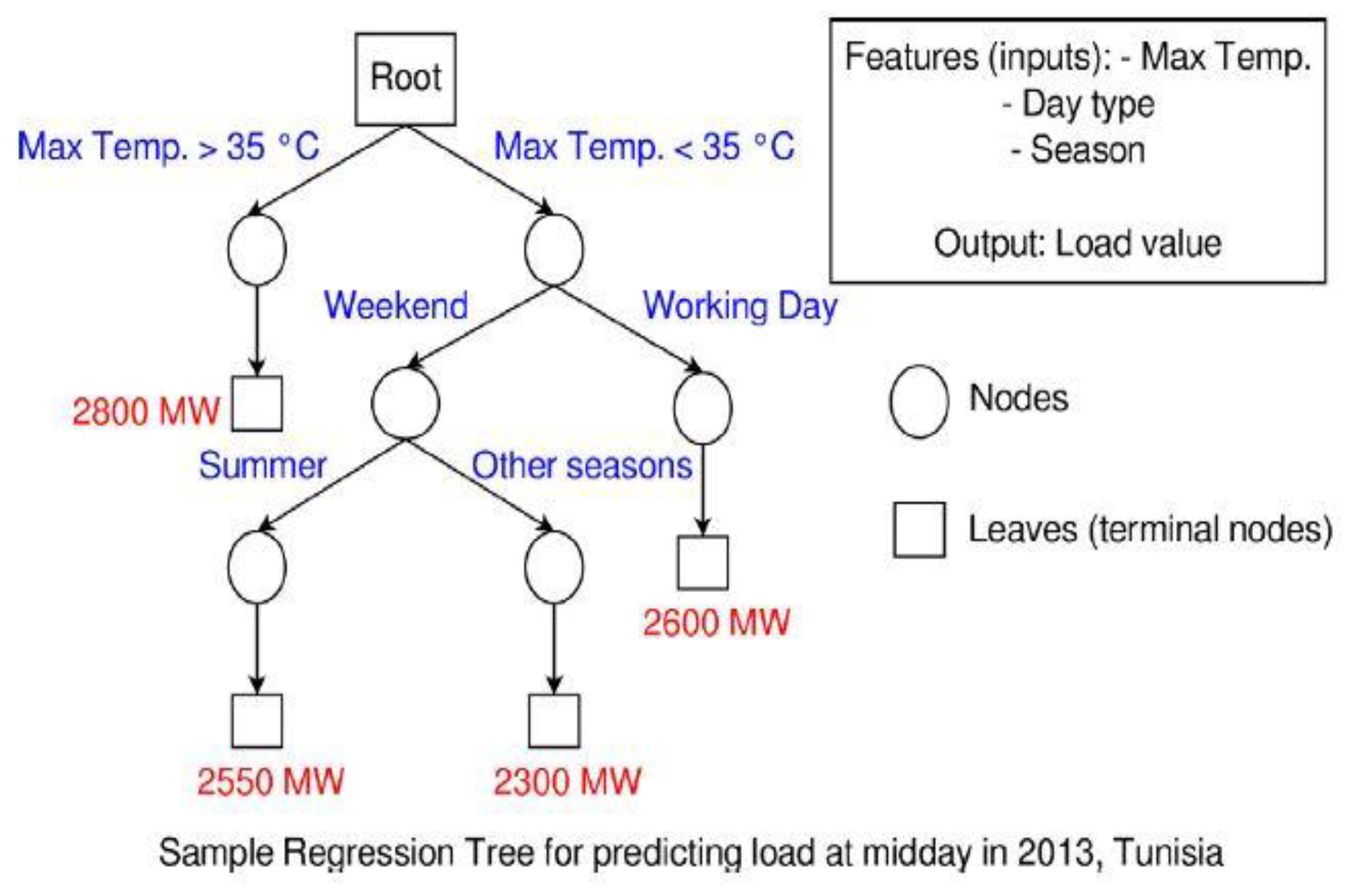
3.2.4. Decision Tree (DT)

DT, or classification and regression tree (CART), is a statistical model for solving classification and regression problems that was introduced by Breiman. The general definition of a tree is a set of nodes and edges arranged in a hierarchy without loops. The split nodes of a decision tree store a test function that will be applied to the incoming data. The leaves are the final nodes. Each leaf stores the final test result, or answer. In fact this algorithm uses mathematical modeling and finds the most optimal permutations by defining a function and minimizing the cost function [129,130]. For example, if we want to use this model to predict the electrical load and we have the three factors of maximum temperature during the day, season, and type of day, then the DT model is as shown in Figure 4 [130].

Coşgun et al. reviewed data on algal biomass to evaluate its productivity using a DT algorithm. In this model, the variables related to microalgae biomass have been investigated in this way [131].

3.2.5. Random Forest (RF)

Another common algorithm in SL is one that uses a large number of DT. Therefore, the general structure of this method is based on DT method. In this algorithm, first, the number of forest trees is taken, and then, for each tree, a model is built based on the DT; among the available features, different permutations are randomly checked and analyzed and all of the combinations of the prediction are presented [132]. The classification of each permutation and checking it is called ‘bagging’ (bootstrap aggregation). It is important to note that in this algorithm, the label, which is more repetitive in training data and is more dominant, is discarded to prevent errors and other data is used with related labels and their permutations. Each tree in this forest has only one dominant feature. This algorithm can be used in binary problems, linear regression, and classification [133,134].

Zolfaghari et al. proposed an HM involving RF to generate electricity through hydropower plants [135].

3.2.6. SVM/SVR

One of the other SL algorithms that are used to analyze data in binary problems, though it can also be generalized to multi-labeled problems, is SVM. This algorithm was introduced by Vapnik in 1995 based on the structural risk minimization (SRM) principle. By minimizing the upper bound of expected risk, SRM minimizes the overall risk. Based on that, SVM minimizes the training data error. SVM can also be used for time analysis. This algorithm is used to solve the classification problem. In recent years, SVM has been applied to regression problems as well. The application of SVM in time series regression is known as support vector regression (SVR) [136,137]. SVM/SVR can be used in many problems such as regression analysis, classification, and approximation of nonlinear functions [138]. Also, this algorithm can be used in the field of pattern recognition, in which predicting electrical load is the most significant area of use [139].

Liu et al. proposed an EL model including an SVM to predict daily radiation [140].

3.2.7. Naive Bayes Classifier (NB)

This algorithm is one of the statistical classification methods that uses Bayesian classification theory. NB classifiers differ from conventional classifiers because they calculate posterior probabilities of classes instead of learning them, so they are less computationally complex and do not require training like NNs. According to Bayes’ theorem, prior probability means the original probability in the absence of any further information. Bayes’ Theorem can be explained by Equations (1) and (2):

$$P\left(A|B\right)=\frac{P\left(B|A\right)P\left(A\right)}{P\left(B\right)}$$

(1)

$$P(A|B)=\frac{P\left(B|A\right)P\left(A\right)}{P\left(B|A\right)\ast P\left(A\right)+P\left(B|-A\right)\ast P\left(-A\right)}$$

(2)

In Equations (1) and (2), $P\left(A\right)$ represents the probability of $A$, $P\left(B\right)$ represents the probability of $B$ without having knowledge about event $A$, $P\left(A|B\right)$ is the posterior probability of $A$ based on $B$, $P\left(B|A\right)$ is the posterior probability of $B$ based on $A$, $P\left(-A\right)$ is the probability of $A$ being false and the $P\left(B|-A\right)$ represents the probability of $B$ given A is false. It is based on the assumption that the effect of each feature on a class is statistically independent of all other features. These assumptions are made to simplify computation by assuming class conditional independence [141].

Montesinos et al. developed an automated cloud classification model in which Bayesian network classifications are applied to satellite imagery to optimize solar systems [142].

3.2.8. K-Means

The K-means clustering method is an iterative clustering analysis algorithm and was first proposed by Lloyd in 1957. This algorithm belongs to USL and is widely used in the field of data analysis due to its simplicity and high efficiency. K-means takes k as input parameter and divides m object sets into k clusters, making the similarity of the same cluster high and the similarity of different clusters low. The aim of the K-means algorithm is to divide data points within certain dimensions into k clusters so that the within-cluster sum of squares is minimized. In the method, k objects are randomly selected as the initial clustering center, the distance between each object and the initial clustering center is calculated, and it is assigned to the nearest clustering center. Clustering centers and the objects assigned to them represent a class cluster. For each object allocated, the cluster center will be recalculated according to the existing objects in the cluster. The loop does not end until the cluster center no longer changes or no data has been reassigned to a different cluster [143,144].

4. Deep Learning (DL)

DL has been brought to a separate section for further attention due to expansion and advancements as well as the many algorithms that have been developed based on it, but in general, it is a branch of ML. DL is a set of algorithms that can solve complex problems by imitating the structure of the human brain.

4.1. DL Algorithms

ANN is the most common algorithm for DL, but CNN, Recurrent Neural Network (RNN), Wavelet Neural Network (WNN), Deep Belief Neural Network (DBN), Radial Basis Function (RBF), etc. are algorithms that also fall into this category. DL models have shown that they have more accuracy and efficiency in prediction based on unstructured data compared to ML algorithms [145,146].

4.1.1. Artificial Neural Network (ANN)

ANN imitates the structure of the human brain, which is made up of a large number of neurons and can process vast amounts of information [147]. To build an accurate and efficient model, we need a set of parameters. In each case, we have the input data and we are looking to obtain the output data. Input data are considered as nodes in the input layer and the output data are considered as nodes in the output layer. In ANN structure, one or more hidden layers must be considered between these two layers, which include a large number of nodes that connects the input layer nodes to the output layer nodes. When data is transferred from one node in one layer to another node in another layer, it is multiplied by a specific weight factor (weight & bias values) to apply the effect of each of the input parameters in the problem-solving process. Single layer perceptron (SLP) is the simplest type of ANNs and can only classify linearly separable cases with a binary target. An SLP is a feed-forward network based on a threshold transfer function. In contrast, a multilayer perceptron (MLP) is a feedforward ANN that generates a set of outputs from a set of inputs. An MLP is characterized by several layers of input nodes connected as a directed graph between the input and output layers. MLP uses back propagation (BP) for training the network. These models are very efficient and accurate in predicting test data and nonlinear problems [148,149,150]. Figure 5 shows an image of an ANN with a hidden layer [151].

It should be noted that if the number of hidden layers or the number of nodes in them is high, the problem becomes an overfit and will no longer have the necessary performance [152]. Since the learning process is performed on training data and examined on test data, after obtaining the answer, it is compared with the real answer and optimized by the loss function. In this way, the obtained value is compared with the actual value, the difference is considered, and then the process is performed in the opposite direction to correct the assigned weights to reduce the difference; these steps are repeated until the desired result is reached, this process being BP [153]. The optimization process is performed by returning to the input data and modifying the weight & bias values. In Table 2, some common activation functions are introduced, which are further explained in Activation Function in Section 4.1.2.

Jahirul et al. used a model involving ANN to analyze the relationship between chemical composition and biodiesel properties to find the main components [154]. Huang et al. proposed a multivariate hybrid DNN model to accurately predict solar radiation for efficiency in electrical energy management and planning [155].

Table 2. Types of activation functions used in NN [137,156,157].

Name of the Activation Function	Formula	Graphical Representation	Number of Equations
Linear	$f\left(w\right)=w$		(3)
Sigmoid	$f\left(w\right)=\frac{1}{1+e^{-w}}$		(4)
Hyperbolic tangent sigmoid (tanh-sig)	$f\left(w\right)=\tan \mathrm{h}\left(w\right)=\frac{e^w-e^{-w}}{e^w+e^{-w}}$		(5)
Binary step	$f\left(w\right)=\{\begin{array}{c} 1 w>0\\ 0 w\le 0\end{array}$		(6)
Rectified Linear Units (ReLU)	$f\left(w\right)=\{\begin{array}{c}w for w\ge 0\\ 0 for w<0\end{array}$		(7)
Leaky ReLU	$f\left(w\right)=\{\begin{array}{c}w for w>0\\ aw for w<0\end{array}$		(8)
Exponential Linear Unit (ELU)	$f\left(w\right)=\{\begin{array}{c}w for w>0\\ a\left(e^w-1\right) for w<0\end{array}$		(9)
Gaussian Radial Basis	$f\left(w\right)=exp \left(\frac{-\Vert w-\omega \Vert }{2{\sigma }^2}\right)$		(10)
Softmax	$\sigma {(\overrightarrow{z})}_i=\frac{e^{z_i}}{{{\displaystyle \sum }}_{j=1}^k{e}^{z_j}}$		(11)

Table 2. Types of activation functions used in NN [137,156,157].

Name of the Activation Function	Formula	Graphical Representation	Number of Equations
Linear	$f\left(w\right)=w$		(3)
Sigmoid	$f\left(w\right)=\frac{1}{1+e^{-w}}$		(4)
Hyperbolic tangent sigmoid (tanh-sig)	$f\left(w\right)=\tan \mathrm{h}\left(w\right)=\frac{e^w-e^{-w}}{e^w+e^{-w}}$		(5)
Binary step	$f\left(w\right)=\{\begin{array}{c} 1 w>0\\ 0 w\le 0\end{array}$		(6)
Rectified Linear Units (ReLU)	$f\left(w\right)=\{\begin{array}{c}w for w\ge 0\\ 0 for w<0\end{array}$		(7)
Leaky ReLU	$f\left(w\right)=\{\begin{array}{c}w for w>0\\ aw for w<0\end{array}$		(8)
Exponential Linear Unit (ELU)	$f\left(w\right)=\{\begin{array}{c}w for w>0\\ a\left(e^w-1\right) for w<0\end{array}$		(9)
Gaussian Radial Basis	$f\left(w\right)=exp \left(\frac{-\Vert w-\omega \Vert }{2{\sigma }^2}\right)$		(10)
Softmax	$\sigma {(\overrightarrow{z})}_i=\frac{e^{z_i}}{{{\displaystyle \sum }}_{j=1}^k{e}^{z_j}}$		(11)

4.1.2. Convolutional Neural Network (CNN)

Due to the continuing development of NNs, and also the requirement to solve new problems and challenges, these types of NNs have a special application. CNNs have become very popular in image-related projects due to their optimal performance and high accuracy results, but have other applications too, such as speech recognition, image classification, image recognition, autopilot vehicles, and so on [158,159].

Zhou et al. developed a model based on this type of network for fault detection in gas turbines [160]. Imani et al. proposed a model based on CNN, using hourly electrical load and the nonlinear relationship between the load and energy consumption, as well as the the associated temperature to predict electrical load demand in the residential sector [161].

In general, CNNs have a specific structure and actions as follows, among them the input layer, activation function, back propagation, feed-forward, and loss function, which also exist in basic ANN.

Input Layer

The data is given to the model through input layers. In any network, the input layer is the first and one of the most important steps.

Convolutional Layer

The core of a CNN is where most of the necessary calculations are made. Each convolutional layer contains a set of filters that the output of the convolution layer (feature map) is obtained through the convolution between the filters and the input layers. In general, more layers means more filters, a deeper network and more accurate results [158].

Pooling Layer

The purpose of these layers is to reduce the size of the feature map obtained in the previous step. It is also used to reduce the number of parameters and to prevent overfitting, and also to eliminate unwanted noise. The process is to move a specific frame on the image and sample it so that it calculates the value of the new parameter in each navigation using mathematical operations. The pooling operation is performed in two ways: max pooling and average pooling. These steps operate on the pixels of the image, and in each step, depending on the type of pooling operation, the maximum value or the average number corresponding to the pixels results in reducing the dimensions [162].

Activation Function

The activation function specifies the output of the neurons. The weighted sum of the input values of the linear network is transferred to the activation function to convert it to a nonlinear function. This step aims to maintain the features and eliminate some extra features, the most important abilities of CNNs in solving nonlinear problems. It should also be noted that one of the most widely used nonlinear activations in fully connected layers is the ReLU function, although the softmax function is employed as an activation function of an output layer [163]. Some types of activation functions used in NNs, especially softmax, are given in Table 2. It is suggested to those interested to refer to the mentioned references for more details regarding each activation function [137,156,157].

In Equation (11): i = 1, 2…, k, $\sigma$ represents softmax, $\overrightarrow{z}$ is input vector, $e^{z_i}$ is the standard exponential function for input vector, k is number of classes in the multi-class classifier, $e^{z_j}$ is the standard exponential function for the output vector [157].

Fully Connected Layer (FCL)

In general, the last layers of a CNN for classification are these types of layers. The most important application of these layers in the CNN is use as a classifier. The set of properties extracted using convolutional layers are eventually transformed into a vector. Finally, this attribute vector is given to a fully connected classifier to identify the correct class [160,163].

Loss Function

This function is used to estimate the deviation of the predicted value from the actual value. The lower the value of this function, the greater the accuracy of the proposed model. Therefore, this function plays a very important role in optimizing the model and increasing its accuracy. Equation (12) displays the general form [158].

$$L\left(Y,F\left(x\right)\right)=\left|Y-F\left(x\right)\right|$$

(12)

In Equation (12): $Y$ represents the actual value and $F\left(x\right)$ represents the value calculated by the CNN.

Back Propagation and Feedforward

In a CNN, a random weight is first multiplied by each of the inputs. In the next step, the activation function is applied to each of the said items and their value is changed. In the end, the output is taken according to the previous cases and the value of the loss function is calculated. These steps are called feedforward steps. Due to the error and deviation of the mentioned cases from the values of the training data, the feedforward step is conducted in reverse to change the values of the weights assigned to each of the inputs, in order to increase accuracy and reduce error. The feedforward step is performed again to evaluate the results. The set of steps mentioned is the same as BP described in Section 4.1.1. Figure 6 shows the outline of a CNN model with numerous CLs and PLs performed alternately, as well as fully connected layers and a softmax layer as the classifier [164]. The study of the mathematical relationships of CNNs is beyond the scope of this article and therefore can be referred to [160,163,165].

Alves et al. examined the impact of data utilization techniques to enhance CNN performance for classifying anomalies in PV modules [166].

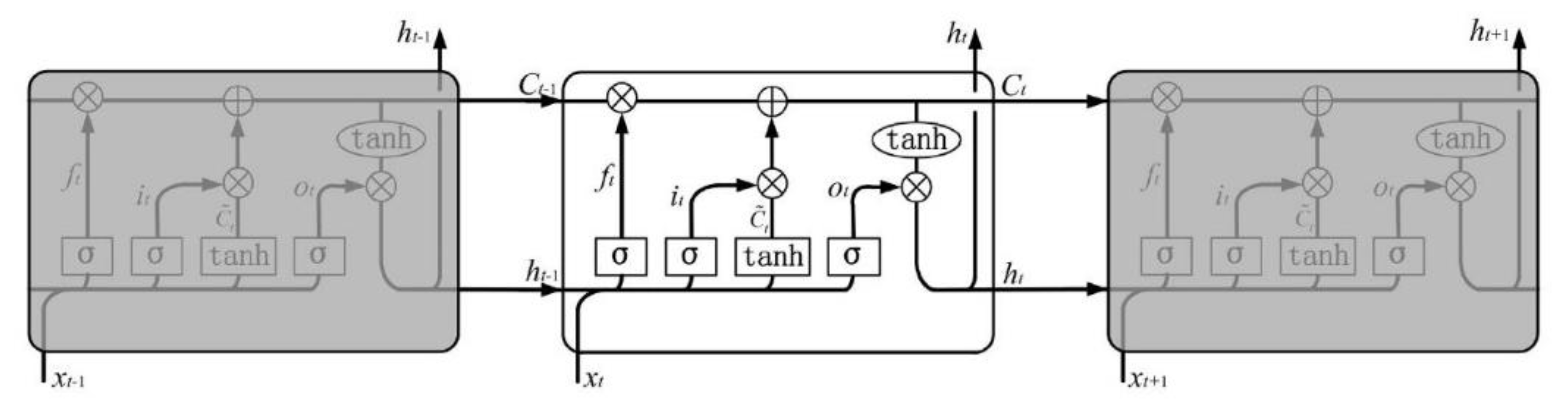
4.1.3. Recurrent Neural Network (RNN)

Another type of NN used in DL is RNN, which is used in matters where the data sequence is important, such as language translation or electrical load prediction. The consecutive connection of neurons in the past, and with their internal state, provides the basis for modeling time problems so that these types of networks are also related to past outputs. In general, RNN is designed so that the process of BP takes place over time, and such a feature for models with very large sequences causes them to forget the previous data. To solve this problem, the LSTM model has been developed, which enables the model to store data for longer periods and make more accurate predictions. As the main part of the recurrent hidden layer of the LSTM, there are special units called memory blocks which lead to the storage of data over extended periods of time. In addition, there are three multiplicative units for managing the flow of information, namely the input gate, forget gate, and output gate around each LSTM cell, forming a new computing unit. The input information is controlled by the input gate, the saving of the computation unit’s past status information is made by the forget gate, and the information output is controlled by the output gate. Thus, it can be said that such networks are an improved type of RNN [167,168].

Figure 7 shows the internal structure of RNN [169]. Figure 8 shows the outline of LSTM, in which, $c_t$ denotes the calculation rules of LSTM cells at time t, $h_t$ is the output of the calculation unit at time t, W, U and V denote the parameter matrices, and b is the bias vector. $i_t$, $f_t$ and $o_t$ denote the input, forget, and output gates and the cell state vector at time t. It is clear that the input, forget and output gates are respectively connected to a multiplicative unit to control the input and output of information and the state of each LSTM cell. $\otimes$ represents element-wise multiplication. In addition, activation functions are mentioned in Table 2 [169].

Sun et al. proposed an LSTM-based RNN for power prediction in real power plants for turbine evaluation [170]. Pang et al. proposed an ANN model and an RNN to investigate ML algorithms for predicting solar radiation [171]. Agga et al. used an HM including LSTM to predict the production capacity of a PV power plant [172].

4.1.4. Restricted Boltzmann Machine (RBM)

RBM machines are a special type of generative energy-based model. Generative Models (GMs) learn an underlying data distribution by analyzing a sample dataset. Structurally, the RBM is a shallow neural network with only two layers—the visible layer and the hidden layer. In this network, each node is connected to all nodes in the adjacent layer and represented by an undirected fully connected graph. The term restriction refers to the fact that no two nodes in a layer are related to each other. RBM is the mathematical equivalent of a two-way translator and the standard type of RBM has binary-valued hidden and visible units. In the forward pass, the RBM takes the inputs and converts them to a set of numbers that are the encrypted state of the inputs. In the backward pass, it takes the set of numbers and translates them to obtain the early input. A well-trained network will be able to translate back with a high accuracy. Weights and biases are very important in both stages. They allow the RBM to decode the interrelationships between the input attributes, and they also help the RBM decide which input attributes are the most important when identifying patterns. An RBM is trained to reconstruct the input data through several forward and backward movements. The interesting aspect regarding RBM is that the data does not need to be labeled. This is very important for real-world data sets such as photos, videos, audio and sensor data, and all items that tend to be unlabeled. Instead of people tagging data manually and reporting errors to the system, an RBM automatically sorts the data, and by setting the weights and bias correctly, the RBM is able to extract important features and reconstruct the input. Those who are interested can also refer to the mentioned references for more details and equations related to this model [173,174,175]. The structure of this model is shown in Figure 9 [174].

Yang et al. proposed an unsupervised model for detecting anomalies in the monitoring system of wind turbines including RBM [176].

4.1.5. Auto Encoder (AE)

AE is generally known as a feature extraction algorithm in the case of USL problems. It is a type of symmetrical NN that is used to optimize learning. Instead of training the network and predicting the target value of y, for x input, the AE model is trained to reconstruct the input value of x, so the output value will be the same as the value of x [177]. This algorithm can extract properties with the least amount of reconstruction error (RE). As mentioned in Equation (13) and Figure 10, the AE network reconstructs the same value for input x and delivers it as output [178,179].

$$\mathrm{y}={\mathrm{f}}_{\mathrm{AE}}\left(\mathrm{x}\right)=\mathrm{x}$$

(13)

It should be noted that during the process, the model is optimized by minimizing the RE value [180]. Figure 11 provides an overview of the process of performing AE.

Qi et al. designed a variable AE model to evaluate and describe uncertainties in power systems and to examine possible scenarios [181]. Renström et al. proposed an AE-based model that reconstructs all its input signals to detect widespread anomalies in wind turbines [179].

4.1.6. Deep Belief Neural Networks (DBN)

DBN is another NN that the network serves as a graphical model, introduced by Hinton, and learns to extract deep hierarchical representations of the input data [173,182]. In general, this type of network consists of a USL pattern and a large number of RBMs and LOR, which RBM uses to identify and extract features, and LOR to predict [183].

Hao et al. developed a model based on this type of network to predict the energy consumption required by the calcination process for cement production [184]. Sun et al. used a new efficient method to optimally identify proton exchange fuel cell cells based on an improved version of a DBN [185]. Figure 12 shows the structure of a DBN instance with RBMs inside it [186].

4.1.7. Generative Adversarial Network (GAN)

Another type of NN is very powerful and popular, which was introduced in 2014 by Ian Goodfellow. This type of NN consists of two parts, the GM and Discriminator Model (DM). The task of the first part is to generate new data based on past data, while the task of the second part is to examine and distinguish between the actual data presented and the generated data. Some of the applications of these networks can be considered as reducing the noise in images or producing human images. Figure 13 shows the general structure and also the implementation process of this type of network. In CNN, GM and DM compete with each other so that the model can produce the desired result. Finally, there is a loss function to optimize results by performing the BP process, similar to that mentioned in Section 4.1.1 and Section 4.1.2. It should be noted that each of the two parts, GM and DL, is performed by two separate NNs [187,188,189,190].

Wang et al. used a generalized model based on GAN as EL to predict the distributed surface pressure distribution on gas turbine blades [191].

4.1.8. Adaptive Neuro-Fuzzy Inference System (ANFIS)

Fuzzy systems are a common computational method based on fuzzy theory and its rules and logic [192]. If NNs and fuzzy theory are combined, a powerful network will be created that will both use NN rules and have a logic based on fuzzy theory. In neuro-fuzzy systems, the weight coefficients in the NN are determined based on fuzzy equations [193]. ANFIS can be used for classification, approximation of highly nonlinear functions, online identification in discrete control systems and to predict a chaotic time series. ANFIS can serve as a basis for constructing a set of fuzzy ‘if–then’ rules with appropriate membership functions to generate the stipulated input-output pairs. ANFIS is based on the Takagi-Sugeno model [194,195]. The Takagi-Sugeno systems are one of the most common fuzzy models. In such systems, consequents are functions of inputs. They use a rule structure that has fuzzy antecedent and functional consequent parts [196].

Figure 14 shows an example of the structure of such networks, which contain five layers with different functions. The following is a description of each layer’s function. The main purpose of layer one is to map input variables into fuzzy sets through the process of fuzzification. This layer’s nodes are square nodes with node functions that generate membership grades. In layer two, after integrating the fuzzy sets of each input, the firing strength will be used. The output is obtained using the G-norm operator, which performs the fuzzy conjunction “and”. The primary goal of layer three is to calculate the ratio of the ith rule, the firing strength to the sum of all firing strengths. In layer four, the output from layer three is multiplied with the function of the Sugeno fuzzy rule. In layer five, there is only one node. This single node computes the sum of all the outputs of each rule from the previous layer. Next, we perform the process of defuzzification by using the weighted average method, which converts the fuzzy result into a crisp result. It is suggested to refer to the mentioned reference for more details regarding this structure [195,197].

Ammar et al. proposed a model based on ANFIS to show the accuracy and importance of ANFIS for optimizing maximum output power in PV systems. [198].

4.1.9. Wavelet Neural Network (WNN)

This is a type of NN based on wavelet transforms and based on deep multilayer NN as an alternative to ANN [199]. In this type of NN, the discrete wavelet-based function is considered as the activation function for each node and generally has better results than ANNs with the same number of layers and neurons. This type of NN is faster due to the use of a discrete wavelet-based function [200]. The inputs to the WNN and forecasted outputs are shown by $c_i$ and $y_k$, respectively. The weights of the data association between the input layer and the hidden layer are shown by $w_{ij}$, and Equation (14) shows the results of the hidden layer.

$$\begin{gathered} h\left(j\right)=h_j\left(\frac{{{\displaystyle \sum }}_{i=1}^d{w}_{ij}{c}_i-b_j}{a_j}\right) \\ j=1,2,3,\dots ,l \\ i=1,2,3,\dots ,l \\ k=1,2,3,\dots ,m \end{gathered}$$

(14)

In Equation (14): $h\left(j\right)$ represents the result of the $jth$ hidden layer node, $a_j$ represents scaling parameter of the wavelet-based function, $b_j$ defines an interpretation parameter for a wavelet-based function, $l$ is the number of neurons that are in the hidden layer and $h_j$ is the wavelet-based function. The final result of WNN is given in Equation (15) [201]:

$$y_K={\displaystyle \sum }_{i=1}^l{w}_{ik}h\left(j\right)$$

(15)

Yuan et al. developed a WNN-based method for predicting midterm electrical energy consumption in buildings on two numerical items [201]. Aly et al. proposed an HM for predicting harmonic tidal currents based on clustering approaches to improve the accuracy of the related systems [202].

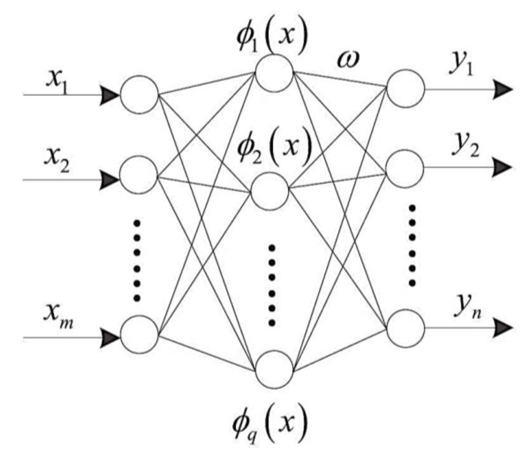
4.1.10. Radial Basis Neural Network (RBNN)

RBNN is a three-layer NN that contains a hidden layer that can learn quickly and can be used in nonlinear continuous functions. Figure 15 shows the general structure of an RBNN [203,204]. This type of NN is based on ANN, in which the Radial Basis Function of the type of the Gaussian function is used as the activation function. In general, the equation of a Gaussian function is Equation (16). Equation (17) represents the Radial Basis function and Equation (18) represents the value of the radial basis function multiplied by the assigned weight factor [205].

$$\mathsf{\varphi }\left(x\right)=\exp \left(-\frac{x^2}{{\sigma }^2}\right)$$

(16)

$$g\left(x\right)=\exp \left(-\frac{{\Vert x-{\beta }_k\Vert }^2}{{\sigma }_k{}^2}\right)$$

(17)

$$f\left(x\right)={\displaystyle \sum }_{i=1}^n{w}_i{g}_i\left(x\right)$$

(18)

In Equation (16): $\sigma$ is the radius of the Gaussian function. In Equation (17): ${\beta }_k$ is the center of the function, and ${\sigma }_k$ is the radius of the function. In Equation (18): $w_i$ is the weighted coefficients assigned and $g_i\left(x\right)$ is the output of the radial basis function in Equation (17).

Hussain et al. designed an RBNN with two inputs for fault detection in PV systems [206]. Karamichailidou et al. designed a model based on an RBNN to model the wind turbine power curve using wind speed, wind direction, ambient temperature, and blade pitch angle as input parameters, achieving accurate and appropriate results [207].

4.1.11. General Regression Neural Network (GRNN)

This type of network, which is used in regression and in classification, can be considered as a normalized type of RBNN, in which there is a centralized unit in each training process. However, unlike RNBB, it does not require BP. In general, in this type of network, an arbitrary function of training data is approximated [208]. GRNNs have four layers, including the input layer, output layer, pattern layer, and summation layer. The input of the pattern layer is the output of the input layer and the pattern layer is connected to the summation layer. The output layer and the summation layer work together to normalize the output vector of the network. In the learning process, both in the hidden layers and the output layer, linear and radial basis functions are used as the activation function [209,210].

Sakiewicz et al. designed an HM including GRNN to predict three types of biomass ash melting temperatures [211].

4.1.12. Extreme Learning Machine (ELM)

ELM is a technique for practicing NN data such as the Single Hidden Layer Feed-Forward Neural Network (SLFN), which was introduced in 2006 by Guang-Bin Huang et al. [212]. It is very similar to RBFN and its structure is similar (both consist of an input and output layer and a hidden layer). The difference is that in RBFN, all neurons are assigned a single weight between the input layer and the hidden layer, but in ELM, a small weight is initially randomly assigned. This type of network has a faster learning speed than RBFN and CNN [213].

Shamshirband et al. used this technique to predict horizontal solar radiation [214].

4.1.13. Ensemble Learning (EL)

EL is a model that consists of a large number of ML algorithms and is used to study and analyze a specific goal [215]. In other words, several ML methods are taught in parallel for a single purpose, so that the performance of each is compared and each should have a lower amount of uncorrelated error (UE) [216]. EL is one of the most common methods in statistical topics and ML. In general, fast learning methods such as RF and DT are used in this type of model. Slower learning methods can also be used in this type of learning. It should be noted that performing computational operations for EL may be a little time-consuming, but this can be compensated by the weak accuracy and results of slow methods [217]. One can refer to [218] for further details. The following are the different types of EL methods. Figure 16 outlines this type of learning.

Boosting

Boosting is an EL method that uses weak classification methods, such as DT, and optimizes the loss function step by step [217]. In this method, the classifiers are combined and the sample weights are considered repeatedly, while weights are adjusted step by step to increase the weight in question to the items used in the previous step. Finally, the final predictions are obtained by weighting the results produced [219]. The general basis of this algorithm is that a large number of simple algorithms will have better performance than a complex algorithm; however, we will face the problem of a high bias value in the results. Therefore, as the name of this method indicates, by reducing the bias value, it makes it possible for us to use this method [220]. This method also includes AdaBoost, XGBoost and AdaBoost.MRT, each of which is discussed below.

Li et al. developed an HM of this method to predict wind speed in several stages in. order to discover the power of wind power generation [221].

Adaptive Boosting (AdaBoost)

AdaBoost is one of the most common boosting methods, introduced by Freund in 1995 [222]. The algorithms used in it are executed sequentially. As shown in Figure 17, training data is first used as the first data set. In the next step, Algorithm No. 1 is executed upon it and the preliminary results are obtained. Next, the algorithm is evaluated according to test data and a weighting factor is given to the algorithm according to the accuracy of the results obtained. Then, those data that were not correctly predicted by this algorithm proceed to the next section as a data set, so that the next algorithm can be tested with them and the mentioned steps are repeated. Thus, in AdaBoost, at each stage, each algorithm tries to complete and strengthen the previous algorithm to optimize the results. Finally, based on the assigned weight coefficients $W$, the final processing is performed and presented to obtain the best and most accurate method [221,223,224].

Wang et al. designed a model based on the EL method, based on AdaBoost, to predict electrical energy consumption in the industrial sector in China [225].

Extreme Gradient Boost (XGBoost)

XGBoost was introduced by Chen [226]. In this method, weak algorithms are combined to create a powerful model. Despite the simplicity and volume reduction in the calculations, the results are very accurate [227]. This algorithm is based on gradient amplification so that its purpose is to reduce the loss function using the idea of a descending gradient. XGBoost is widely used in classification and regression problems [228]. In order to read more details, one can refer to [228].

Wei et al. developed a model based on some of the most common ML algorithms, including XGBoost, to predict the residential district heating load in Shanghai, China, based on data from electrical, thermal, and meteorological sensors [229].

AdaBoost.MRT

If the output of the problem involves several variables (vectors), the classical AdaBoost algorithm must be generalized to be able to solve the problem in this situation. The general approach in this algorithm, as in the previous cases, is to integrate simple and weak algorithms to increase the accuracy of problem-solving [230]. To read more details, one can refer to [221,231].

Liu et al. developed a model based on EL, including this algorithm, to predict the air quality index and pollution in China [232].

Bagging

Bootstrap aggregating, also known as bagging, was introduced in 1996 by Breiman. He has stated that grouping decision and regression trees yield much better results than individual trees [233]. An example of this approach is the RF method, the contents of which were mentioned in the relevant section [234]. This method is used in statistics and regression-based classifications where the data have high variance or there is a large amount of data. Here, a type of averaging is conducted in the model and the overall goal is to increase the stability and validity of other ML algorithms [235]. The important point is that the basis of all the algorithms used must be the same (such as kNN, ANN, NB, DT). The main purpose of this method is to use complex ML algorithms in a way that avoids overfitting [236].

Oliveira et al. developed an EL model including this method for predicting electricity consumption based on electrical energy data from various countries [237].

Stacking

Stacked Generalization, or stacking, is a method in which, for each of the ML algorithms, according to its importance and accuracy, a weighting factor is supposed to consider the impact of the importance and power of each algorithm in the final results. In the end, the results are grouped by the weighting coefficients assigned in the final model and the overall result is presented [238,239].

Ngo et al. proposed an alternative model based on ensemble bagging and stacking ANNs to predict cooling loads of buildings with few common parameters in the design phase [240].

4.1.14. Hybrid Model (HM)

In general, if the mentioned algorithms are combined in series, reviewing the data in this way can increase the accuracy and efficiency of the analysis to an acceptable level. Thus, using an HM, we can predict the desired parameters by combining different algorithms and analyzing the results together [155,241].

Zhang et al. used an HM involving several ML algorithms, especially DL algorithms, to accurately and reliably predict wind speeds for the development and management of wind power generation systems [241].

4.1.15. Transfer Learning (TL)

If the data and learning experiences of one model are transferred to other models for use in new learning, several models will use shared learning experiences and data [242]. The purpose of TL is to improve learning performance to achieve greater accuracy in the results obtained [243,244]. Figure 18 shows an overview of TL.

Hu et al. proposed a TL-based method using wind data from the region’s older wind farms to predict the wind power of a newly established power plant [245].

5. Time Series (TS)

A TS is a set of time data recorded at equal intervals and specified. Time data analysis is divided into two parts. The first part is related to identifying the structure and pattern of the given data and the second part is related to fitting a model to predict the future trend. TS analysis is used for many applications, including economic forecasting, processing and quality control, census analysis, and so on. A TS can be univariate or multivariate. If there are several target variables, the problem is multivariate. One of the important applications of univariate TS in energy systems is the analysis and prediction of energy consumption over time [22,246].

5.1. TS Algorithms

The TS has important algorithms such as moving average (MA), exponential smoothing (ES), autoregressive moving average (ARMA), case-based reasoning (CBR), etc., which are explained below. In addition, LSTM, as one of the DL algorithms, as mentioned before, has been widely used in predicting TS with high accuracy due to the observance of time data sequences.

5.1.1. Moving Average (MA) & Exponential Smoothing (ES)

ES & MA are two distinct forecasting methods, but they have one thing in common: they both consider the TS locally stationary over the local period. Despite this, ES gives a higher weighting to recent values whereas MA gives equal weighting to all values. The MA assumes that observations close to each other in time are likely to have similar values in the future. Many TS analysis techniques derive their basic underlying foundation from these decomposition components [22]. The MA written in Equation (19) is a simple equally weighted calculation.

$${\widehat{Z}}_{t+1}=\frac{Z_t+Z_{t-1}+\dots +Z_{t-m+1}}{m}$$

(19)

In Equation (19): The average is centered at period $\frac{t-\left(m+1\right)}{2}$ and, at time $t+1$, ${\widehat{Z}}_{t+1}$ represents the forecasted value of $Z$, which is calculated at the moment $t+1$, equal to the simple average of the recent observations $m$ at time $t$.

By applying greater weights to more recent observations, ES is accomplished. Weighted averages are used to calculate forecasts, which decrease exponentially as observations are taken further into the past. The proposed concepts can be modeled mathematically as Equations (20) and (21) [22].

$$S_t={\widehat{Z}}_{t+1|t}=a{Z}_t+\left(1-a\right)S_{t-1}=S_{t-1}+a\left(Z_t-S_{t-1}\right)$$

(20)

$${\widehat{Z}}_{T+h|t}=S_T$$

(21)

In Equation (20): $S_t$ represents the estimation of the level at time $t$, $Z_t$ is the observed TS at time $t$, ${\widehat{Z}}_t$ is the forecasted value of $Z_t$ at time t and $a$ is the parameter related to the smoothing of the level that can be chosen from ($0<a<1$). In the case of $a$ close to 1, the forecast becomes very sensitive to swings in previously recorded values based on the previous period’s error.

In Equation (21): The T-index represents the periodicity obtained in the data utilized in the variables and the concepts of other variables are similar to the variables in Equation (20). One can refer to [247] for further details.

Cadenas et al. analyzed wind data from a temporal perspective through ES, and then compared the results obtained through EL with the results obtained through ANN [248].

5.1.2. Autoregressive Moving Average (ARMA)

This algorithm is a combination of MA and AR. AR concentrates on movement and trend patterns, while MA records the effects of white noise. This method is a statistical method that allows us to predict the behavior of TS. Equations (22) and (23) represent the mathematical formulation of ARMA [22].

$${\widehat{x}}_t=c+{ϵ}_t+{\displaystyle \sum }_{i=1}^n{\phi }_i{x}_{t-i}+{\displaystyle \sum }_{i=1}^m{\theta }_i{ϵ}_{t-i}$$

(22)

$$e_t=x_t-{\widehat{x}}_t$$

(23)

In Equation (22): $x_t$ is related to the actual value of $x$ in time $t$, ${\widehat{x}}_t$ is the forecasted value of $x_t$ through this algorithm, and ${ϵ}_t$ represents the additional factors. In $ARMA\left(n,m\right)$, n is related to the order of AR and $m$ is related to the order of MA, while ${\phi }_i$, ${\theta }_i$ are related to the effect of previous errors and predictions on subsequent predictions.

In Equation (23): $e_t$ represents the prediction error performed. It should be noted that the value of $\left(n,m\right)$ can be calculated according to the data [249,250].

The validity of the predicted data is checked using the Akaike Information Criterion (AIC), formula given in Equation (24).

$$AIC=logA+\frac{2c}{n}$$

(24)

In Equation (24): $A$ represent the value of loss function, c represents the number of estimated parameters and n is related to the total data that exist in the dataset [251]. It should also be noted that the validity of the model can be calculated through the formulas in Section 6.

Zhang et al. developed a model including ARMA to achieve spatial-temporal correlation between wind and solar power plants. They obtained a joint distribution for wind and solar power plants and considered the relevant scenarios [252].

5.1.3. Autoregressive Integrated Moving Average (ARIMA)

ARIMA, or BOX-Jenkins, is another statistical algorithm for predicting data behavior based on AR and MA. The term ‘integrated’ refers to a separation step used to eliminate the trend or periodicity of a TS [253]. In general, ARIMA parameters are similar to ARMA, except that it is specified as $ARIMA \left(n, d, m\right)$. Parameter $d$ represents the number of periods that need to be integrated to be fixed. The mathematical Equation of $ARIMA \left(n, d, m\right)$ is similar to Equations (22) and (23). The difference between ARMA and ARIMA is that ARMA is used for fixed TS, whereas, if our TS is not fixed, it needs to be integrated, in which case we must use ARIMA.

Some examples of the application of this method are: predicting the trend of the daily air purity index [254], forecasting wind speed in the coming days [255,256], predicting sunlight and its fluctuations during the day [257], forecasting hydropower energy consumption [33], and analyzing energy supply and demand trends.

5.1.4. Case-Based Reasoning (CBR)

CBR is a method of combining learning and problem-solving methods and is based on retrieving past information about a case to solve a new case. In general, this method is based on past observations and tries to model new cases based on past scenarios. The resource needed for learning is a memory of previously stored records. The basis of this method is the role of reminders in human inference [22,258]. Learning in this type of system is related to the structure within it, which consists of four key stages. Retrieve, reuse, revise and retain (4R) refer to retrieving past similar cases, reusing methods from similar cases to provide a possible solution to a new problem, revising the solution if necessary, and retaining the new solution by placing it at the basis of the solution method for solving similar cases in the future. CBR has been widely used to build information archives for science management and decision making. Figure 19 shows the operation process of this method [259].

Koo et al. used an advanced CBR-based ML model to study solar radiation in China due to the complexity of patterns and relationships in the region’s solar data, using data from 2006 to 2020, and achieving very good results [260].

5.1.5. Fuzzy Time SERIES (FTS)

FTS that are modeled with values corresponding to linguistic variables cannot be analyzed by the rules and relationships common to other TS. Song et al. (1993) introduced this type of series [261]. The important aspect is choosing the appropriate fuzzy distance length, which has a great impact on the accuracy of the results. Providing more content in this area is beyond the scope of this article; one can refer to [261,262] for more information.

Severiano developed a model based on FTS to predict solar and wind energy [263].

5.1.6. Grey Prediction Model (GPM)

This method was first introduced in 1982 by Deng [264]. This algorithm is used to solve discrete data uncertainty problems if there is not enough data available. The main application and purpose of this method are to predict the future of systems that cannot be studied and predicted by fuzzy methods or limited data. In this method, there is no need to know the probability distribution of the input data. One of the general advantages of this method is the possibility of using it in cases of limited data. In general, this method is based on a set of first-order differential equations [265]. For more details about this method and its equations, one can refer to [266,267].

Duan et al. used a new multivariate GPM model to predict energy in China based on the energy logistics equation [268].

5.1.7. Prophet Model

The Prophet prediction model was introduced by Facebook in 2017. The prophet is a method for predicting TS data in which nonlinear trends are predictable in daily, weekly, and annual periods. This algorithm was originally designed for use in business forecasting, but due to its high ability to analyze various trends, it can be used for forecasting renewable energy [269,270].

Wang et al. developed an HM involving the Prophet algorithm to predict power outages and weather events [271].

6. Performance Evaluation Metrics

Since the purpose of predicting the critical parameters of energy systems is the evaluation of reliability and stability, the accuracy of the constructed model is critical. Thus, paying attention to the accuracy of the model and optimizing it to reduce errors and increase its accuracy is very important [137]. To evaluate the results of ML and DL models and evaluate their effectiveness, we must evaluate the results according to the appropriate metrics. For this purpose the following metrics can be considered: R² [272], MSE [106,113], MAE [3,106], RMSE [273,274], nRMSE_% [275], MAPE [3,113], MBE [272], t-stat [43], CV-RMSE [276].

In this section, there are many statistical evaluation metrics to examine the learning process of the model. In all these cases, the real variable and the predicted variable in the learning data are used. Thus, a brief explanation of each is given below.

6.1. Mean Squared Error (MSE)

In general, this value is defined as the mean squared of the difference between the actual data and the predicted data [4]. The MSE equation is given below as Equation (25).

$$MSE=\frac{1}{N}{\displaystyle \sum }_{i=1}^N{\left({y_{forecasted}}_i-{y_{actual}}_i\right)}^2$$

(25)

6.2. R-Squared (R²)

To evaluate the performance of linear regression models, a coefficient of determination known as $R^2$ is used. The $R^2$ equation is given below as Equation (26) [277].

$$R^2=1-\frac{ {{\displaystyle \sum }}_{i=1}^N{\left({y_{actual}}_i-{y_{forecasted}}_i\right)}^2}{{{\displaystyle \sum }}_{i=1}^N{({y_{actual}}_i-{y_{mean}}_i)}^2}$$

(26)

6.3. Mean Absolute Error (MAE)

This metric results in an absolute mean error. The MAE equation is given below as Equation (27) [278].

$$MAE=\frac{1}{N}{\displaystyle \sum }_{i=1}^N\left|{y_{forecasted}}_i-{y_{actual}}_i\right|$$

(27)

6.4. Root Mean Square Error (RMSE)

The general concept is the standard deviation of the difference between the forecast and actual data. The RMSE equation is given below as Equation (28) [279].

$$RMSE=\sqrt{MSE}=\sqrt{\frac{1}{N}{\displaystyle \sum }_{i=1}^N{\left(y_{forecasted}{}_i-y_{actual}{}_i\right)}^2}$$

(28)

6.5. Normalised Root Mean Square Error (nRMSE)

As the name implies, this criterion is the same as the previous but in the normalized state [6]. The nRMSE equation is given below as Equation (29).

$$nRMSE=\left(\sqrt{\frac{1}{N}{\displaystyle \sum }_{i=1}^N{\left({y_{forecasted}}_i-{y_{actual}}_i\right)}^2} \right)/y_{mean}$$

(29)

6.6. Mean Absolute Percentage Error (MAPE)

MAPE is the average percentage difference of the predicted data compared to the actual data. The MAPE equation is given below as Equation (30) [280].

$$MAPE=\frac{1}{N}{\displaystyle \sum }_{i=1}^N\left|\frac{{y_{forecasted}}_i-{y_{actual}}_i}{{y_{actual}}_i}\right|\ast 100$$

(30)

6.7. Mean Bias Error (MBE)

MBE is the average error of predicted data, indicating a systematic error of a predicted model below or above prediction [281]. The MAPE equation is given below as Equation (31).

$$MBE=\frac{1}{N}{\displaystyle \sum }_{i=1}^N\left({y_{forecasted}}_i-{y_{actual}}_i\right)$$

(31)

6.8. t-Statistics

The t-stat is used to decide on the success of predictive performance models. The t-stat equation is given below as Equation (32) [39].

$$\mathrm{t}-\mathrm{statistics}=\frac{1}{N}\sqrt{\frac{\left(N-1\right)MB{E}^2}{RMS{E}^2-MB{E}^2}}$$

(32)

6.9. Coefficient of Variation of the Root Mean Square Error (CV-RMSE)

This index is the measure of cumulative error normalized to the mean of the measured values. Because this metric generally indicates the amount of error accumulation, it is a better measure of the overall accuracy of the model’s prediction [276,282]. Its equation is given below as Equation (33).

$$CV-RMSE=\frac{\sqrt{\frac{1}{N}{{\displaystyle \sum }}_{i=1}^N{\left({y_{forecasted}}_i-{y_{actual}}_i\right)}^2}}{y_{mean}}$$

(33)

In Equations (25)–(33): $N$ represents the total number of data, $y_{forecasted}$ represents the forecasted value of data and $y_{actual}$ represents the actual value of data.

7. Conclusions

With increase in population, we are witnessing increasing demand and consumption of energy in various aspects such as social, transportation, welfare, and so on. Limited fossil fuel resources, and the emergence of recent technologies and advances, indicate the need to use renewable energy to meet this need. Climate conditions have a considerable impact on the performance and sources of renewable energy and cause fluctuations and uncertainty in their use. Therefore, to balance the supply and demand of energy through these resources, we need to predict the output power of systems that use these resources. This has created new and exciting challenges for energy systems. In addition, the emergence of equipment such as smart grids, smart sensors, IoT technologies, etc., has led to the discovery of a considerable amount of statistical data. The use of historical data to meet the leading goals of energy systems has become very important in recent years. Therefore, data-driven methods such as AI have played a significant role in accelerating the process and improving methods to meet this need and energy demand. One of the most recent and practical models based on AI can be called ML and DL, which have made wonderful advances in recent years.

Today, ML and DL algorithms are used in many fields and applications related to energy systems. The main applications of this science are related to forecasting with short-term, medium-term, and long-term time horizons, and also topics related to optimization. The results of this study show that ML and DL models have acceptable performance for these purposes, although all models have specific strengths and weaknesses, each of which should be used in applications and situations where the model performs better. It is also impossible to use one model for each situation and application because each model performs better in a particular application.

This paper reviews recent studies on the use of ML and DL for major applications in energy systems, namely the five applications of energy consumption and demand forecasting, predicting the output power of solar systems, predicting the output power of wind systems, optimization, and fault and defect detection. Other interesting and important applications such as electricity market price prediction, forecasting of CO₂ emission in power grids, crack detection in wind turbine blades, energy efficiency, and more have been mentioned. The results of this study indicate the further use of certain algorithms in particular fields. For example, in the optimization section, most of the articles written use the ANN algorithm. In the predictions section, SVM, ANN, and MLP algorithms are mainly used. In the fault detection section, the SVM algorithm is mainly used to perform part of the problem development process.

In general, the prominent role of ANN and SVM algorithms in articles on energy systems can be mentioned. In addition, some relatively new DL algorithms, which have many features and benefits, can be widely used in energy systems. Some of these algorithms, such as RBM, DBN, CNN, LSTM, ANFIS, WNN, etc., can be used in problems in this field that are sometimes very complex where we face a lack of data. With the development of DL and the progress that has been made in this field, we are expected to see more articles and studies using these algorithms in various fields. RMSE, MAPE, and MAE metrics have been used mainly for error assessment in learning models. It should be said that most of the studies conducted in the field of forecasting are related to short-term time horizons. Major studies seek to provide an extended model to improve forecast accuracy, reduce error, and reduce computational time and cost.

In addition, it can be concluded that the use of HM, EL, and optimized models, by algorithms such as GA and PSO, etc., have significantly increased the accuracy of models. Some articles have used innovative and interesting models and algorithms, and it is expected that future studies will move towards this approach and not just use common and widely used algorithms. In general, the purpose of this study is a comprehensive review of articles using conducted algorithms and models of DL and ML in the field of energy systems. We have tried to address all the algorithms, whether it be the ones that have been used the most or the ones that are newer and less covered in the literature. It should also be noted that, unlike the present article, other studies conducted in the field of energy systems related to ML and DL are not complete and are limited to specific areas of energy systems, such as solar prediction, wind speed and direction prediction, time series, and fault detection, and so on. This article has also demonstrated an gap in the literature in some topics, such as long-term forecast of building energy consumption, forecast of residential building energy consumption, and forecast of lighting energy consumption in buildings, where more attention should be paid. RL in this field can also be used in various topics, such as controlling the combustion process in combustion plants to reduce pollutants, etc. It is necessary to work on such topics in future studies. It is suggested that future studies, by using initiatives, recording the results of their work reports, and using mathematical and empirical models, along with ML and DL algorithms, can expand and develop the field further.

References

1. Mosavi, A.; Salimi, M.; Faizollahzadeh Ardabili, S.; Rabczuk, T.; Shamshirband, S.; Varkonyi-Koczy, A.R. State of the art of machine learning models in energy systems, a systematic review. Energies 2019, 12, 1301. [Google Scholar] [CrossRef] [Green Version]
2. Shivam, K.; Tzou, J.-C.; Wu, S.-C. A multi-objective predictive energy management strategy for residential grid-connected PV-battery hybrid systems based on machine learning technique. Energy Convers. Manag. 2021, 237, 114103. [Google Scholar] [CrossRef]
3. Somu, N.; MR, G.R.; Ramamritham, K. A deep learning framework for building energy consumption forecast. Renew. Sustain. Energy Rev. 2021, 137, 110591. [Google Scholar] [CrossRef]
4. Foley, A.M.; Leahy, P.G.; Marvuglia, A.; McKeogh, E.J. Current methods and advances in forecasting of wind power generation. Renew. Energy 2012, 37, 1–8. [Google Scholar] [CrossRef] [Green Version]
5. Musbah, H.; Aly, H.H.; Little, T.A. Energy management of hybrid energy system sources based on machine learning classification algorithms. Electr. Power Syst. Res. 2021, 199, 107436. [Google Scholar] [CrossRef]
6. Voyant, C.; Notton, G.; Kalogirou, S.; Nivet, M.-L.; Paoli, C.; Motte, F.; Fouilloy, A. Machine learning methods for solar radiation forecasting: A review. Renew. Energy 2017, 105, 569–582. [Google Scholar] [CrossRef]
7. Rangel-Martinez, D.; Nigam, K.; Ricardez-Sandoval, L.A. Machine learning on sustainable energy: A review and outlook on renewable energy systems, catalysis, smart grid and energy storage. Chem. Eng. Res. Des. 2021, 174, 414–441. [Google Scholar] [CrossRef]
8. Zhao, Y.; Li, T.; Zhang, X.; Zhang, C. Artificial intelligence-based fault detection and diagnosis methods for building energy systems: Advantages, challenges and the future. Renew. Sustain. Energy Rev. 2019, 109, 85–101. [Google Scholar] [CrossRef]
9. Wang, Z.; Wang, L.; Tan, Y.; Yuan, J. Fault detection based on Bayesian network and missing data imputation for building energy systems. Appl. Therm. Eng. 2021, 182, 116051. [Google Scholar] [CrossRef]
10. Li, H.; Yang, D.; Cao, H.; Ge, W.; Chen, E.; Wen, X.; Li, C. Data-driven hybrid petri-net based energy consumption behaviour modelling for digital twin of energy-efficient manufacturing system. Energy 2022, 239, 122178. [Google Scholar] [CrossRef]
11. Teichgraeber, H.; Brandt, A.R. Time-series aggregation for the optimization of energy systems: Goals, challenges, approaches, and opportunities. Renew. Sustain. Energy Rev. 2022, 157, 111984. [Google Scholar] [CrossRef]
12. Frequency Chart of the Number of Articles Related to ML and DL in the Field of Energy Systems. Available online: https://www.scopus.com (accessed on 16 October 2021).
13. Turetskyy, A.; Wessel, J.; Herrmann, C.; Thiede, S. Battery production design using multi-output machine learning models. Energy Storage Mater. 2021, 38, 93–112. [Google Scholar] [CrossRef]
14. Yun, G.Y.; Kong, H.J.; Kim, H.; Kim, J.T. A field survey of visual comfort and lighting energy consumption in open plan offices. Energy Build. 2012, 46, 146–151. [Google Scholar] [CrossRef]
15. Xuan, Z.; Xuehui, Z.; Liequan, L.; Zubing, F.; Junwei, Y.; Dongmei, P. Forecasting performance comparison of two hybrid machine learning models for cooling load of a large-scale commercial building. J. Build. Eng. 2019, 21, 64–73. [Google Scholar] [CrossRef]
16. Runge, J.; Zmeureanu, R.; le Cam, M. Hybrid short-term forecasting of the electric demand of supply fans using machine learning. J. Build. Eng. 2020, 29, 101144. [Google Scholar] [CrossRef]
17. Ghodrati, A.; Zahedi, R.; Ahmadi, A. Analysis of cold thermal energy storage using phase change materials in freezers. J. Energy Storage 2022, 51, 104433. [Google Scholar] [CrossRef]
18. Fan, C.; Xiao, F.; Wang, S. Development of prediction models for next-day building energy consumption and peak power demand using data mining techniques. Appl. Energy 2014, 127, 1–10. [Google Scholar] [CrossRef]
19. Bot, K.; Ruano, A.; Ruano, M. Forecasting Electricity Demand in Households using MOGA-designed Artificial Neural Networks. IFAC-Pap. 2020, 53, 8225–8230. [Google Scholar] [CrossRef]
20. Bian, H.; Zhong, Y.; Sun, J.; Shi, F. Study on power consumption load forecast based on K-means clustering and FCM–BP model. Energy Rep. 2020, 6, 693–700. [Google Scholar] [CrossRef]
21. Amasyali, K.; El-Gohary, N.M. A review of data-driven building energy consumption prediction studies. Renew. Sustain. Energy Rev. 2018, 81, 1192–1205. [Google Scholar] [CrossRef]
22. Deb, C.; Zhang, F.; Yang, J.; Lee, S.E.; Shah, K.W. A review on time series forecasting techniques for building energy consumption. Renew. Sustain. Energy Rev. 2017, 74, 902–924. [Google Scholar] [CrossRef]
23. Walker, S.; Khan, W.; Katic, K.; Maassen, W.; Zeiler, W. Accuracy of different machine learning algorithms and added-value of predicting aggregated-level energy performance of commercial buildings. Energy Build. 2020, 209, 109705. [Google Scholar] [CrossRef]
24. Grimaldo, A.I.; Novak, J. Combining Machine Learning with Visual Analytics for Explainable Forecasting of Energy Demand in Prosumer Scenarios. Procedia Comput. Sci. 2020, 175, 525–532. [Google Scholar] [CrossRef]
25. Haq, E.U.; Lyu, X.; Jia, Y.; Hua, M.; Ahmad, F. Forecasting household electric appliances consumption and peak demand based on hybrid machine learning approach. Energy Rep. 2020, 6, 1099–1105. [Google Scholar] [CrossRef]
26. Hafeez, G.; Alimgeer, K.S.; Khan, I. Electric load forecasting based on deep learning and optimized by heuristic algorithm in smart grid. Appl. Energy 2020, 269, 114915. [Google Scholar] [CrossRef]
27. Khan, A.; Chiroma, H.; Imran, M.; Bangash, J.I.; Asim, M.; Hamza, M.F.; Aljuaid, H. Forecasting electricity consumption based on machine learning to improve performance: A case study for the organization of petroleum exporting countries (OPEC). Comput. Electr. Eng. 2020, 86, 106737. [Google Scholar] [CrossRef]
28. Kazemzadeh, M.-R.; Amjadian, A.; Amraee, T. A hybrid data mining driven algorithm for long term electric peak load and energy demand forecasting. Energy 2020, 204, 117948. [Google Scholar] [CrossRef]
29. Fathi, S.; Srinivasan, R.; Fenner, A.; Fathi, S. Machine learning applications in urban building energy performance forecasting: A systematic review. Renew. Sustain. Energy Rev. 2020, 133, 110287. [Google Scholar] [CrossRef]
30. Liu, Y.; Chen, H.; Zhang, L.; Wu, X.; Wang, X.-j. Energy consumption prediction and diagnosis of public buildings based on support vector machine learning: A case study in China. J. Clean. Prod. 2020, 272, 122542. [Google Scholar] [CrossRef]
31. Kaytez, F. A hybrid approach based on autoregressive integrated moving average and least-square support vector machine for long-term forecasting of net electricity consumption. Energy 2020, 197, 117200. [Google Scholar] [CrossRef]
32. Fan, G.-F.; Wei, X.; Li, Y.-T.; Hong, W.-C. Forecasting electricity consumption using a novel hybrid model. Sustain. Cities Soc. 2020, 61, 102320. [Google Scholar] [CrossRef]
33. Jamil, R. Hydroelectricity consumption forecast for Pakistan using ARIMA modeling and supply-demand analysis for the year 2030. Renew. Energy 2020, 154, 1–10. [Google Scholar] [CrossRef]
34. Beyca, O.F.; Ervural, B.C.; Tatoglu, E.; Ozuyar, P.G.; Zaim, S. Using machine learning tools for forecasting natural gas consumption in the province of Istanbul. Energy Econ. 2019, 80, 937–949. [Google Scholar] [CrossRef]
35. Wen, L.; Zhou, K.; Yang, S. Load demand forecasting of residential buildings using a deep learning model. Electr. Power Syst. Res. 2020, 179, 106073. [Google Scholar] [CrossRef]
36. Moosavian, S.F.; Zahedi, R.; Hajinezhad, A. Economic, environmental and social impact of carbon tax for Iran: A computable general equilibrium analysis. Energy Sci. Eng. 2022, 10, 13–29. [Google Scholar] [CrossRef]
37. Narvaez, G.; Giraldo, L.F.; Bressan, M.; Pantoja, A. Machine learning for site-adaptation and solar radiation forecasting. Renew. Energy 2021, 167, 333–342. [Google Scholar] [CrossRef]
38. Feng, Y.; Gong, D.; Zhang, Q.; Jiang, S.; Zhao, L.; Cui, N. Evaluation of temperature-based machine learning and empirical models for predicting daily global solar radiation. Energy Convers. Manag. 2019, 198, 111780. [Google Scholar] [CrossRef]
39. Fan, J.; Wu, L.; Zhang, F.; Cai, H.; Zeng, W.; Wang, X.; Zou, H. Empirical and machine learning models for predicting daily global solar radiation from sunshine duration: A review and case study in China. Renew. Sustain. Energy Rev. 2019, 100, 186–212. [Google Scholar] [CrossRef]
40. Sharadga, H.; Hajimirza, S.; Balog, R.S. Time series forecasting of solar power generation for large-scale photovoltaic plants. Renew. Energy 2020, 150, 797–807. [Google Scholar] [CrossRef]
41. Huertas-Tato, J.; Aler, R.; Galván, I.M.; Rodríguez-Benítez, F.J.; Arbizu-Barrena, C.; Pozo-Vázquez, D. A short-term solar radiation forecasting system for the Iberian Peninsula. Part 2: Model blending approaches based on machine learning. Sol. Energy 2020, 195, 685–696. [Google Scholar] [CrossRef]
42. Govindasamy, T.R.; Chetty, N. Machine learning models to quantify the influence of PM10 aerosol concentration on global solar radiation prediction in South Africa. Clean. Eng. Technol. 2021, 2, 100042. [Google Scholar] [CrossRef]
43. Gürel, A.E.; Ağbulut, Ü.; Biçen, Y. Assessment of machine learning, time series, response surface methodology and empirical models in prediction of global solar radiation. J. Clean. Prod. 2020, 277, 122353. [Google Scholar] [CrossRef]
44. Alizamir, M.; Kim, S.; Kisi, O.; Zounemat-Kermani, M. A comparative study of several machine learning based non-linear regression methods in estimating solar radiation: Case studies of the USA and Turkey regions. Energy 2020, 197, 117239. [Google Scholar] [CrossRef]
45. Srivastava, R.; Tiwari, A.; Giri, V. Solar radiation forecasting using MARS, CART, M5, and random forest model: A case study for India. Heliyon 2019, 5, e02692. [Google Scholar] [CrossRef] [PubMed] [Green Version]
46. Benali, L.; Notton, G.; Fouilloy, A.; Voyant, C.; Dizene, R. Solar radiation forecasting using artificial neural network and random forest methods: Application to normal beam, horizontal diffuse and global components. Renew. Energy 2019, 132, 871–884. [Google Scholar] [CrossRef]
47. Khosravi, A.; Koury, R.N.N.; Machado, L.; Pabon, J.J.G. Prediction of hourly solar radiation in Abu Musa Island using machine learning algorithms. J.Clean.Prod. 2018, 176, 63–75. [Google Scholar]
48. Li, C.; Lin, S.; Xu, F.; Liu, D.; Liu, J. Short-term wind power prediction based on data mining technology and improved support vector machine method: A case study in Northwest China. J. Clean. Prod. 2018, 205, 909–922. [Google Scholar] [CrossRef]
49. Yang, W.; Wang, J.; Lu, H.; Niu, T.; Du, P. Hybrid wind energy forecasting and analysis system based on divide and conquer scheme: A case study in China. J. Clean. Prod. 2019, 222, 942–959. [Google Scholar] [CrossRef] [Green Version]
50. Lin, Z.; Liu, X. Wind power forecasting of an offshore wind turbine based on high-frequency SCADA data and deep learning neural network. Energy 2020, 201, 117693. [Google Scholar] [CrossRef]
51. Zendehboudi, A.; Baseer, M.; Saidur, R. Application of support vector machine models for forecasting solar and wind energy resources: A review. J. Clean. Prod. 2018, 199, 272–285. [Google Scholar] [CrossRef]
52. Wang, J.; Hu, J. A robust combination approach for short-term wind speed forecasting and analysis–Combination of the ARIMA (Autoregressive Integrated Moving Average), ELM (Extreme Learning Machine), SVM (Support Vector Machine) and LSSVM (Least Square SVM) forecasts using a GPR (Gaussian Process Regression) model. Energy 2015, 93, 41–56. [Google Scholar]
53. Demolli, H.; Dokuz, A.S.; Ecemis, A.; Gokcek, M. Wind power forecasting based on daily wind speed data using machine learning algorithms. Energy Convers. Manag. 2019, 198, 111823. [Google Scholar] [CrossRef]
54. Xiao, L.; Shao, W.; Jin, F.; Wu, Z. A self-adaptive kernel extreme learning machine for short-term wind speed forecasting. Appl. Soft Comput. 2021, 99, 106917. [Google Scholar] [CrossRef]
55. Cadenas, E.; Rivera, W.; Campos-Amezcua, R.; Heard, C. Wind speed prediction using a univariate ARIMA model and a multivariate NARX model. Energies 2016, 9, 109. [Google Scholar] [CrossRef] [Green Version]
56. Li, L.-L.; Zhao, X.; Tseng, M.-L.; Tan, R.R. Short-term wind power forecasting based on support vector machine with improved dragonfly algorithm. J. Clean. Prod. 2020, 242, 118447. [Google Scholar] [CrossRef]
57. Tian, Z. Short-term wind speed prediction based on LMD and improved FA optimized combined kernel function LSSVM. Eng. Appl. Artif. Intell. 2020, 91, 103573. [Google Scholar] [CrossRef]
58. Hong, Y.-Y.; Satriani, T.R.A. Day-ahead spatiotemporal wind speed forecasting using robust design-based deep learning neural network. Energy 2020, 209, 118441. [Google Scholar] [CrossRef]
59. Zahedi, R.; Ahmadi, A.; Eskandarpanah, R.; Akbari, M. Evaluation of Resources and Potential Measurement of Wind Energy to Determine the Spatial Priorities for the Construction of Wind-Driven Power Plants in Damghan City. Int. J. Sustain. Energy Environ. Res. 2022, 11, 1–22. [Google Scholar] [CrossRef]
60. Zhang, R.Y.; Josz, C.; Sojoudi, S. Conic optimization for control, energy systems, and machine learning: Applications and algorithms. Annu. Rev. Control 2019, 47, 323–340. [Google Scholar] [CrossRef]
61. Narciso, D.A.; Martins, F. Application of machine learning tools for energy efficiency in industry: A review. Energy Rep. 2020, 6, 1181–1199. [Google Scholar] [CrossRef]
62. Azad, A.S.; Rahaman, M.S.A.; Watada, J.; Vasant, P.; Vintaned, J.A.G. Optimization of the hydropower energy generation using Meta-Heuristic approaches: A review. Energy Rep. 2020, 6, 2230–2248. [Google Scholar] [CrossRef]
63. Acarer, S.; Uyulan, Ç.; Karadeniz, Z.H. Optimization of radial inflow wind turbines for urban wind energy harvesting. Energy 2020, 202, 117772. [Google Scholar] [CrossRef]
64. Salimi, S.; Hammad, A. Optimizing energy consumption and occupants comfort in open-plan offices using local control based on occupancy dynamic data. Build. Environ. 2020, 176, 106818. [Google Scholar] [CrossRef]
65. Teng, T.; Zhang, X.; Dong, H.; Xue, Q. A comprehensive review of energy management optimization strategies for fuel cell passenger vehicle. Int. J. Hydrog. Energy 2020, 45, 20293–20303. [Google Scholar] [CrossRef]
66. Perera, A.T.D.; Wickramasinghe, P.U.; Nik, V.M.; Scartezzini, J.-L. Machine learning methods to assist energy system optimization. Appl. Energy 2019, 243, 191–205. [Google Scholar] [CrossRef]
67. Ikeda, S.; Nagai, T. A novel optimization method combining metaheuristics and machine learning for daily optimal operations in building energy and storage systems. Appl. Energy 2021, 289, 116716. [Google Scholar] [CrossRef]
68. Zhou, Y.; Zheng, S.; Zhang, G. Artificial neural network based multivariable optimization of a hybrid system integrated with phase change materials, active cooling and hybrid ventilations. Energy Convers. Manag. 2019, 197, 111859. [Google Scholar] [CrossRef]
69. Ilbeigi, M.; Ghomeishi, M.; Dehghanbanadaki, A. Prediction and optimization of energy consumption in an office building using artificial neural network and a genetic algorithm. Sustain. Cities Soc. 2020, 61, 102325. [Google Scholar] [CrossRef]
70. Naserbegi, A.; Aghaie, M. Multi-objective optimization of hybrid nuclear power plant coupled with multiple effect distillation using gravitational search algorithm based on artificial neural network. Therm. Sci. Eng. Prog. 2020, 19, 100645. [Google Scholar] [CrossRef]
71. Abbas, F.; Habib, S.; Feng, D.; Yan, Z. Optimizing generation capacities incorporating renewable energy with storage systems using genetic algorithms. Electronics 2018, 7, 100. [Google Scholar] [CrossRef] [Green Version]
72. Li, Y.; Jia, M.; Han, X.; Bai, X.-S. Towards a comprehensive optimization of engine efficiency and emissions by coupling artificial neural network (ANN) with genetic algorithm (GA). Energy 2021, 225, 120331. [Google Scholar] [CrossRef]
73. Xu, L.; Huang, C.; Li, C.; Wang, J.; Liu, H.; Wang, X. A novel intelligent reasoning system to estimate energy consumption and optimize cutting parameters toward sustainable machining. J. Clean. Prod. 2020, 261, 121160. [Google Scholar] [CrossRef]
74. Wen, H.; Sang, S.; Qiu, C.; Du, X.; Zhu, X.; Shi, Q. A new optimization method of wind turbine airfoil performance based on Bessel equation and GABP artificial neural network. Energy 2019, 187, 116106. [Google Scholar] [CrossRef]
75. El Koujok, M.; Ragab, A.; Amazouz, M. A Multi-Agent Approach Based on Machine-Learning for Fault Diagnosis. IFAC-Pap. 2019, 52, 103–108. [Google Scholar] [CrossRef]
76. Deleplace, A.; Atamuradov, V.; Allali, A.; Pellé, J.; Plana, R.; Alleaume, G. Ensemble Learning-based Fault Detection in Nuclear Power Plant Screen Cleaners. IFAC-Pap. 2020, 53, 10354–10359. [Google Scholar] [CrossRef]
77. Zhang, W.; Li, X.; Ma, H.; Luo, Z.; Li, X. Federated learning for machinery fault diagnosis with dynamic validation and self-supervision. Knowl.-Based Syst. 2021, 213, 106679. [Google Scholar] [CrossRef]
78. Pang, Y.; Jia, L.; Zhang, X.; Liu, Z.; Li, D. Design and implementation of automatic fault diagnosis system for wind turbine. Comput. Electr. Eng. 2020, 87, 106754. [Google Scholar] [CrossRef]
79. Zahedi, R.; Ahmadi, A.; Dashti, R. Energy, exergy, exergoeconomic and exergoenvironmental analysis and optimization of quadruple combined solar, biogas, SRC and ORC cycles with methane system. Renew. Sustain. Energy Rev. 2021, 150, 111420. [Google Scholar] [CrossRef]
80. Rivas, A.E.L.; Abrão, T. Faults in smart grid systems: Monitoring, detection and classification. Electr. Power Syst. Res. 2020, 189, 106602. [Google Scholar] [CrossRef]
81. Yang, C.; Liu, J.; Zeng, Y.; Xie, G. Real-time condition monitoring and fault detection of components based on machine-learning reconstruction model. Renew. Energy 2019, 133, 433–441. [Google Scholar] [CrossRef]
82. Choi, W.H.; Kim, J.; Lee, J.Y. Development of Fault Diagnosis Models Based on Predicting Energy Consumption of a Machine Tool Spindle. Procedia Manuf. 2020, 51, 353–358. [Google Scholar] [CrossRef]
83. Wang, Z.; Yao, L.; Cai, Y.; Zhang, J. Mahalanobis semi-supervised mapping and beetle antennae search based support vector machine for wind turbine rolling bearings fault diagnosis. Renew. Energy 2020, 155, 1312–1327. [Google Scholar] [CrossRef]
84. Han, H.; Cui, X.; Fan, Y.; Qing, H. Least squares support vector machine (LS-SVM)-based chiller fault diagnosis using fault indicative features. Appl. Therm. Eng. 2019, 154, 540–547. [Google Scholar] [CrossRef]
85. Helbing, G.; Ritter, M. Deep Learning for fault detection in wind turbines. Renew. Sustain. Energy Rev. 2018, 98, 189–198. [Google Scholar] [CrossRef]
86. Wang, H.; Peng, M.-J.; Hines, J.W.; Zheng, G.-y.; Liu, Y.-K.; Upadhyaya, B.R. A hybrid fault diagnosis methodology with support vector machine and improved particle swarm optimization for nuclear power plants. ISA Trans. 2019, 95, 358–371. [Google Scholar] [CrossRef]
87. Sarwar, M.; Mehmood, F.; Abid, M.; Khan, A.Q.; Gul, S.T.; Khan, A.S. High impedance fault detection and isolation in power distribution networks using support vector machines. J. King Saud Univ. Eng. Sci. 2019, 32, 524–535. [Google Scholar] [CrossRef]
88. Eskandari, A.; Milimonfared, J.; Aghaei, M. Line-line fault detection and classification for photovoltaic systems using ensemble learning model based on IV characteristics. Sol. Energy 2020, 211, 354–365. [Google Scholar] [CrossRef]
89. Han, H.; Zhang, Z.; Cui, X.; Meng, Q. Ensemble learning with member optimization for fault diagnosis of a building energy system. Energy Build. 2020, 226, 110351. [Google Scholar] [CrossRef]
90. Tightiz, L.; Nasab, M.A.; Yang, H.; Addeh, A. An intelligent system based on optimized ANFIS and association rules for power transformer fault diagnosis. ISA Trans. 2020, 103, 63–74. [Google Scholar] [CrossRef]
91. Dash, P.; Prasad, E.N.; Jalli, R.K.; Mishra, S. Multiple power quality disturbances analysis in photovoltaic integrated direct current microgrid using adaptive morphological filter with deep learning algorithm. Appl. Energy 2022, 309, 118454. [Google Scholar] [CrossRef]
92. Yılmaz, A.; Küçüker, A.; Bayrak, G. Automated classification of power quality disturbances in a SOFC&PV-based distributed generator using a hybrid machine learning method with high noise immunity. Int. J. Hydrog. Energy 2022. [Google Scholar] [CrossRef]
93. Manojlović, V.; Kamberović, Ž.; Korać, M.; Dotlić, M. Machine learning analysis of electric arc furnace process for the evaluation of energy efficiency parameters. Appl. Energy 2022, 307, 118209. [Google Scholar] [CrossRef]
94. Sarmas, E.; Spiliotis, E.; Marinakis, V.; Koutselis, T.; Doukas, H. A meta-learning classification model for supporting decisions on energy efficiency investments. Energy Build. 2022, 258, 111836. [Google Scholar] [CrossRef]
95. Tschora, L.; Pierre, E.; Plantevit, M.; Robardet, C. Electricity price forecasting on the day-ahead market using machine learning. Appl. Energy 2022, 313, 118752. [Google Scholar] [CrossRef]
96. Zhang, T.; Tang, Z.; Wu, J.; Du, X.; Chen, K. Short term electricity price forecasting using a new hybrid model based on two-layer decomposition technique and ensemble learning. Electr. Power Syst. Res. 2022, 205, 107762. [Google Scholar] [CrossRef]
97. Homod, R.Z.; Togun, H.; Hussein, A.K.; Al-Mousawi, F.N.; Yaseen, Z.M.; Al-Kouz, W.; Abd, H.J.; Alawi, O.A.; Goodarzi, M.; Hussein, O.A. Dynamics analysis of a novel hybrid deep clustering for unsupervised learning by reinforcement of multi-agent to energy saving in intelligent buildings. Appl. Energy 2022, 313, 118863. [Google Scholar] [CrossRef]
98. Anwar, M.B.; El Moursi, M.S.; Xiao, W. Novel power smoothing and generation scheduling strategies for a hybrid wind and marine current turbine system. IEEE Trans. Power Syst. 2016, 32, 1315–1326. [Google Scholar] [CrossRef]
99. Leerbeck, K.; Bacher, P.; Junker, R.G.; Goranović, G.; Corradi, O.; Ebrahimy, R.; Tveit, A.; Madsen, H. Short-term forecasting of CO2 emission intensity in power grids by machine learning. Appl. Energy 2020, 277, 115527. [Google Scholar] [CrossRef]
100. Gallagher, C.V.; Bruton, K.; Leahy, K.; O’Sullivan, D.T. The suitability of machine learning to minimise uncertainty in the measurement and verification of energy savings. Energy Build. 2018, 158, 647–655. [Google Scholar] [CrossRef]
101. Joshuva, A.; Sugumaran, V. Crack detection and localization on wind turbine blade using machine learning algorithms: A data mining approach. Struct. Durab. Health Monit. 2019, 13, 181. [Google Scholar] [CrossRef] [Green Version]
102. Bassam, A.; May Tzuc, O.; Escalante Soberanis, M.; Ricalde, L.; Cruz, B. Temperature estimation for photovoltaic array using an adaptive neuro fuzzy inference system. Sustainability 2017, 9, 1399. [Google Scholar] [CrossRef] [Green Version]
103. Zahedi, R.; Daneshgar, S. Exergy analysis and optimization of Rankine power and ejector refrigeration combined cycle. Energy 2022, 240, 122819. [Google Scholar] [CrossRef]
104. Zhang, W.; Li, X.; Ma, H.; Luo, Z.; Li, X. Universal domain adaptation in fault diagnostics with hybrid weighted deep adversarial learning. IEEE Trans. Ind. Inform. 2021, 17, 7957–7967. [Google Scholar] [CrossRef]
105. Osisanwo, F.; Akinsola, J.; Awodele, O.; Hinmikaiye, J.; Olakanmi, O.; Akinjobi, J. Supervised machine learning algorithms: Classification and comparison. Int. J. Comput. Trends Technol. (IJCTT) 2017, 48, 128–138. [Google Scholar]
106. Ozbas, E.E.; Aksu, D.; Ongen, A.; Aydin, M.A.; Ozcan, H.K. Hydrogen production via biomass gasification, and modeling by supervised machine learning algorithms. Int. J. Hydrog. Energy 2019, 44, 17260–17268. [Google Scholar] [CrossRef]
107. Samuel, A.L. Machine learning. Technol. Rev. 1959, 62, 42–45. [Google Scholar]
108. Daneshgar, S.; Zahedi, R.; Farahani, O. Evaluation of the concentration of suspended particles in underground subway stations in Tehran and its comparison with ambient concentrations. Ann. Env. Sci. Toxicol. 2022, 6, 019–025. [Google Scholar]
109. Ayodele, T.O. Types of machine learning algorithms. New Adv. Mach. Learn. 2010, 3, 19–48. [Google Scholar]
110. Mohajeri, N.; Assouline, D.; Guiboud, B.; Bill, A.; Gudmundsson, A.; Scartezzini, J.-L. A city-scale roof shape classification using machine learning for solar energy applications. Renew. Energy 2018, 121, 81–93. [Google Scholar] [CrossRef]
111. Dery, L.M.; Nachman, B.; Rubbo, F.; Schwartzman, A. Weakly supervised classification in high energy physics. J. High Energy Phys. 2017, 2017, 145. [Google Scholar] [CrossRef]
112. Catalina, T.; Iordache, V.; Caracaleanu, B. Multiple regression model for fast prediction of the heating energy demand. Energy Build. 2013, 57, 302–312. [Google Scholar] [CrossRef]
113. Haider, S.A.; Sajid, M.; Iqbal, S. Forecasting hydrogen production potential in islamabad from solar energy using water electrolysis. Int. J. Hydrog. Energy 2021, 46, 1671–1681. [Google Scholar] [CrossRef]
114. Zhou, Y.; Zheng, S. Stochastic uncertainty-based optimisation on an aerogel glazing building in China using supervised learning surrogate model and a heuristic optimisation algorithm. Renew. Energy 2020, 155, 810–826. [Google Scholar] [CrossRef]
115. Alkhayat, G.; Mehmood, R. A review and taxonomy of wind and solar energy forecasting methods based on deep learning. Energy AI 2021, 4, 100060. [Google Scholar] [CrossRef]
116. Vázquez-Canteli, J.R.; Nagy, Z. Reinforcement learning for demand response: A review of algorithms and modeling techniques. Appl. Energy 2019, 235, 1072–1089. [Google Scholar] [CrossRef]
117. Perera, A.; Kamalaruban, P. Applications of reinforcement learning in energy systems. Renew. Sustain. Energy Rev. 2021, 137, 110618. [Google Scholar] [CrossRef]
118. Li, H.; Misra, S. Reinforcement learning based automated history matching for improved hydrocarbon production forecast. Appl. Energy 2021, 284, 116311. [Google Scholar] [CrossRef]
119. Zhou, B.; Duan, H.; Wu, Q.; Wang, H.; Or, S.W.; Chan, K.W.; Meng, Y. Short-term prediction of wind power and its ramp events based on semi-supervised generative adversarial network. Int. J. Electr. Power Energy Syst. 2021, 125, 106411. [Google Scholar] [CrossRef]
120. Li, B.; Cheng, F.; Zhang, X.; Cui, C.; Cai, W. A novel semi-supervised data-driven method for chiller fault diagnosis with unlabeled data. Appl. Energy 2021, 285, 116459. [Google Scholar] [CrossRef]
121. Fumo, N.; Biswas, M.R. Regression analysis for prediction of residential energy consumption. Renew. Sustain. Energy Rev. 2015, 47, 332–343. [Google Scholar] [CrossRef]
122. Ali, M.; Prasad, R.; Xiang, Y.; Deo, R.C. Near real-time significant wave height forecasting with hybridized multiple linear regression algorithms. Renew. Sustain. Energy Rev. 2020, 132, 110003. [Google Scholar] [CrossRef]
123. Ciulla, G.; D’Amico, A. Building energy performance forecasting: A multiple linear regression approach. Appl. Energy 2019, 253, 113500. [Google Scholar] [CrossRef]
124. Panchabikesan, K.; Haghighat, F.; El Mankibi, M. Data driven occupancy information for energy simulation and energy use assessment in residential buildings. Energy 2021, 218, 119539. [Google Scholar] [CrossRef]
125. Gung, R.R.; Huang, C.-C.; Hung, W.-I.; Fang, Y.-J. The use of hybrid analytics to establish effective strategies for household energy conservation. Renew. Sustain. Energy Rev. 2020, 133, 110295. [Google Scholar] [CrossRef]
126. Becker, R.; Thrän, D. Completion of wind turbine data sets for wind integration studies applying random forests and k-nearest neighbors. Appl. Energy 2017, 208, 252–262. [Google Scholar] [CrossRef]
127. Guo, H.; Hou, D.; Du, S.; Zhao, L.; Wu, J.; Yan, N. A driving pattern recognition-based energy management for plug-in hybrid electric bus to counter the noise of stochastic vehicle mass. Energy 2020, 198, 117289. [Google Scholar] [CrossRef]
128. Olatunji, O.O.; Akinlabi, S.; Madushele, N.; Adedeji, P.A. Property-based biomass feedstock grading using k-Nearest Neighbour technique. Energy 2020, 190, 116346. [Google Scholar] [CrossRef]
129. Lahouar, A.; Slama, J.B.H. Hour-ahead wind power forecast based on random forests. Renew. Energy 2017, 109, 529–541. [Google Scholar] [CrossRef]
130. Lahouar, A.; Slama, J.B.H. Day-ahead load forecast using random forest and expert input selection. Energy Convers. Manag. 2015, 103, 1040–1051. [Google Scholar] [CrossRef]
131. Coşgun, A.; Günay, M.E.; Yıldırım, R. Exploring the critical factors of algal biomass and lipid production for renewable fuel production by machine learning. Renew. Energy 2021, 163, 1299–1317. [Google Scholar] [CrossRef]
132. Daneshgar, S.; Zahedi, R. Investigating the hydropower plants production and profitability using system dynamics approach. J. Energy Storage 2022, 46, 103919. [Google Scholar] [CrossRef]
133. Ma, J.; Cheng, J.C. Identifying the influential features on the regional energy use intensity of residential buildings based on Random Forests. Appl. Energy 2016, 183, 193–201. [Google Scholar] [CrossRef]
134. Smarra, F.; Jain, A.; De Rubeis, T.; Ambrosini, D.; D’Innocenzo, A.; Mangharam, R. Data-driven model predictive control using random forests for building energy optimization and climate control. Appl. Energy 2018, 226, 1252–1272. [Google Scholar] [CrossRef] [Green Version]
135. Zolfaghari, M.; Golabi, M.R. Modeling and predicting the electricity production in hydropower using conjunction of wavelet transform, long short-term memory and random forest models. Renew. Energy 2021, 170, 1367–1381. [Google Scholar] [CrossRef]
136. Cortes, C.; Vapnik, V. Support-vector networks. Mach. Learn. 1995, 20, 273–297. [Google Scholar] [CrossRef]
137. Das, U.K.; Tey, K.S.; Seyedmahmoudian, M.; Mekhilef, S.; Idris, M.Y.I.; Van Deventer, W.; Horan, B.; Stojcevski, A. Forecasting of photovoltaic power generation and model optimization: A review. Renew. Sustain. Energy Rev. 2018, 81, 912–928. [Google Scholar] [CrossRef]
138. Ahmad, A.S.; Hassan, M.Y.; Abdullah, M.P.; Rahman, H.A.; Hussin, F.; Abdullah, H.; Saidur, R. A review on applications of ANN and SVM for building electrical energy consumption forecasting. Renew. Sustain. Energy Rev. 2014, 33, 102–109. [Google Scholar] [CrossRef]
139. Özdemir, S.; Demirtaş, M.; Aydın, S. Harmonic Estimation Based Support Vector Machine for Typical Power Systems. Neural Netw. World 2016, 26, 233–252. [Google Scholar] [CrossRef] [Green Version]
140. Liu, Y.; Zhou, Y.; Chen, Y.; Wang, D.; Wang, Y.; Zhu, Y. Comparison of support vector machine and copula-based nonlinear quantile regression for estimating the daily diffuse solar radiation: A case study in China. Renew. Energy 2020, 146, 1101–1112. [Google Scholar] [CrossRef]
141. Sheikh, M.F.; Kamal, K.; Rafique, F.; Sabir, S.; Zaheer, H.; Khan, K. Corrosion detection and severity level prediction using acoustic emission and machine learning based approach. Ain Shams Eng. J. 2021, 12, 3891–3903. [Google Scholar] [CrossRef]
142. Alonso-Montesinos, J.; Martínez-Durbán, M.; del Sagrado, J.; del Águila, I.; Batlles, F. The application of Bayesian network classifiers to cloud classification in satellite images. Renew. Energy 2016, 97, 155–161. [Google Scholar] [CrossRef]
143. Liu, G.; Yang, J.; Hao, Y.; Zhang, Y. Big data-informed energy efficiency assessment of China industry sectors based on K-means clustering. J. Clean. Prod. 2018, 183, 304–314. [Google Scholar] [CrossRef]
144. Niu, G.; Ji, Y.; Zhang, Z.; Wang, W.; Chen, J.; Yu, P. Clustering analysis of typical scenarios of island power supply system by using cohesive hierarchical clustering based K-Means clustering method. Energy Rep. 2021, 7, 250–256. [Google Scholar] [CrossRef]
145. Zhang, T.; Bai, H.; Sun, S. A self-adaptive deep learning algorithm for intelligent natural gas pipeline control. Energy Rep. 2021, 7, 3488–3496. [Google Scholar] [CrossRef]
146. Su, Q.; Khan, H.U.; Khan, I.; Choi, B.J.; Wu, F.; Aly, A.A. An optimized algorithm for optimal power flow based on deep learning. Energy Rep. 2021, 7, 2113–2124. [Google Scholar] [CrossRef]
147. Zahedi, R.; Ahmadi, A.; Sadeh, M. Investigation of the load management and environmental impact of the hybrid cogeneration of the wind power plant and fuel cell. Energy Rep. 2021, 7, 2930–2939. [Google Scholar] [CrossRef]
148. Sharifzadeh, M.; Sikinioti-Lock, A.; Shah, N. Machine-learning methods for integrated renewable power generation: A comparative study of artificial neural networks, support vector regression, and Gaussian Process Regression. Renew. Sustain. Energy Rev. 2019, 108, 513–538. [Google Scholar] [CrossRef]
149. Premalatha, M.; Naveen, C. Analysis of different combinations of meteorological parameters in predicting the horizontal global solar radiation with ANN approach: A case study. Renew. Sustain. Energy Rev. 2018, 91, 248–258. [Google Scholar]
150. Ramezanizadeh, M.; Ahmadi, M.H.; Nazari, M.A.; Sadeghzadeh, M.; Chen, L. A review on the utilized machine learning approaches for modeling the dynamic viscosity of nanofluids. Renew. Sustain. Energy Rev. 2019, 114, 109345. [Google Scholar] [CrossRef]
151. Zhong, X.; Enke, D. Predicting the daily return direction of the stock market using hybrid machine learning algorithms. Financ. Innov. 2019, 5, 1–20. [Google Scholar] [CrossRef]
152. Zhou, Y.; Huang, Y.; Pang, J.; Wang, K. Remaining useful life prediction for supercapacitor based on long short-term memory neural network. J. Power Sources 2019, 440, 227149. [Google Scholar] [CrossRef]
153. Zhang, W.; Du, Y.; Yoshida, T.; Yang, Y. DeepRec: A deep neural network approach to recommendation with item embedding and weighted loss function. Inf. Sci. 2019, 470, 121–140. [Google Scholar] [CrossRef]
154. Jahirul, M.; Rasul, M.; Brown, R.; Senadeera, W.; Hosen, M.; Haque, R.; Saha, S.; Mahlia, T. Investigation of correlation between chemical composition and properties of biodiesel using principal component analysis (PCA) and artificial neural network (ANN). Renew. Energy 2021, 168, 632–646. [Google Scholar] [CrossRef]
155. Huang, X.; Li, Q.; Tai, Y.; Chen, Z.; Zhang, J.; Shi, J.; Gao, B.; Liu, W. Hybrid deep neural model for hourly solar irradiance forecasting. Renew. Energy 2021, 171, 1041–1060. [Google Scholar] [CrossRef]
156. Apicella, A.; Donnarumma, F.; Isgrò, F.; Prevete, R. A survey on modern trainable activation functions. Neural Netw. 2021, 138, 14–32. [Google Scholar] [CrossRef]
157. Mittal, A.; Soorya, A.; Nagrath, P.; Hemanth, D.J. Data augmentation based morphological classification of galaxies using deep convolutional neural network. Earth Sci. Inform. 2020, 13, 601–617. [Google Scholar] [CrossRef]
158. Akram, M.W.; Li, G.; Jin, Y.; Chen, X.; Zhu, C.; Zhao, X.; Khaliq, A.; Faheem, M.; Ahmad, A. CNN based automatic detection of photovoltaic cell defects in electroluminescence images. Energy 2019, 189, 116319. [Google Scholar] [CrossRef]
159. Chou, J.-S.; Truong, D.-N.; Kuo, C.-C. Imaging time-series with features to enable visual recognition of regional energy consumption by bio-inspired optimization of deep learning. Energy 2021, 224, 120100. [Google Scholar] [CrossRef]
160. Zhou, D.; Yao, Q.; Wu, H.; Ma, S.; Zhang, H. Fault diagnosis of gas turbine based on partly interpretable convolutional neural networks. Energy 2020, 200, 117467. [Google Scholar] [CrossRef]
161. Imani, M. Electrical load-temperature CNN for residential load forecasting. Energy 2021, 227, 120480. [Google Scholar] [CrossRef]
162. Qian, C.; Xu, B.; Chang, L.; Sun, B.; Feng, Q.; Yang, D.; Ren, Y.; Wang, Z. Convolutional neural network based capacity estimation using random segments of the charging curves for lithium-ion batteries. Energy 2021, 227, 120333. [Google Scholar] [CrossRef]
163. Eom, Y.H.; Yoo, J.W.; Hong, S.B.; Kim, M.S. Refrigerant charge fault detection method of air source heat pump system using convolutional neural network for energy saving. Energy 2019, 187, 115877. [Google Scholar] [CrossRef]
164. Poernomo, A.; Kang, D.-K. Content-aware convolutional neural network for object recognition task. Int. J. Adv. Smart Converg. 2016, 5, 1–7. [Google Scholar] [CrossRef] [Green Version]
165. Geng, Z.; Zhang, Y.; Li, C.; Han, Y.; Cui, Y.; Yu, B. Energy optimization and prediction modeling of petrochemical industries: An improved convolutional neural network based on cross-feature. Energy 2020, 194, 116851. [Google Scholar] [CrossRef]
166. Alves, R.H.F.; de Deus Júnior, G.A.; Marra, E.G.; Lemos, R.P. Automatic fault classification in photovoltaic modules using Convolutional Neural Networks. Renew. Energy 2021, 179, 502–516. [Google Scholar] [CrossRef]
167. Zhang, W.; Li, X.; Li, X. Deep learning-based prognostic approach for lithium-ion batteries with adaptive time-series prediction and on-line validation. Measurement 2020, 164, 108052. [Google Scholar] [CrossRef]
168. Fekri, M.N.; Patel, H.; Grolinger, K.; Sharma, V. Deep learning for load forecasting with smart meter data: Online adaptive recurrent neural network. Appl. Energy 2021, 282, 116177. [Google Scholar] [CrossRef]
169. Yang, G.; Wang, Y.; Li, X. Prediction of the NOx emissions from thermal power plant using long-short term memory neural network. Energy 2020, 192, 116597. [Google Scholar] [CrossRef]
170. Sun, L.; Liu, T.; Xie, Y.; Zhang, D.; Xia, X. Real-time power prediction approach for turbine using deep learning techniques. Energy 2021, 233, 121130. [Google Scholar] [CrossRef]
171. Pang, Z.; Niu, F.; O’Neill, Z. Solar radiation prediction using recurrent neural network and artificial neural network: A case study with comparisons. Renew. Energy 2020, 156, 279–289. [Google Scholar] [CrossRef]
172. Agga, A.; Abbou, A.; Labbadi, M.; El Houm, Y. Short-term self consumption PV plant power production forecasts based on hybrid CNN-LSTM, ConvLSTM models. Renew. Energy 2021, 177, 101–112. [Google Scholar] [CrossRef]
173. Dedinec, A.; Filiposka, S.; Dedinec, A.; Kocarev, L. Deep belief network based electricity load forecasting: An analysis of Macedonian case. Energy 2016, 115, 1688–1700. [Google Scholar] [CrossRef]
174. Hu, S.; Xiang, Y.; Huo, D.; Jawad, S.; Liu, J. An improved deep belief network based hybrid forecasting method for wind power. Energy 2021, 224, 120185. [Google Scholar] [CrossRef]
175. Harrou, F.; Dairi, A.; Kadri, F.; Sun, Y. Effective forecasting of key features in hospital emergency department: Hybrid deep learning-driven methods. Mach. Learn. Appl. 2022, 7, 100200. [Google Scholar] [CrossRef]
176. Yang, W.; Liu, C.; Jiang, D. An unsupervised spatiotemporal graphical modeling approach for wind turbine condition monitoring. Renew. Energy 2018, 127, 230–241. [Google Scholar] [CrossRef]
177. Daneshgar, S.; Zahedi, R. Optimization of power and heat dual generation cycle of gas microturbines through economic, exergy and environmental analysis by bee algorithm. Energy Rep. 2022, 8, 1388–1396. [Google Scholar] [CrossRef]
178. Roelofs, C.M.; Lutz, M.-A.; Faulstich, S.; Vogt, S. Autoencoder-based anomaly root cause analysis for wind turbines. Energy AI 2021, 4, 100065. [Google Scholar] [CrossRef]
179. Renström, N.; Bangalore, P.; Highcock, E. System-wide anomaly detection in wind turbines using deep autoencoders. Renew. Energy 2020, 157, 647–659. [Google Scholar] [CrossRef]
180. Das, L.; Garg, D.; Srinivasan, B. NeuralCompression: A machine learning approach to compress high frequency measurements in smart grid. Appl. Energy 2020, 257, 113966. [Google Scholar] [CrossRef]
181. Qi, Y.; Hu, W.; Dong, Y.; Fan, Y.; Dong, L.; Xiao, M. Optimal configuration of concentrating solar power in multienergy power systems with an improved variational autoencoder. Appl. Energy 2020, 274, 115124. [Google Scholar] [CrossRef]
182. Hinton, G.E. Deep belief networks. Scholarpedia 2009, 4, 5947. [Google Scholar] [CrossRef]
183. Fu, G. Deep belief network based ensemble approach for cooling load forecasting of air-conditioning system. Energy 2018, 148, 269–282. [Google Scholar] [CrossRef]
184. Hao, X.; Guo, T.; Huang, G.; Shi, X.; Zhao, Y.; Yang, Y. Energy consumption prediction in cement calcination process: A method of deep belief network with sliding window. Energy 2020, 207, 118256. [Google Scholar] [CrossRef]
185. Sun, X.; Wang, G.; Xu, L.; Yuan, H.; Yousefi, N. Optimal Estimation of the PEM Fuel Cells applying Deep Belief Network Optimized by Improved Archimedes Optimization Algorithm. Energy 2021, 237, 121532. [Google Scholar] [CrossRef]
186. Hu, L.; Zhang, Y.; Yousefi, N. Nonlinear modeling of the polymer Membrane Fuel Cells using Deep Belief Networks and Modified Water Strider Algorithm. Energy Rep. 2021, 7, 2460–2469. [Google Scholar] [CrossRef]
187. Wei, H.; Hongxuan, Z.; Yu, D.; Yiting, W.; Ling, D.; Ming, X. Short-term optimal operation of hydro-wind-solar hybrid system with improved generative adversarial networks. Appl. Energy 2019, 250, 389–403. [Google Scholar] [CrossRef]
188. Huang, X.; Li, Q.; Tai, Y.; Chen, Z.; Liu, J.; Shi, J.; Liu, W. Time series forecasting for hourly photovoltaic power using conditional generative adversarial network and Bi-LSTM. Energy 2022, 246, 123403. [Google Scholar] [CrossRef]
189. Goodfellow, I.J.; Pouget-Abadie, J.; Mirza, M.; Xu, B.; Warde-Farley, D.; Ozair, S.; Courville, A.; Bengio, Y. Generative adversarial networks. arXiv 2014, arXiv:1406.2661. [Google Scholar] [CrossRef]
190. Feng, J.; Feng, X.; Chen, J.; Cao, X.; Zhang, X.; Jiao, L.; Yu, T. Generative adversarial networks based on collaborative learning and attention mechanism for hyperspectral image classification. Remote Sens. 2020, 12, 1149. [Google Scholar] [CrossRef] [Green Version]
191. Wang, Q.; Yang, L.; Rao, Y. Establishment of a generalizable model on a small-scale dataset to predict the surface pressure distribution of gas turbine blades. Energy 2021, 214, 118878. [Google Scholar] [CrossRef]
192. Zahedi, R.; Ghorbani, M.; Daneshgar, S.; Gitifar, S.; Qezelbigloo, S. Potential measurement of Iran’s western regional wind energy using GIS. J. Clean. Prod. 2022, 330, 129883. [Google Scholar] [CrossRef]
193. Amirkhani, S.; Nasirivatan, S.; Kasaeian, A.; Hajinezhad, A. ANN and ANFIS models to predict the performance of solar chimney power plants. Renew. Energy 2015, 83, 597–607. [Google Scholar] [CrossRef]
194. Noushabadi, A.S.; Dashti, A.; Raji, M.; Zarei, A.; Mohammadi, A.H. Estimation of cetane numbers of biodiesel and diesel oils using regression and PSO-ANFIS models. Renew. Energy 2020, 158, 465–473. [Google Scholar] [CrossRef]
195. Anicic, O.; Jovic, S. Adaptive neuro-fuzzy approach for ducted tidal turbine performance estimation. Renew. Sustain. Energy Rev. 2016, 59, 1111–1116. [Google Scholar] [CrossRef]
196. Walia, N.; Singh, H.; Sharma, A. ANFIS: Adaptive neuro-fuzzy inference system-a survey. Int. J. Comput. Appl. 2015, 123, 32–38. [Google Scholar] [CrossRef]
197. Akkaya, E. ANFIS based prediction model for biomass heating value using proximate analysis components. Fuel 2016, 180, 687–693. [Google Scholar] [CrossRef]
198. Aldair, A.A.; Obed, A.A.; Halihal, A.F. Design and implementation of ANFIS-reference model controller based MPPT using FPGA for photovoltaic system. Renew. Sustain. Energy Rev. 2018, 82, 2202–2217. [Google Scholar] [CrossRef]
199. Balabin, R.M.; Safieva, R.Z.; Lomakina, E.I. Wavelet neural network (WNN) approach for calibration model building based on gasoline near infrared (NIR) spectra. Chemom. Intell. Lab. Syst. 2008, 93, 58–62. [Google Scholar] [CrossRef]
200. Aly, H.H. A novel deep learning intelligent clustered hybrid models for wind speed and power forecasting. Energy 2020, 213, 118773. [Google Scholar] [CrossRef]
201. Yuan, Z.; Wang, W.; Wang, H.; Mizzi, S. Combination of cuckoo search and wavelet neural network for midterm building energy forecast. Energy 2020, 202, 117728. [Google Scholar] [CrossRef]
202. Aly, H.H. A novel approach for harmonic tidal currents constitutions forecasting using hybrid intelligent models based on clustering methodologies. Renew. Energy 2020, 147, 1554–1564. [Google Scholar] [CrossRef]
203. Wu, Z.-Q.; Jia, W.-J.; Zhao, L.-R.; Wu, C.-H. Maximum wind power tracking based on cloud RBF neural network. Renew. Energy 2016, 86, 466–472. [Google Scholar] [CrossRef]
204. Han, Y.; Fan, C.; Geng, Z.; Ma, B.; Cong, D.; Chen, K.; Yu, B. Energy efficient building envelope using novel RBF neural network integrated affinity propagation. Energy 2020, 209, 118414. [Google Scholar] [CrossRef]
205. Cherif, H.; Benakcha, A.; Laib, I.; Chehaidia, S.E.; Menacer, A.; Soudan, B.; Olabi, A. Early detection and localization of stator inter-turn faults based on discrete wavelet energy ratio and neural networks in induction motor. Energy 2020, 212, 118684. [Google Scholar] [CrossRef]
206. Hussain, M.; Dhimish, M.; Titarenko, S.; Mather, P. Artificial neural network based photovoltaic fault detection algorithm integrating two bi-directional input parameters. Renew. Energy 2020, 155, 1272–1292. [Google Scholar] [CrossRef]
207. Karamichailidou, D.; Kaloutsa, V.; Alexandridis, A. Wind turbine power curve modeling using radial basis function neural networks and tabu search. Renew. Energy 2021, 163, 2137–2152. [Google Scholar] [CrossRef]
208. Zahedi, R.; Ahmadi, A.; Gitifar, S. Reduction of the environmental impacts of the hydropower plant by microalgae cultivation and biodiesel production. J. Environ. Manag. 2022, 304, 114247. [Google Scholar] [CrossRef]
209. Wang, L.; Kisi, O.; Zounemat-Kermani, M.; Salazar, G.A.; Zhu, Z.; Gong, W. Solar radiation prediction using different techniques: Model evaluation and comparison. Renew. Sustain. Energy Rev. 2016, 61, 384–397. [Google Scholar] [CrossRef]
210. Wang, L.; Kisi, O.; Zounemat-Kermani, M.; Hu, B.; Gong, W. Modeling and comparison of hourly photosynthetically active radiation in different ecosystems. Renew. Sustain. Energy Rev. 2016, 56, 436–453. [Google Scholar] [CrossRef]
211. Sakiewicz, P.; Piotrowski, K.; Kalisz, S. Neural network prediction of parameters of biomass ashes, reused within the circular economy frame. Renew. Energy 2020, 162, 743–753. [Google Scholar] [CrossRef]
212. Huang, G.-B.; Zhu, Q.-Y.; Siew, C.-K. Extreme learning machine: Theory and applications. Neurocomputing 2006, 70, 489–501. [Google Scholar] [CrossRef]
213. Feng, Y.; Hao, W.; Li, H.; Cui, N.; Gong, D.; Gao, L. Machine learning models to quantify and map daily global solar radiation and photovoltaic power. Renew. Sustain. Energy Rev. 2020, 118, 109393. [Google Scholar] [CrossRef]
214. Shamshirband, S.; Mohammadi, K.; Yee, L.; Petković, D.; Mostafaeipour, A. A comparative evaluation for identifying the suitability of extreme learning machine to predict horizontal global solar radiation. Renew. Sustain. Energy Rev. 2015, 52, 1031–1042. [Google Scholar] [CrossRef]
215. Zounemat-Kermani, M.; Batelaan, O.; Fadaee, M.; Hinkelmann, R. Ensemble machine learning paradigms in hydrology: A review. J. Hydrol. 2021, 598, 126266. [Google Scholar] [CrossRef]
216. Gunturi, S.K.; Sarkar, D. Ensemble machine learning models for the detection of energy theft. Electr. Power Syst. Res. 2021, 192, 106904. [Google Scholar] [CrossRef]
217. Tama, B.A.; Lim, S. Ensemble learning for intrusion detection systems: A systematic mapping study and cross-benchmark evaluation. Comput. Sci. Rev. 2021, 39, 100357. [Google Scholar] [CrossRef]
218. Dogan, A.; Birant, D. Machine learning and data mining in manufacturing. Expert Syst. Appl. 2020, 114060. [Google Scholar] [CrossRef]
219. Sutton, C.D. Classification and regression trees, bagging, and boosting. Handb. Stat. 2005, 24, 303–329. [Google Scholar]
220. Lu, H.; Cheng, F.; Ma, X.; Hu, G. Short-term prediction of building energy consumption employing an improved extreme gradient boosting model: A case study of an intake tower. Energy 2020, 203, 117756. [Google Scholar] [CrossRef]
221. Li, Y.; Shi, H.; Han, F.; Duan, Z.; Liu, H. Smart wind speed forecasting approach using various boosting algorithms, big multi-step forecasting strategy. Renew. Energy 2019, 135, 540–553. [Google Scholar] [CrossRef]
222. Freund, Y. Boosting a weak learning algorithm by majority. Inf. Comput. 1995, 121, 256–285. [Google Scholar] [CrossRef]
223. Ren, Y.; Suganthan, P.; Srikanth, N. Ensemble methods for wind and solar power forecasting—A state-of-the-art review. Renew. Sustain. Energy Rev. 2015, 50, 82–91. [Google Scholar] [CrossRef]
224. Liu, H.; Tian, H.-q.; Li, Y.-f.; Zhang, L. Comparison of four Adaboost algorithm based artificial neural networks in wind speed predictions. Energy Convers. Manag. 2015, 92, 67–81. [Google Scholar] [CrossRef]
225. Wang, L.; Lv, S.-X.; Zeng, Y.-R. Effective sparse adaboost method with ESN and FOA for industrial electricity consumption forecasting in China. Energy 2018, 155, 1013–1031. [Google Scholar] [CrossRef]
226. Chen, T.; Guestrin, C. Xgboost: A scalable tree boosting system. In Proceedings of the 22nd ACM SIGKDD International Conference on Knowledge Discovery and Data Mining, San Francisco, CA, USA, 13–17 August 2016; pp. 785–794. [Google Scholar]
227. Fan, J.; Wu, L.; Ma, X.; Zhou, H.; Zhang, F. Hybrid support vector machines with heuristic algorithms for prediction of daily diffuse solar radiation in air-polluted regions. Renew. Energy 2020, 145, 2034–2045. [Google Scholar] [CrossRef]
228. Zhong, W.; Huang, W.; Lin, X.; Li, Z.; Zhou, Y. Research on data-driven identification and prediction of heat response time of urban centralized heating system. Energy 2020, 212, 118742. [Google Scholar] [CrossRef]
229. Wei, Z.; Zhang, T.; Yue, B.; Ding, Y.; Xiao, R.; Wang, R.; Zhai, X. Prediction of residential district heating load based on machine learning: A case study. Energy 2021, 231, 120950. [Google Scholar] [CrossRef]
230. Kummer, N.; Najjaran, H. Adaboost. MRT: Boosting regression for multivariate estimation. Artif. Intell. Res. 2014, 3, 64–76. [Google Scholar] [CrossRef] [Green Version]
231. Liu, H.; Duan, Z.; Li, Y.; Lu, H. A novel ensemble model of different mother wavelets for wind speed multi-step forecasting. Appl. Energy 2018, 228, 1783–1800. [Google Scholar] [CrossRef]
232. Liu, H.; Chen, C. Spatial air quality index prediction model based on decomposition, adaptive boosting, and three-stage feature selection: A case study in China. J. Clean. Prod. 2020, 265, 121777. [Google Scholar] [CrossRef]
233. Breiman, L. Bagging predictors. Mach. Learn. 1996, 24, 123–140. [Google Scholar] [CrossRef] [Green Version]
234. Breiman, L. Random forests. Mach. Learn. 2001, 45, 5–32. [Google Scholar] [CrossRef] [Green Version]
235. Heinermann, J.; Kramer, O. Machine learning ensembles for wind power prediction. Renew. Energy 2016, 89, 671–679. [Google Scholar] [CrossRef]
236. Meira, E.; Oliveira, F.L.C.; de Menezes, L.M. Point and interval forecasting of electricity supply via pruned ensembles. Energy 2021, 232, 121009. [Google Scholar] [CrossRef]
237. de Oliveira, E.M.; Oliveira, F.L.C. Forecasting mid-long term electric energy consumption through bagging ARIMA and exponential smoothing methods. Energy 2018, 144, 776–788. [Google Scholar] [CrossRef]
238. Chou, J.-S.; Tsai, C.-F.; Pham, A.-D.; Lu, Y.-H. Machine learning in concrete strength simulations: Multi-nation data analytics. Constr. Build. Mater. 2014, 73, 771–780. [Google Scholar] [CrossRef]
239. Chen, J.; Yin, J.; Zang, L.; Zhang, T.; Zhao, M. Stacking machine learning model for estimating hourly PM2. 5 in China based on Himawari 8 aerosol optical depth data. Sci. Total Environ. 2019, 697, 134021. [Google Scholar] [CrossRef]
240. Ngo, N.-T. Early predicting cooling loads for energy-efficient design in office buildings by machine learning. Energy Build. 2019, 182, 264–273. [Google Scholar] [CrossRef]
241. Zhang, S.; Chen, Y.; Xiao, J.; Zhang, W.; Feng, R. Hybrid wind speed forecasting model based on multivariate data secondary decomposition approach and deep learning algorithm with attention mechanism. Renew. Energy 2021, 174, 688–704. [Google Scholar] [CrossRef]
242. Zahedi, R.; Zahedi, A.; Ahmadi, A. Strategic Study for Renewable Energy Policy, Optimizations and Sustainability in Iran. Sustainability 2022, 14, 2418. [Google Scholar] [CrossRef]
243. Akram, M.W.; Li, G.; Jin, Y.; Chen, X.; Zhu, C.; Ahmad, A. Automatic detection of photovoltaic module defects in infrared images with isolated and develop-model transfer deep learning. Sol. Energy 2020, 198, 175–186. [Google Scholar] [CrossRef]
244. Chen, W.; Qiu, Y.; Feng, Y.; Li, Y.; Kusiak, A. Diagnosis of wind turbine faults with transfer learning algorithms. Renew. Energy 2021, 163, 2053–2067. [Google Scholar] [CrossRef]
245. Hu, Q.; Zhang, R.; Zhou, Y. Transfer learning for short-term wind speed prediction with deep neural networks. Renew. Energy 2016, 85, 83–95. [Google Scholar] [CrossRef]
246. Gonzalez-Vidal, A.; Jimenez, F.; Gomez-Skarmeta, A.F. A methodology for energy multivariate time series forecasting in smart buildings based on feature selection. Energy Build. 2019, 196, 71–82. [Google Scholar] [CrossRef]
247. Winters, P.R. Forecasting sales by exponentially weighted moving averages. Manag. Sci. 1960, 6, 324–342. [Google Scholar] [CrossRef]
248. Cadenas, E.; Jaramillo, O.A.; Rivera, W. Analysis and forecasting of wind velocity in chetumal, quintana roo, using the single exponential smoothing method. Renew. Energy 2010, 35, 925–930. [Google Scholar] [CrossRef]
249. Flores, J.J.; Graff, M.; Rodriguez, H. Evolutive design of ARMA and ANN models for time series forecasting. Renew. Energy 2012, 44, 225–230. [Google Scholar] [CrossRef]
250. Voyant, C.; Muselli, M.; Paoli, C.; Nivet, M.-L. Hybrid methodology for hourly global radiation forecasting in Mediterranean area. Renew. Energy 2013, 53, 1–11. [Google Scholar] [CrossRef] [Green Version]
251. Doorga, J.R.S.; Dhurmea, K.R.; Rughooputh, S.; Boojhawon, R. Forecasting mesoscale distribution of surface solar irradiation using a proposed hybrid approach combining satellite remote sensing and time series models. Renew. Sustain. Energy Rev. 2019, 104, 69–85. [Google Scholar] [CrossRef]
252. Zhang, H.; Lu, Z.; Hu, W.; Wang, Y.; Dong, L.; Zhang, J. Coordinated optimal operation of hydro–wind–solar integrated systems. Appl. Energy 2019, 242, 883–896. [Google Scholar] [CrossRef]
253. Zahedi, R.; Rad, A.B. Numerical and experimental simulation of gas-liquid two-phase flow in 90-degree elbow. Alex. Eng. J. 2021, 61, 2536–2550. [Google Scholar] [CrossRef]
254. Hassan, J. ARIMA and regression models for prediction of daily and monthly clearness index. Renew. Energy 2014, 68, 421–427. [Google Scholar] [CrossRef]
255. Kavasseri, R.G.; Seetharaman, K. Day-ahead wind speed forecasting using f-ARIMA models. Renew. Energy 2009, 34, 1388–1393. [Google Scholar] [CrossRef]
256. Moreno, S.R.; Mariani, V.C.; dos Santos Coelho, L. Hybrid multi-stage decomposition with parametric model applied to wind speed forecasting in Brazilian Northeast. Renew. Energy 2021, 164, 1508–1526. [Google Scholar] [CrossRef]
257. Reikard, G.; Hansen, C. Forecasting solar irradiance at short horizons: Frequency and time domain models. Renew. Energy 2019, 135, 1270–1290. [Google Scholar] [CrossRef]
258. Hong, T.; Koo, C.; Kim, D.; Lee, M.; Kim, J. An estimation methodology for the dynamic operational rating of a new residential building using the advanced case-based reasoning and stochastic approaches. Appl. Energy 2015, 150, 308–322. [Google Scholar] [CrossRef]
259. Ju, K.; Su, B.; Zhou, D.; Zhang, Y. An incentive-oriented early warning system for predicting the co-movements between oil price shocks and macroeconomy. Appl. Energy 2016, 163, 452–463. [Google Scholar] [CrossRef]
260. Koo, C.; Li, W.; Cha, S.H.; Zhang, S. A novel estimation approach for the solar radiation potential with its complex spatial pattern via machine-learning techniques. Renew. Energy 2019, 133, 575–592. [Google Scholar] [CrossRef]
261. Song, Q.; Chissom, B.S. Fuzzy time series and its models. Fuzzy Sets Syst. 1993, 54, 269–277. [Google Scholar] [CrossRef]
262. Singh, S. A simple method of forecasting based on fuzzy time series. Appl. Math. Comput. 2007, 186, 330–339. [Google Scholar] [CrossRef]
263. Severiano, C.A.; e Silva, P.C.d.L.; Cohen, M.W.; Guimarães, F.G. Evolving fuzzy time series for spatio-temporal forecasting in renewable energy systems. Renew. Energy 2021, 171, 764–783. [Google Scholar] [CrossRef]
264. Ju-Long, D. Control problems of grey systems. Syst. Control Lett. 1982, 1, 288–294. [Google Scholar] [CrossRef]
265. Lin, C.-S.; Liou, F.-M.; Huang, C.-P. Grey forecasting model for CO2 emissions: A Taiwan study. Appl. Energy 2011, 88, 3816–3820. [Google Scholar] [CrossRef]
266. Tsai, S.-B.; Xue, Y.; Zhang, J.; Chen, Q.; Liu, Y.; Zhou, J.; Dong, W. Models for forecasting growth trends in renewable energy. Renew. Sustain. Energy Rev. 2017, 77, 1169–1178. [Google Scholar] [CrossRef]
267. Huang, L.; Liao, Q.; Qiu, R.; Liang, Y.; Long, Y. Prediction-based analysis on power consumption gap under long-term emergency: A case in China under COVID-19. Appl. Energy 2021, 283, 116339. [Google Scholar] [CrossRef]
268. Duan, H.; Pang, X. A multivariate grey prediction model based on energy logistic equation and its application in energy prediction in China. Energy 2021, 229, 120716. [Google Scholar] [CrossRef]
269. Žunić, E.; Korjenić, K.; Hodžić, K.; Đonko, D. Application of Facebook’s Prophet Algorithm for Successful Sales Forecasting Based on Real-world Data. Int. J. Comput. Sci. Inf. Technol. 2020, 12, 23–36. [Google Scholar] [CrossRef]
270. Yan, J.; Wang, L.; Song, W.; Chen, Y.; Chen, X.; Deng, Z. A time-series classification approach based on change detection for rapid land cover mapping. ISPRS J. Photogramm. Remote Sens. 2019, 158, 249–262. [Google Scholar] [CrossRef]
271. Wang, Z.; Hong, T.; Li, H.; Ann Piette, M. Predicting city-scale daily electricity consumption using data-driven models. Adv. Appl. Energy 2021, 2, 100025. [Google Scholar] [CrossRef]
272. Ağbulut, Ü.; Gürel, A.E.; Biçen, Y. Prediction of daily global solar radiation using different machine learning algorithms: Evaluation and comparison. Renew. Sustain. Energy Rev. 2021, 135, 110114. [Google Scholar] [CrossRef]
273. Khosravi, A.; Koury, R.; Machado, L.; Pabon, J. Prediction of wind speed and wind direction using artificial neural network, support vector regression and adaptive neuro-fuzzy inference system. Sustain. Energy Technol. Assess. 2018, 25, 146–160. [Google Scholar] [CrossRef]
274. Maino, C.; Misul, D.; Di Mauro, A.; Spessa, E. A deep neural network based model for the prediction of hybrid electric vehicles carbon dioxide emissions. Energy AI 2021, 5, 100073. [Google Scholar] [CrossRef]
275. Voyant, C.; Paoli, C.; Muselli, M.; Nivet, M.-L. Multi-horizon solar radiation forecasting for Mediterranean locations using time series models. Renew. Sustain. Energy Rev. 2013, 28, 44–52. [Google Scholar] [CrossRef] [Green Version]
276. Royapoor, M.; Roskilly, T. Building model calibration using energy and environmental data. Energy Build. 2015, 94, 109–120. [Google Scholar] [CrossRef] [Green Version]
277. Uyanık, T.; Karatuğ, Ç.; Arslanoğlu, Y. Machine learning approach to ship fuel consumption: A case of container vessel. Transp. Res. Part D Transp. Environ. 2020, 84, 102389. [Google Scholar] [CrossRef]
278. Elsaraiti, M.; Merabet, A. Solar power forecasting using deep learning techniques. IEEE Access 2022, 10, 31692–31698. [Google Scholar] [CrossRef]
279. de Medeiros, R.K.; da Nóbrega Besarria, C.; de Jesus, D.P.; de Albuquerquemello, V.P. Forecasting oil prices: New approaches. Energy 2022, 238, 121968. [Google Scholar] [CrossRef]
280. Nsangou, J.C.; Kenfack, J.; Nzotcha, U.; Ekam, P.S.N.; Voufo, J.; Tamo, T.T. Explaining household electricity consumption using quantile regression, decision tree and artificial neural network. Energy 2022, 250, 123856. [Google Scholar] [CrossRef]
281. Kato, T. Prediction of photovoltaic power generation output and network operation. In Integration of Distributed Energy Resources in Power Systems; Elsevier: Amsterdam, The Netherlands, 2016; pp. 77–108. [Google Scholar]
282. Moslehi, S.; Reddy, T.A.; Katipamula, S. Evaluation of data-driven models for predicting solar photovoltaics power output. energy 2018, 142, 1057–1065. [Google Scholar] [CrossRef]
Figure 1. Frequency chart of the number of articles related to ML and DL in the field of energy systems [12].
Sustainability 14 04832 g001
Figure 2. Categorizing different aspects of ML and DL in energy systems.
Sustainability 14 04832 g002
Figure 3. The general process of learning in an ML model.
Sustainability 14 04832 g003
Figure 4. A flowchart example of a DT [130].
Sustainability 14 04832 g004
Figure 5. An ANN type with a hidden layer [151].
Sustainability 14 04832 g005
Figure 6. A CNN has several CLs and PLs with ANN at the end [164].
Sustainability 14 04832 g006
Figure 7. The structure of RNN [169].
Sustainability 14 04832 g007
Figure 8. The structure of LSTM [169].
Sustainability 14 04832 g008
Figure 9. The structure of RBM [174].
Sustainability 14 04832 g009
Figure 10. The structure of a deep AE [179].
Sustainability 14 04832 g010
Figure 11. Overview of the process of performing AE.
Sustainability 14 04832 g011
Figure 12. The structure of DBN [186].
Sustainability 14 04832 g012
Figure 13. The process of data processing in GAN [190].
Sustainability 14 04832 g013
Figure 14. The structure of ANFIS [197].
Sustainability 14 04832 g014
Figure 15. The structure of RBNN [203].
Sustainability 14 04832 g015
Figure 16. The general process of EL.
Sustainability 14 04832 g016
Figure 17. The general process of AdaBoost.
Sustainability 14 04832 g017
Figure 18. The general structure of TL.
Sustainability 14 04832 g018
Figure 19. The Process of CBR [259].
Sustainability 14 04832 g019