The Future Climate under Different CO₂ Emission Scenarios Significantly Influences the Potential Distribution of Achnatherum inebrians in China

Abstract

The threat posed by poisonous weeds to grassland ecosystems may be exacerbated by climate change mainly driven by carbon dioxide (CO₂) emissions. Achnatherum inebrians is a common and poisonous grassland weed that is seriously endangering the sustainable development of prairie animal husbandry in Western China. Understanding the influence of future climate change under different CO₂ emission scenarios on the potential distributions of A. inebrians is critical for planning agricultural strategies to manage the continued invasion. An ecological niche model (ENM) was developed using Maxent to predict the potential distribution of A. inebrians under three different CO₂ emission scenarios. Occurrence records of A. inebrians were selected utilizing the nearest neighbor method. Six environmental variables, which were identified through principal component analysis, correlation analysis and their contribution rates, were used to perform the ENM. At the same time, considering the uncertainties of predicting future climates, four global circulation models were used for the Maxent projections with average results calculated. Our results demonstrate differential influences of various CO₂ emission scenarios on the potential distributions of A. inebrians. Before 2050, high CO₂ emission scenarios resulted in a wider potential distribution of A. inebrians, when compared to low CO₂ emission scenarios. However, after 2050, the low CO₂ emission scenarios were more conducive to an expanded potential distribution. In addition, after 2050, high CO₂ emission scenarios maintain the geographical distribution centroids of A. inebrians in lower latitudes, while low CO₂ emission scenarios result in distribution centroids rising to higher latitudes. Further, low CO₂ emission scenarios resulted in the average potential distribution elevation dropping lower than in high CO₂ emission scenarios.

1. Introduction

Increasing greenhouse gas concentrations are linked to rising global mean sea surface temperatures, alongside climate changes in precipitation patterns, storm severity, and sea level [1,2,3]. The majority of anthropogenic greenhouse gas (GHG) emissions are carbon dioxide (CO₂) released from burning fossil fuels, resulting in the steady increase in atmospheric concentrations of CO₂ since the onset of the industrial revolution [4]. However, the concentration of CO₂ in the atmosphere is regulated by many natural processes [5], and therefore the prediction of future climates is challenging. To address this uncertainty, the Intergovernmental Panel on Climate Change (IPCC) Fifth Assessment Report (AR5) introduced representative concentration pathways (RCPs), including RCP 2.6, RCP 4.5 and RCP 8.5 that depict climate scenarios in different greenhouse gas emissions [6]. RCP 2.6 represents a future climate with low CO₂ emissions, whereby global annual GHG emissions peak between 2010 and 2020, after which emissions fall significantly resulting in a 450 ppm CO₂ concentration in 2100, and global average temperatures have increased by 0.2–1.8 °C. RCP 4.5 is a medium CO₂ emission scenario, with a peak of global annual GHG emissions around 2040, followed by a gradual decline. In RCP 4.5, CO₂ concentrations are projected to reach 650 ppm and global average temperatures will increase 1.0–2.6 °C by 2100. RCP 8.5 represents high CO₂ emissions, with CO₂ emissions continuing to rise throughout the 21st century. CO₂ concentrations will increase to 1350 ppm and global average temperatures will increase 2.6–4.8 °C by 2100 [7,8,9].

Climate change induced by CO₂ emissions significantly influences the geographical distributions of plant species worldwide [10]. Changing climates can result in habitat expansion, contraction, and even shifts in plant communities [11,12,13,14,15]. Plant responses to these changing atmospheric conditions are species specific. When 12 European forest tree species were modelled under the future climate (RCP 2.6, 4.6, and 8.5), they were divided into three groups: winners, losers, and alien species. Assuming limited migration, most of these species would face significant reductions in suitable habitat areas as the CO₂ emission scenario intensifies [16]. Wróblewska & Mirski (2018) also identified that the geographic range of circumboreal plants will likely decrease in the future, with the extent of the loss directly correlated to CO₂ emission scenarios severity [17]. Given the low phenotypic plasticity of weeds, their abundances are also projected to decline concurrent with increasing CO₂ concentrations [18]. However, Patterson (1995) found that higher CO₂ concentrations can promote photosynthesis and growth in C3 weeds, and improve the water use efficiency in both C3 and C4 weeds [19]. Increasing CO₂ emissions can positively influence the distribution and demographics of weeds, and even increase their resistance to herbicides [20,21,22]. Furthermore, higher levels of atmospheric CO₂ could stimulate the growth of some weed species, inducing the production of more tubers and rhizomes in perennial weeds [23,24,25].

Achnatherum inebrians (drunken horse grass), is a perennial herb and a typical grassland poisonous weed. After feeding on it, livestock will experience intoxication such as increased heart rate and staggering gait, and even death [26]. As a result of its increased resistance to environmental extremes, it is widely dispersed and highly adaptable, especially in degraded grasslands [27,28]. Currently, A. inebrians is distributed throughout the arid, semiarid, alpine, and subalpine grasslands in Inner Mongolia, Ningxia, Gansu, Xinjiang, Qinghai, and Sichuan of China [29]. Recently the distribution and abundance of A. inebrians have been continually increasing, seriously jeopardizing the sustainable development of prairie animal husbandry in Western China [30,31]. Therefore, it is vital for risk estimation and the development of long-term strategies to investigate the potential distribution of A. inebrians under future climate change through different CO₂ emission scenarios.

Ecological niche models (ENMs) have been frequently used to identify the potential distribution of species following climate change [32,33,34,35,36,37]. Based on the environmental variables associated with species’ occurrence records, ENMs seek to characterize the suitable species-specific environmental conditions, and then identify where they are spatially distributed [38,39]. One of the most popular ENM techniques, the maximum entropy approach (Maxent), estimates species distribution by identifying the probability distribution based on the maximum entropy principle [40,41]. Maxent requires only present records of the species and even functions with small sample sizes by using samples of the background environment [42,43,44]. However, occurrence data for most species have traditionally been recorded without sufficient supporting documentary information, and can even include errors and bias in geography, resulting in spatial autocorrelation and environmental bias of model simulation [45]. In addition, given the uncertainties of future climatic conditions, it is still challenging to predict the potential distribution of species [46,47]. Future climate conditions are projected from global climate models (GCMs) for different representative concentration pathways (RCPs). Previous studies have combined the parameters of multiple GCMs into ensembles of the GCM projections, in order to reduce the climate uncertainty and produce a more robust and reliable projection [48]. However, this results in a loss of the spatial patterns produced by each GCMs [10,49]. Differences among various GCMs could be important for understanding and predicting the potential distributions of A. inebrians, and thereby developing control strategies.

This study simulated the response of the potential distribution of A. inebrians across China to different CO₂ emission scenarios, in order to better control its invasion through the following approach: (1) key environmental variables highly correlated with the distribution of A. inebrians were identified; (2) a Maxent model was developed for both present and 12 climate change scenarios (4 GCMs×3 RCPs); (3) average results were calculated under three CO₂ emission scenarios; (4) analysis of the changes in potential distribution areas of A. inebrians after quantification under three CO₂ emission scenarios; and (5) the direction of the geographical distribution centroid shifts and average elevation of the potential distribution areas of A. inebrians responding to three CO₂ emission scenarios were estimated.

2. Materials and Methods

2.1. Species Occurrence Data

In total, 164 non-overlapping occurrence records of A. inebrians in China were collected from the Chinese Virtual Herbarium (http://www.cvh.org.cn/; accessed on 20 January 2019) and Global Biodiversity Information Facility (GBIF Occurrence Download https://doi.org/10.15468/dl.r4t29p; accessed on 20 January 2019). To reduce spatial autocorrelation and avoid over-fitting of our model at intensely sampled locations [50], points that were at 10 km apart from one another and from among the original occurrence data points were chosen, which resulted in 137 occurrences for A. inebrians.

2.2. Environmental Variables

To construct the ecological niche model (ENM), 19 bioclimatic variables (for the current climate, i.e., the average for the years 1960–1990) of 137 species’ occurrence records were first extracted from the corresponding layers using ArcGIS 10. Principal component analysis (PCA) identified important variables where the component matrix was greater than 0.8 in the composition, explaining greater than 80% of the total variability. Finally, bioclimatic variables with weak correlations (r < 0.8) were retained through correlation analysis. The final bioclimatic variables were Bio02, Bio03, Bio06, Bio10, Bio15, Bio16, and Bio19 (

Table 1. Environmental variables used for ENM to predict the potential future distribution of A. inebrians.

Bioclimatic Variables	Meaning of Variables
Bio02	Mean Diurnal Range (Mean of monthly (max temp—min temp))
Bio03	Isothermality (Mean Diurnal Range/Temperature Annual Range) (×100)
Bio06	Min Temperature of Coldest Month
Bio10	Mean Temperature of Warmest Quarter
Bio15	Precipitation Seasonality (Coefficient of Variation)
Bio16	Precipitation of Wettest Quarter
Bio19	Precipitation of Coldest Quarter

).

For the uncertainty of future CO₂ emission scenarios, we have adopted three emission scenarios: RCP 2.6, 4.5, and 8.5. For the simulation of future climate under different CO₂ emission scenarios, we considered four GCMs: GISS-E2-R (GS), HadGEM2-AO (HD), MIROC5 (MC), and NorESM1-M (NO; detail in

Table 2. Four GCMs of future climate used to predict the potential future distribution of A. inebrians.

GCM	Code	Institution
GISS-E2-R	GS	NASA Goddard Institute for Space Studies
HadGEM2-AO	HD	National Institute of Meteorological Research/Korea Meteorological Administration
MIROC5	MC	Atmosphere and Ocean Research Institute (The University of Tokyo), National Institute for Environmental Studies, and Japan Agency for Marine-Earth Science and Technology
NorESM1-M	NO	Norwegian Climate Centre

). Based on the dynamic characteristics of the three CO₂ emission scenarios, the influences of two future time periods, 2050 (average for 2041–2060) and 2070 (average for 2061–2080), on the potential distributions of A. inebrians were analyzed. All environmental data were downloaded from the WorldClim Dataset (http://www.worldclim.com/) with 2.5 arc-min spatial resolution.

2.3. Ecological Niche Model

ENM of A. inebrians were generated using Maxent 3.3.3k [40]. Auto features (linear, quadratic, product, and hinge) were set due to our small sample sizes. The regularization parameter was set to 1, and 6000 background points were extracted randomly from the whole territory of China. Model validation was performed using cross-validation procedures with 20 independent replicates. Relative contributions of the environmental variables to the Maxent model were considered in choosing the environmental variables again. After removing the variables with the lowest contributions, the final results were obtained through cross-validation procedures with 20 replicates again. Model performances were evaluated by calculating the area under the curve (AUC) of the receiver operating characteristic plot. AUC values range between 0.5 and 1.0, where a value of 0.5 means model discrimination power is not better than the random and above 0.5 indicates a performance better than the random. The best-performing model for the current scenario was used to project the potential distributions of A. inebrians under climate change scenarios. Additionally, the average results are the mean of the potential distributions of A. inebrians under 4 GCMs.

The method of the highest sum of sensitivity (true positive rate) and specificity (true negative rate) was used to calculate the threshold (TH) between predicted absenteeism and presence. The potential distributions were manually classified into no adaptive region (<TH), adaptive region (TH-0.7), and high adaptive region (>0.7) by ArcGIS 10. Furthermore, the threshold was used to convert the potential distribution probability into binary, representing the presence and absence of A. inebrians. Changes in the distribution areas of 2050 were compared to current distribution, and those of 2070 were compared to 2050, respectively.

2.4. Data Analysis

It was assumed that the study area was a homogeneous plane and the point at which the species is distributed on the plane where the moment reaches equilibrium is the geographical distribution centroid of the species. The trajectory of the geographical distribution centroid of a species over a period of time can reflect the general trend of the distribution of the species. The study area was two-dimensionally meshed according to the resolution of 2.5′, i.e., 5 m × 5 m. Then, the geographical distribution centroid was calculated in accordance with the following formula:

$$N=\frac{{\displaystyle \sum _{j=1}^m}{N}_i\times P_{i,j}}{{\displaystyle \sum _{i=1}^n}{\displaystyle \sum _{j=1}^m}{P}_{i,j}}$$

(1)

$$E=\frac{{\displaystyle \sum _{i=1}^n}{P}_{i,j}\times E_j}{{\displaystyle \sum _{i=1}^n}{\displaystyle \sum _{j=1}^m}{P}_{i,j}}$$

(2)

where P_i,j is the potential distribution probability of A. inebrians in the area (i, j), N_i and E_j are the latitude and longitude of the area (i, j), and N and E are the latitude and longitude of the geographical distribution centroid.

The average elevation of the potential distributions was calculated as follows:

$$E_{avg}=\frac{{\displaystyle \sum _{i=1}^n}{E}_{i,j}\times P_{i,j}}{{\displaystyle \sum _{i=1}^n}{\displaystyle \sum _{j=1}^m}{P}_{i,j}}$$

(3)

where E_i,j is the elevation of the area (i, j), and E_avg is the average elevation of the potential distributions.

3. Results

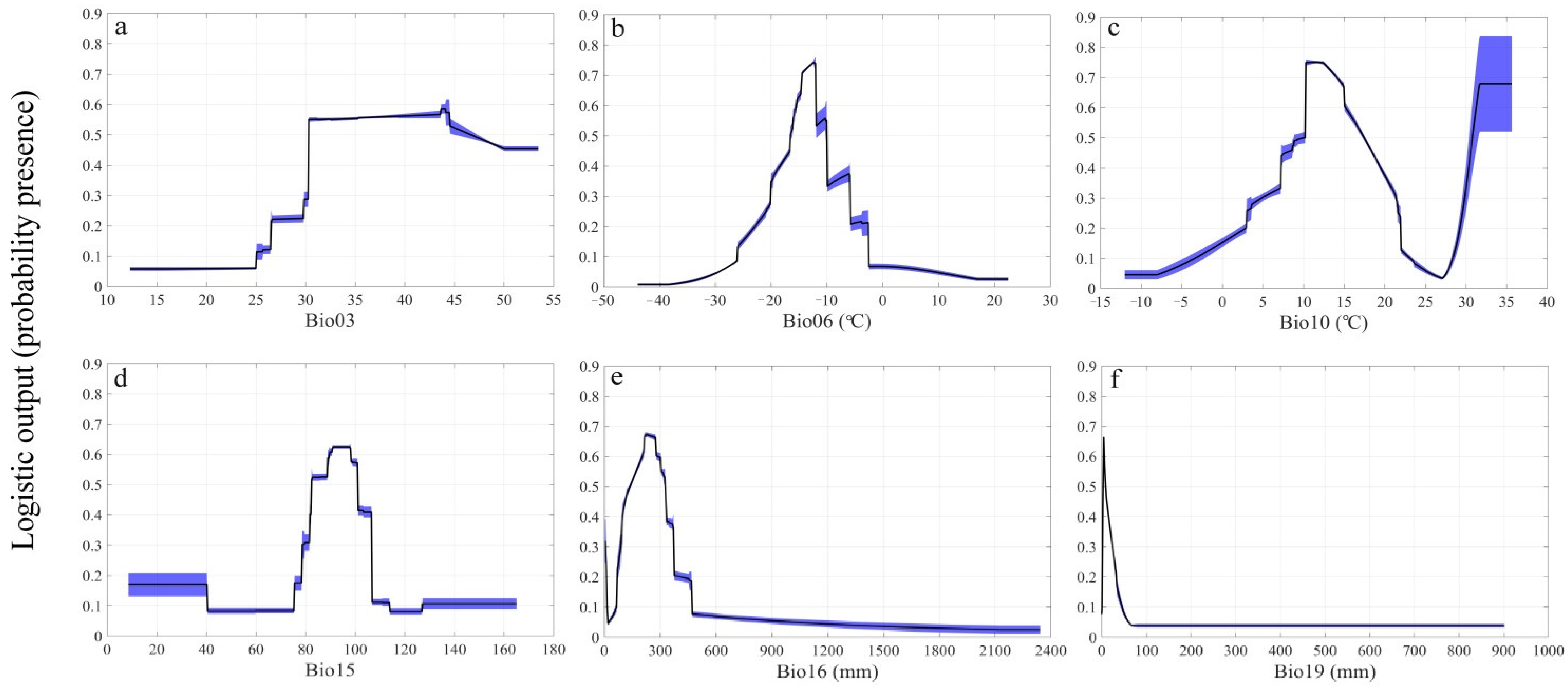
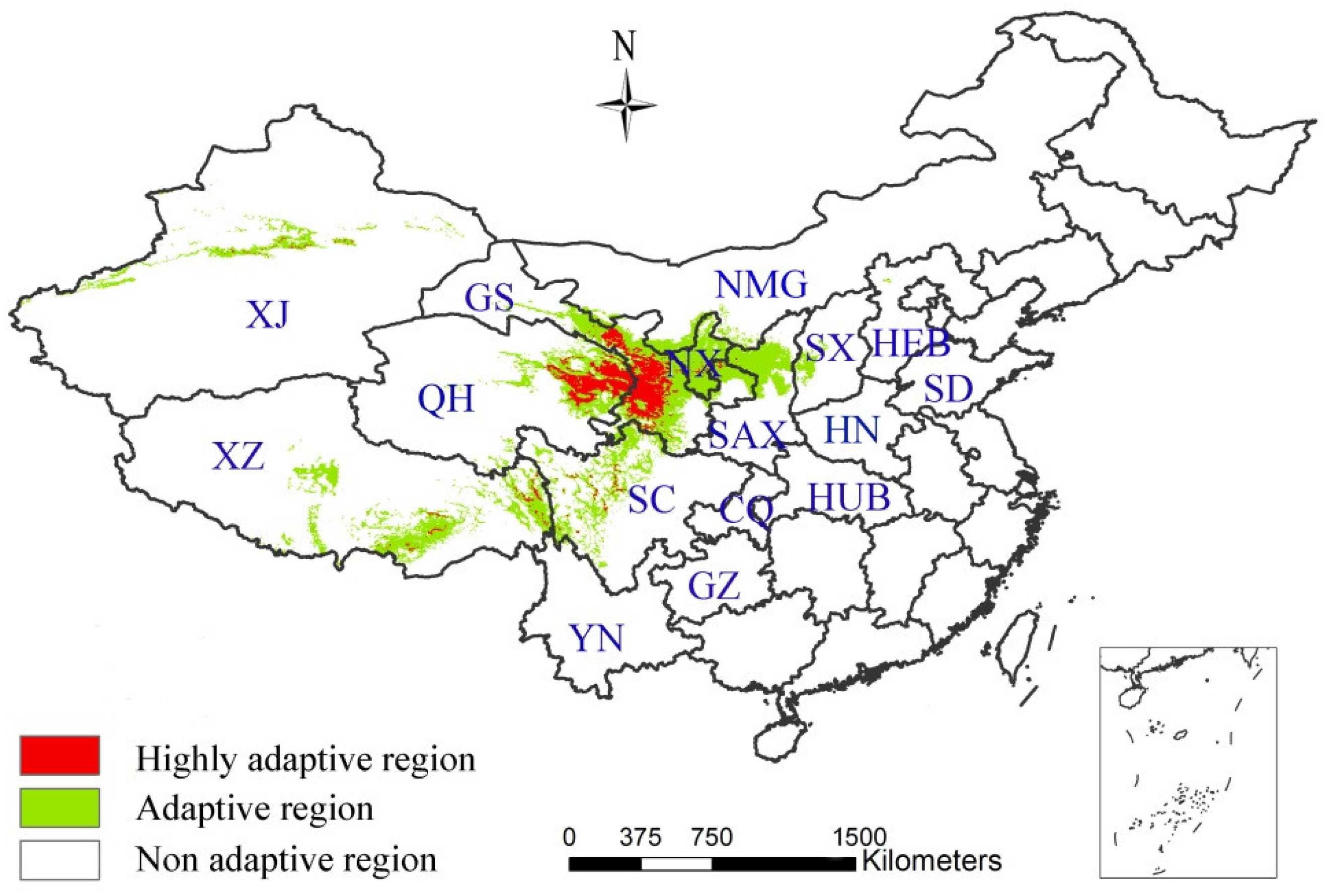
3.1. Model Performance and Importance of Predictor Variables

The contributions of seven environmental variables: Bio02, Bio03, Bio06, Bio10, Bio15 Bio16, and Bio19 were 1%, 9.5%, 15.1%, 17.4%, 14.5%, 16.9%, and 25.6%, respectively. By removing Bio02, the Maxent model of A. inebrians had a higher predictive power, such that the AUC = 0.91 ± 0.05 (mean ± SD) was increased by 0.01. When re-analyzed the contributions of the six environmental variables of Bio03, Bio06, Bio10, Bio15 Bio16, and Bio19 were 5.5%, 15.1%, 16.2%, 13.5%, 16.8%, and 25.9%.

The potential distribution probability of suitable habitats for A. inebrians can be maintained at a high level, the range of which varies slightly between 0.53 and 0.59, when the isothermality is between 30 and 45 (Figure 1a). In addition, the potential distribution probability exhibits a hump curve with increased temperature and precipitation (Figure 1b–f). When the minimum temperature of the coldest month equaled 12.05 °C the potential distribution probability reached its peak value (Figure 1b). The response curves also show that the suitable precipitation seasonality range is between 90.9 and 98.1, and that the potential distribution probability of A. inebrians exceeds 0.6 (Figure 1d). Similarly, the potential distribution probability rapidly reaches 0.6 when the precipitation of the wettest quarter increases to 218 mm, then rapidly decreases once the precipitation of the wettest quarter exceeds 300 mm (Figure 1e). The potential distribution probability is higher with a lower volume of precipitation during the coldest quarter (Figure 1f).

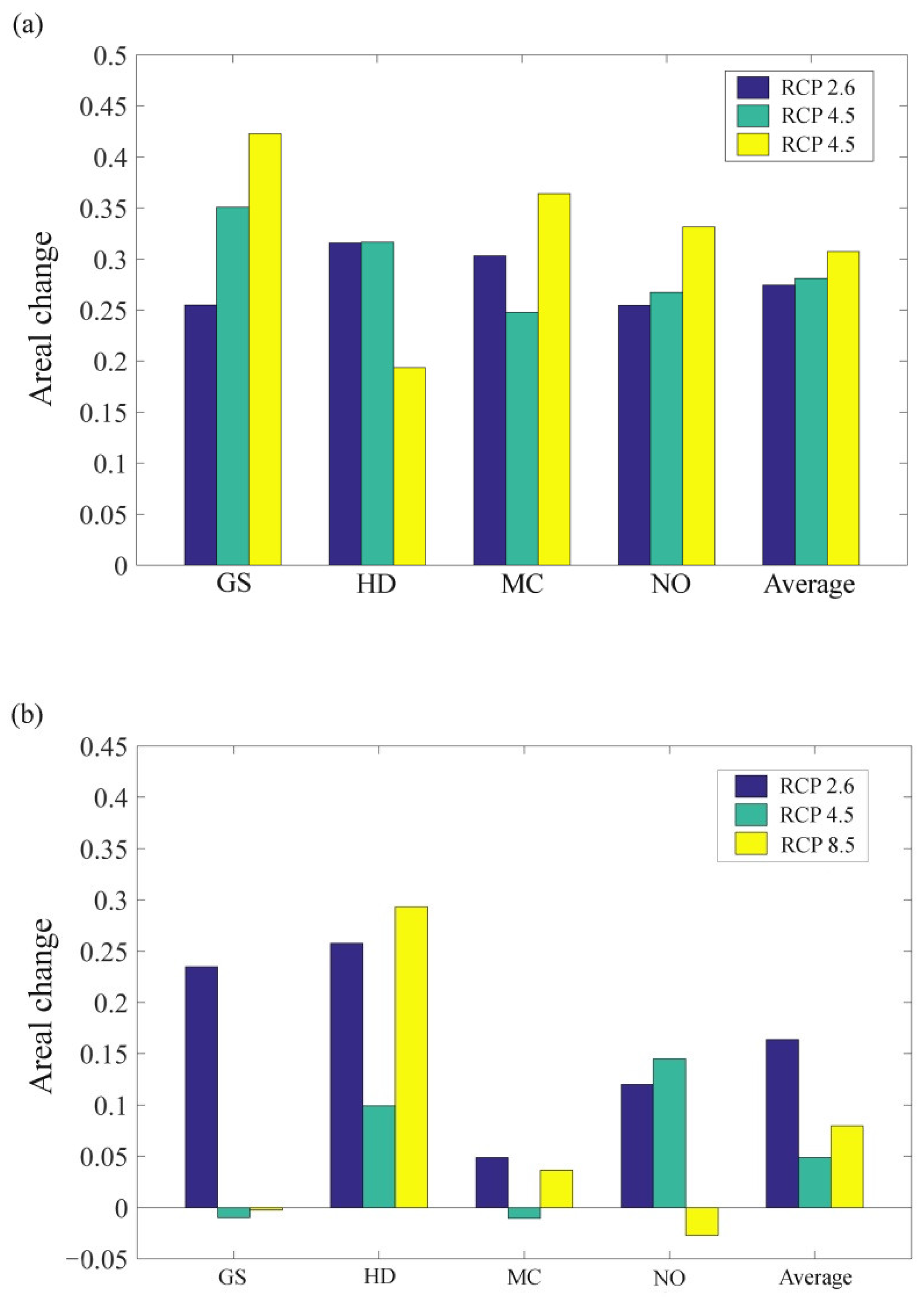
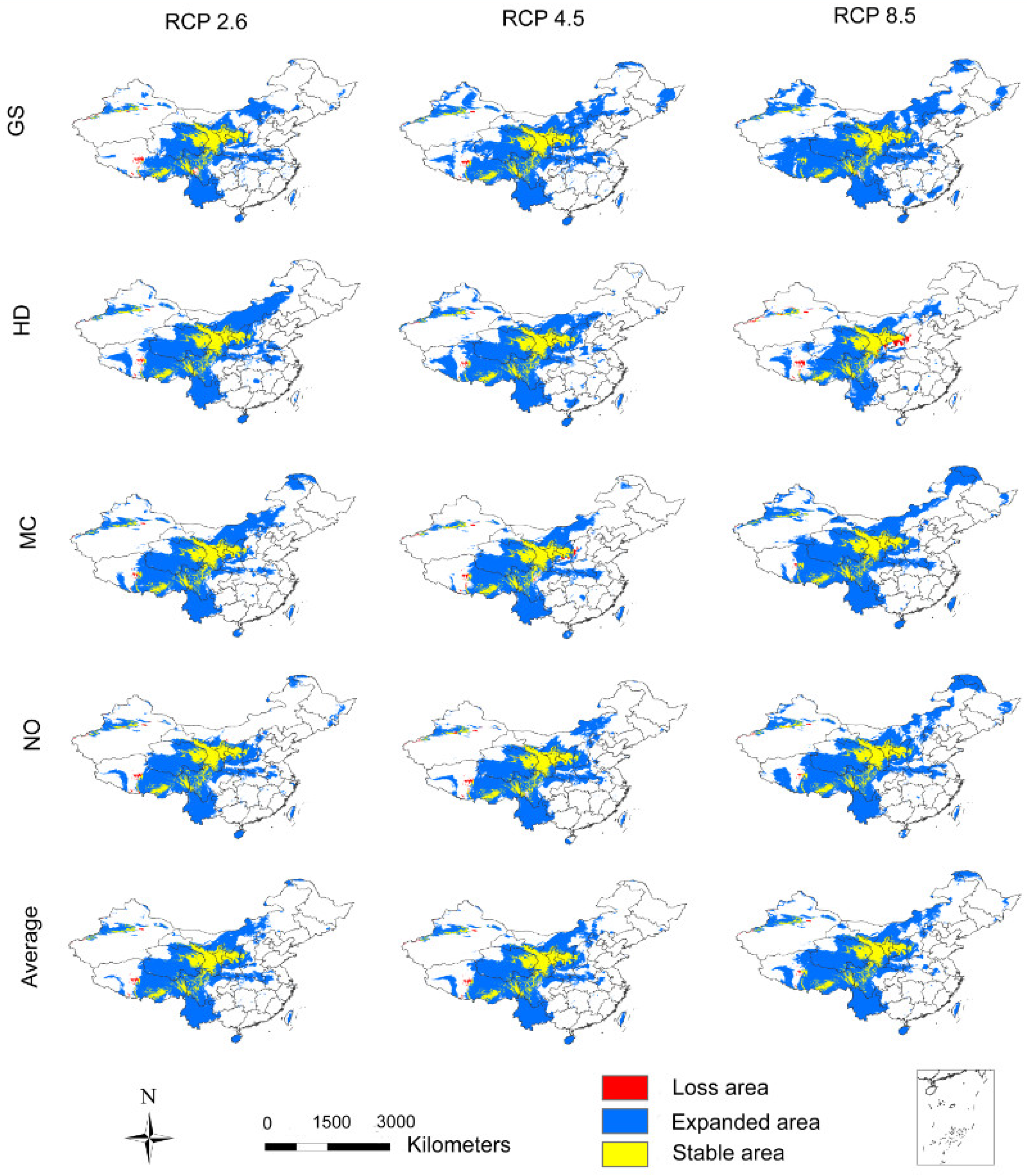
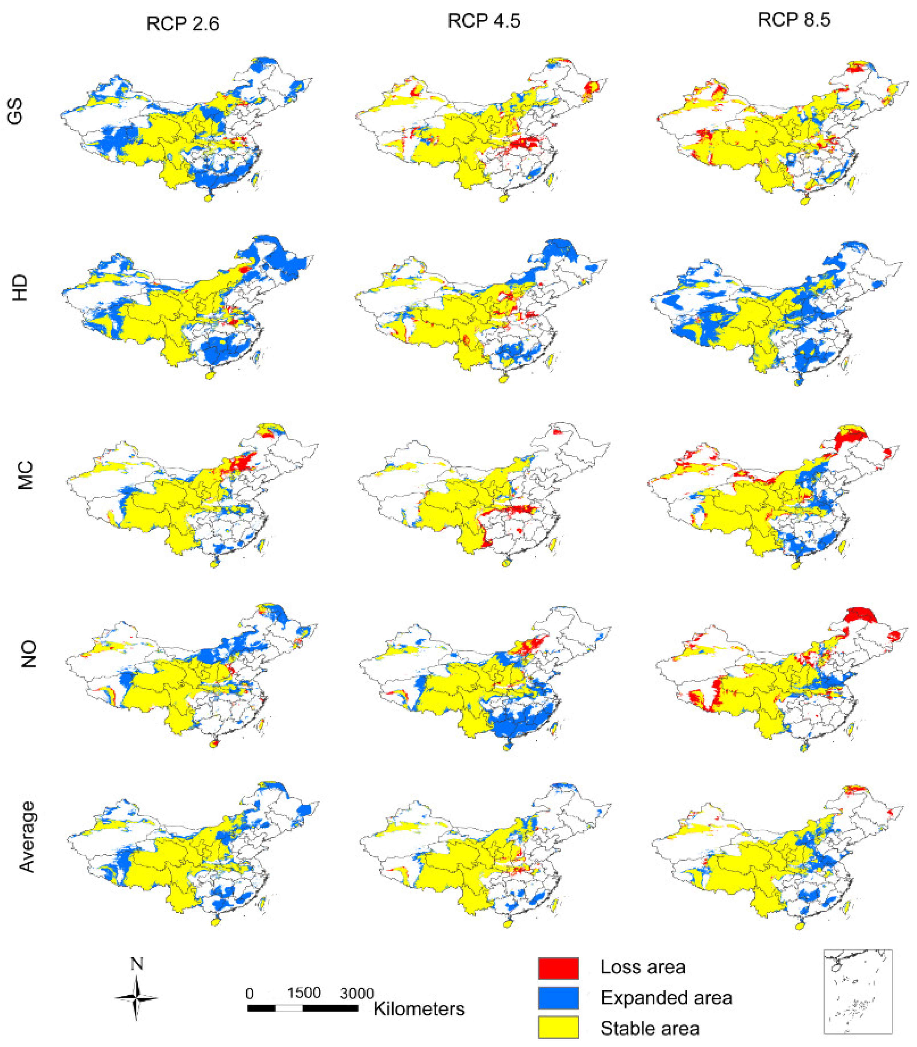
3.2. The Influence of CO₂ Emission Scenarios on the Potential Future Distributions of A. inebrians

The potential distributions of A. inebrians under current climatic conditions are classified according to the threshold value of 0.37 (Figure 2). The highly adaptive regions are mainly concentrated in the southwest of Gansu and east of Qinghai, while the adaptive regions are mainly distributed in the southeast of Gansu, Ningxia and north of Shaanxi. Both regions are considered typical temperate grasslands. In addition, the alpine meadow areas are scattered with a number of adaptive regions, such as Western Sichuan, Eastern Tibet and sporadic adaptation zones in Xinjiang.

CO₂ emission scenarios will continue to promote the gradual expansion of adaptive regions of A. inebrians into the future. In 2050, the adaptive region is projected to have expanded southwest (i.e., into the alpine meadow area) and northeast (i.e., into the temperate grassland area) with southern Gansu as its center (Figure 3). In the GS and NO models, the expansion characteristics of the adaptive regions are similar, in that as CO₂ emission scenarios increase, the area of the adaptive region grows, although the range of the adaptive region is larger in the GS model (Figure 3 and Figure 5a). However, the HD model predicts the exact opposite, indicating that low CO₂ emission scenarios are more suitable for the growth of A. inebrians (Figure 3 and Figure 5a). The MC model reveals that the adaptive region under high CO₂ emission scenarios is larger than with low CO₂ emission scenarios, but the adaptive region under medium CO₂ emission scenarios is the smallest of all the three (Figure 3 and Figure 5a). In summary, the average results indicate that higher CO₂ emission scenarios will cause a wider distribution of the adaptive region of A. inebrians by 2050.

After 2050, most of the adaptive regions of A. inebrians are stable. With low CO₂ emission scenarios, the adaptive regions are expanding, while they retract with high CO₂ emission scenarios in all models with the exception of HD. The average results also show that the area of the adaptive regions will have a greater expansion under low CO₂ emission scenarios than under high CO₂ emission scenarios after 2050 (Figure 4). With the exception of HD, the average data forecast after 2050 shows that the low CO₂ emission scenarios are more conducive to the survival of A. inebrians (Figure 5b).

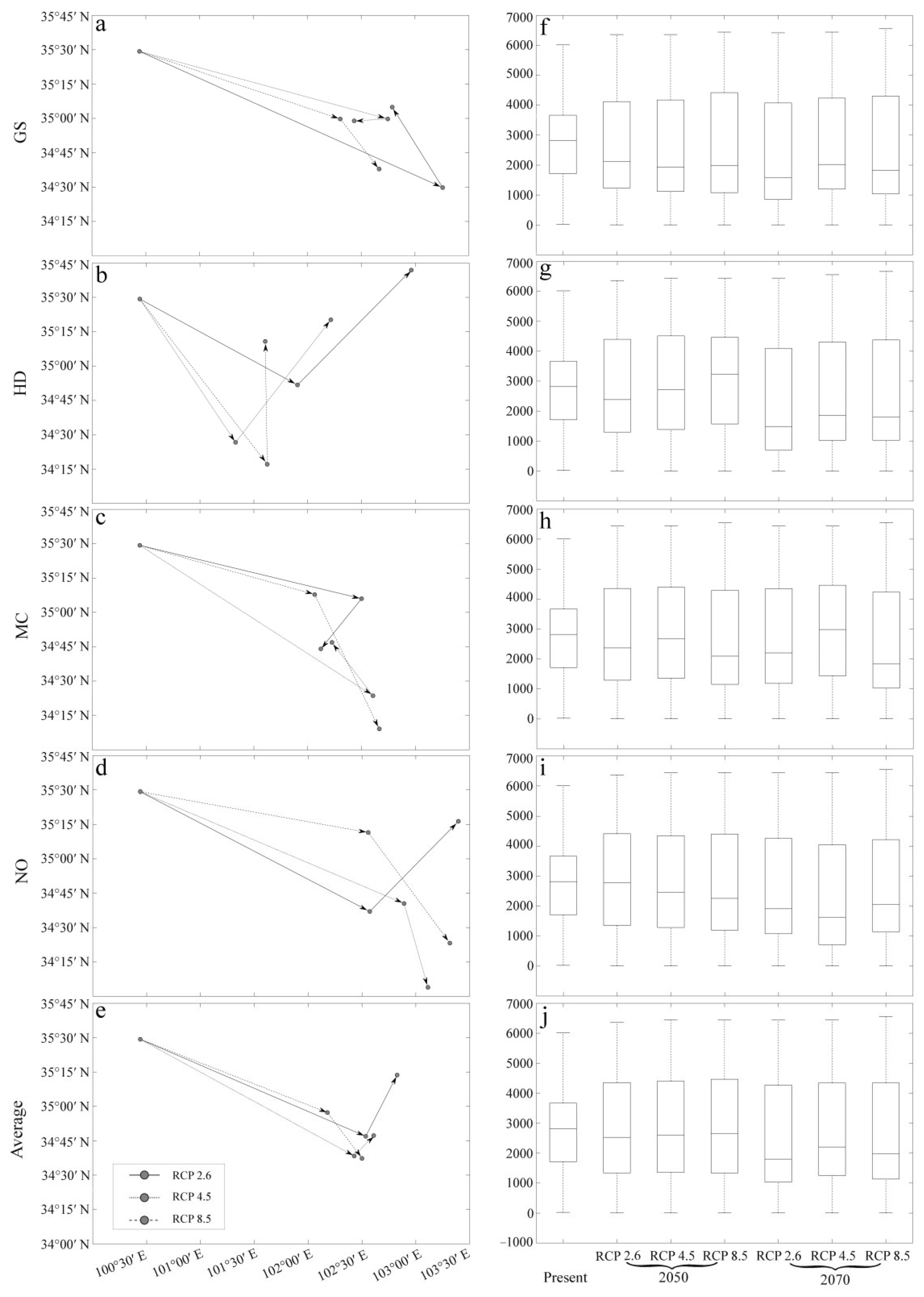
3.3. The Influence of CO₂ Emission Scenarios on the Geographical Distribution Centroid and Average Elevation of the Adaptive Regions of A. inebrians

From current conditions through to 2050, climate changes under the influence of CO₂ emission scenarios will likely cause the geographical distribution centroid of A. inebrians to move southeast, with a decrease in its latitude (Figure 6a–e). The GS and NO models predict that low CO₂ emission scenarios result in a latitudinal decrease in the geographical distribution centroid, whereas HD and MC models predict an increase (Figure 6a–d). The average results show that medium CO₂ emission scenarios also result in a latitudinal decrease in the geographical distribution centroid (Figure 6e). However, after 2050, the situation has reversed. With the exception of the MC models, the three others all project that low CO₂ emission scenarios can increase the latitude of the geographical distribution centroid, while high CO₂ emission scenarios result in a decrease (Figure 6a–e).

The average elevation of the adaptive regions of A. inebrians under the influence of CO₂ emission scenarios has a general downward trend. Low CO₂ emission scenarios continually decrease the average altitude, but the medium and high CO₂ emissions only reveal a trend of lowering the average elevation after 2050 (Figure 6f–i). The average results show that the average elevation of the adaptive regions’ decline slows with the increase in CO₂ emission scenarios (Figure 6j).

4. Discussions

Carbon dioxide (CO₂) is the most important greenhouse gas released as a result of anthropogenic activity. This study has modelled the effect of three different CO₂ emission scenarios (RCP 2.6, 4.5, and 8.5) on the potential future distributions of A. inebrians. The response of the Maxent results to the environmental variables indicates that in the coldest month/quarter, which is also the dormant period of seeds of A. inebrians, the potential distribution probability of A. inebrians is higher when the minimum temperature and precipitation are lower. This is likely because the seed germination rate of weeds is higher after dormancy in lower temperatures [51,52,53]. Moreover, light drought stress is more conducive to the embryonic root growth of A. inebrians [54]. During the growing season, moderate temperature and rainfall are clearly beneficial to the growth of weeds; hence the ecological niche model also includes two other important factors: the mean temperature of the warmest quarter and the precipitation of the wettest quarter. The increase in CO₂ emission concentration has had a significant impact on increasing temperatures in most areas of China, especially in the northwest [55]. In addition, it has influenced the precipitation patterns, with Northwest China becoming even drier and the coastal areas more humid [56]. Furthermore, with increases in CO₂ emission concentration, seasonal fluctuations of extreme climates are likely to occur more frequently and with larger amplitudes [15,57].

It is predicted that the suitable regions for A. inebrians in 2050 will greatly expand, extending to the Inner Mongolia grassland and the Qinghai–Tibet Plateau, while the expansion range is relatively smaller from 2050 to 2070. Our research supports the conclusions of Saebø and Mortensen (1998) and Singh et al. (2011) that increasing CO₂ emission scenarios are beneficial to the growth of perennial herbs [23,24]. However, the reason for the expansion of suitable habitats for A. inebrians after 2050 is not clear. It is possible that after 2050, in addition to RCP 8.5, the CO₂ emission concentration of other scenarios may be alleviated, especially with the CO₂ emission concentration of RCP 2.6 beginning to decline. Additionally, the two time periods we studied were different in length, 50 years and 20 years, respectively. Our research also identified that various intensities of CO₂ emissions induce extremely different effects on the expansion of A. inebrians. Most GCM (except HD) simulations show that the high CO₂ emission scenarios model increase range expansion before 2050; while after 2050, the low CO₂ emissions scenarios model results in range expansion. The average results not only draw the same conclusions, but also reveal that the scope of expansion increases with the increase in CO₂ emission scenarios before 2050. Our findings are different compared to Dyderski et al. (2018) and Wróblewska & Mirski (2018), as different species have different niches and naturally respond differently to climate change [16,17]. Unlike tree species and circumboreal plants, CO₂ may have a positive effect on the growth and reproduction of A. inebrians.

Under anthropogenically induced climate change, migration and diffusion have become a significant response mechanism for plants. Many species will disperse to areas with the most suitable climate for their growth to maintain homeostasis. Some studies have found that global warming led to a poleward and upward shift in the range of many plants [13,58,59], but not all plants, as some engaged in southerly migration [60]. The geographical distribution centroids of A. inebrians were generally projected to move southeast under different CO₂ emission scenarios. However, the direction of the geographical distribution centroids will likely be diversified after 2050, especially under low CO₂ emission scenarios with a latitudinal recovery of the geographical distribution centroids. With the increase in CO₂ concentration, there was a predicted decline in the average elevation of the potential distributions. In all GCM models, we identified that the changes in the geographical distribution centroids and average elevation predicted by the HD model were significantly different from the other three. The HD results show that the latitude of the geographical distribution centroids under the low emission scenarios in 2070 was higher than that of the current latitude, and even that under the high CO₂ emission scenarios in 2050. This result seems to support the conclusion that plants migrate to higher altitudes and higher latitudes in future climate change scenarios [13,58,59]. Therefore, the impact of CO₂ emission scenarios on the potential distribution of A. inebrians is strongly influenced by the choice of GCMs.

The uncertainty of future climates is one of the critical issues in accurately predicting the effects of climate change. It is therefore one of the core issues that needs to be addressed for conservation planning of livestock management [10,61]. In this study, four GCMs were used to explore the effect of climate uncertainty caused by different GCMs on the potential distribution areas of A. inebrians, respectively. We did not directly adopt the ensembles of the GCMs as in previous studies [48] but used the average of the results predicted under four GCMs. The average results not only mitigate the effects of future climate uncertainties by GCMs, but also preserve the impact of the spatial pattern of each GCM on the final results. Furthermore, three RCPs were also used to explore the impact of climate uncertainty caused by different CO₂ emissions on the potential distribution areas of A. inebrians. It has been reported that the maximum possibility of CO₂ emission scenarios in China is RCP4.5 in the future [62]. Our average results under RCP4.5 indicate that the adaptive regions of A. inebrians in 2050 are significantly greater than currently observed, mainly distributed in central Inner Mongolia, southern Gansu, Ningxia, eastern Inner Mongolia, Yunnan, most parts of Qinghai, Shaanxi, and Sichuan. However, the changes in the adaptive regions are not significantly different in 2070, with only small plaque growth in Southeast China and sporadic reductions in Shaanxi.

Samples and environmental variables are two important factors in ecological niche modeling, while sample bias and different strategies for selecting environmental variables can also seriously influence the results of ecological niche modeling [63,64,65]. In our study, the sample bias was reduced by utilizing the nearest neighbor method (i.e., randomly removing one of the two points below the minimum neighbor distance) [66]. At the same time, principal component analysis and correlation analysis were used to select the environmental variables used. Based on the processing of samples and rational selection of environmental variables, the ecological niche model obtained good prediction results, which reinforces the reliability of our results. Moreover, it is important to note that the above estimation of the potential distribution regions of A. inebrians was only based on Maxent. However, the ENM alone is not successful at predicting the eventual spread of a species [67], many factors other than climate, such as population processes, biotic interactions, dispersal ability, interactions between demographic, and landscape dynamics, also play an important part in determining species distributions [68,69]. Furthermore, land use patterns may play an important role in predicting the potential distributions [70]. Therefore, a comprehensive model combined with all the above mentioned factors is necessary for the prediction of species-specific responses to climate change and useful agricultural suggestions to the managers and administrators.

References

1. Houghton, J.T.; Filho, L.G.M.; Callander, B.A.; Harris, N.; Kattenburg, A.; Maskell, K. Climate Change 1995: The Science of Climate Change; Cambridge University Press: Cambridge, UK, 1996; p. 584. [Google Scholar]
2. Shahbaz, M.; Shahzad, S.J.H.; Mahalik, M.K. Is globalization detrimental to CO2 emissions in Japan? New threshold analysis. Environ. Model. Assess. 2017, 23, 557–568. [Google Scholar] [CrossRef] [Green Version]
3. Folland, C.K.; Boucher, O.; Colman, A.; Parker, D.E. Causes of irregularities in trends of global mean surfacetemperature since the late 19th century. Sci. Adv. 2018, 4, 5297. [Google Scholar] [CrossRef] [PubMed] [Green Version]
4. Van Mai, T.; Lovell, J. Impact of climate change, adaptation and potential mitigation to Vietnam agriculture. In Handbook of Climate Change Mitigation and Adaptation; Chen, W.-Y., Suzuki, T., Lackner, M., Eds.; Springer: New York, NY, USA, 2016; pp. 1–26. [Google Scholar]
5. Bajwa, A.A.; Wang, H.; Chauhan, B.S.; Adkins, S.W. Effect of elevated carbon dioxide concentration on growth, productivity and glyphosate response of parthenium weed (Parthenium hysterophorus L.). Pest Manag. Sci. 2019, 75, 2934–2941. [Google Scholar] [CrossRef] [PubMed]
6. IPPC. Climate Change 2013: The Physical Science Basis. Contribution of Working Group I to the Fifth Assessment Report of the Intergovernmental Panel on Climate Change; Cambridge University Press: Cambridge, UK; New York, NY, USA, 2013. [Google Scholar]
7. Harris, R.M.B.; Grose, M.R.; Lee, G.; Bindoff, N.L.; Porfirio, L.L.; Fox-Hughes, P. Climate projections for ecologists. WIREs Clim. Change 2014, 5, 621–637. [Google Scholar] [CrossRef]
8. Meinshausen, M.; Smith, S.J.; Calvin, K.; Daniel, J.S.; Kainuma, M.L.T.; Lamarque, J.-F.; Matsumoto, K.; Montzka, S.A.; Raper, S.C.B.; Riahi, K.; et al. The RCP greenhouse gas concentrations and their extensions from 1765 to 2300. Clim. Change 2011, 109, 213–241. [Google Scholar] [CrossRef] [Green Version]
9. van Vuuren, D.P.; Edmonds, J.; Kainuma, M.; Riahi, K.; Thomson, A.; Hibbard, K.; Hurtt, G.C.; Kram, T.; Krey, V.; Lamarque, J.-F.; et al. The representative concentration pathways: An overview. Clim. Change 2011, 109, 5–31. [Google Scholar] [CrossRef]
10. Koo, K.A.; Park, S.U.; Kong, W.-S.; Hong, S.; Jang, I.; Seo, C. Potential climate change effects on tree distributions in the Korean Peninsula: Understanding model & climate uncertainties. Ecol. Model. 2017, 353, 17–27. [Google Scholar]
11. Ernakovich, J.G.; Hopping, K.A.; Berdanier, A.B.; Simpson, R.T.; Kachergis, E.J.; Steltzer, H.; Wallenstein, M.D. Predicted responses of arctic and alpine ecosystems to altered seasonality under climate change. Glob. Change Biol. 2014, 20, 3256–3269. [Google Scholar] [CrossRef]
12. Flagmeier, M.; Long, D.G.; Genney, D.R.; Hollingsworth, P.M.; Ross, L.C.; Woodin, S.J. Fifty years of vegetation change in oceanic-montane liverwort-rich heath in Scotland. Plant Ecol. Divers. 2014, 7, 457–470. [Google Scholar] [CrossRef]
13. Pauli, H.; Gottfried, M.; Dullinger, S.; Abdaladze, O.; Akhalkatsi, M.; Alonso, J.L.B.; Coldea, G.; Dick, J.; Erschbamer, B.; Calzado, R.F.; et al. Recent plant diversity changes on Europe’s mountain summits. Science 2012, 336, 353–355. [Google Scholar] [CrossRef] [Green Version]
14. Sproull, G.J.; Quigley, M.F.; Sher, A.; González, E. Long-term changes in composition, diversity and distribution patterns in four herbaceous plant communities along an elevational gradient. J. Veg. Sci. 2015, 26, 552–563. [Google Scholar] [CrossRef]
15. Walther, G.; Post, E.; Convey, P.; Menzel, A.; Parmesan, C.; Beebee, T.; Fromentin, J.; Hoegh-Guldberg, O.; Bairlein, F. Ecological responses to recent climate change. Nature 2002, 416, 389–395. [Google Scholar] [CrossRef] [PubMed]
16. Dyderski, M.K.; Paź, S.; Frelich, L.E.; Jagodziński, A.M. How much does climate change threaten European forest tree species distributions? Glob. Change Biol. 2018, 24, 1150–1163. [Google Scholar] [CrossRef] [PubMed]
17. Wróblewska, A.; Mirski, P. From past to future: Impact of climate change on range shifts and genetic diversity patterns of circumboreal plants. Reg. Environ. Change 2018, 18, 409–424. [Google Scholar] [CrossRef] [Green Version]
18. Peters, K.; Breitsameter, L.; Gerowitt, B. Impact of climate change on weeds in agriculture: A review. Agron. Sustain. Dev. 2014, 34, 707–721. [Google Scholar] [CrossRef] [Green Version]
19. Patterson, D.T. Weeds in a changing climate. Weed Sci. 1995, 43, 685–700. [Google Scholar] [CrossRef]
20. McDonald, A.; Riha, S.; DiTommaso, A.; DeGaetano, A. Climate change and the geography of weed damage: Analysis of U.S. maize systems suggests the potential for significant range transformations. Agric. Ecosyst. Environ. 2009, 130, 131–140. [Google Scholar] [CrossRef]
21. Ziska, L.H.; Goins, E.W. Elevated atmospheric carbon dioxide and weed populations in glyphosate treated soybean. Crop Sci. 2006, 46, 1354–1359. [Google Scholar] [CrossRef]
22. Jabran, K.; Dogan, M.N. High carbon dioxide concentration and elevated temperature impact the growth of weeds but do not change the efficacy of glyphosate. Pest Manag. Sci. 2018, 74, 766–771. [Google Scholar] [CrossRef]
23. Saebø, A.; Mortensen, L. Influence of elevated atmospheric CO2 concentration on common weeds in Scandinavian agriculture. Acta Agric. Scand. 1998, 48, 138–143. [Google Scholar]
24. Singh, R.P.; Singh, R.K.; Singh, M.K. Impact of climate and carbon dioxide change on weeds and their management-a Review. Indian J. Weed Sci. 2011, 43, 1–11. [Google Scholar]
25. Williams, A.L.; Wills, K.E.; Janes, J.K.; Schoor, J.K.V.; Newton, P.C.D.; Hovenden, M.J. Warming and free-air CO2 enrichment alter demographics in four co-occurring grassland species. New Phytol. 2007, 176, 365–374. [Google Scholar] [CrossRef] [PubMed]
26. Chen, L.; Li, X.Z.; Li, C.J.; Swoboda, G.A.; Schardl, C.L. Two distinct Epichloë species symbiotic with Achnatherum inebrians, drunken horse grass. Mycologia 2015, 107, 863–873. [Google Scholar] [CrossRef] [PubMed] [Green Version]
27. Huoman, S. Achnatherum Inebrians and its prevented and cured measures. Pratacult. Sci. 1992, 9, 36–37. [Google Scholar]
28. Li, C.-J.; Gao, J.-H.; Ma, B. Seven diseases of drunken horse grass (Achnatherum inebrians) in China. Pratacult. Sci. 2003, 21, 51–53. [Google Scholar]
29. Shi, Z. Important Poisonous Plants of China Grassland; China Agricultural Press: Beijing, China, 1997. [Google Scholar]
30. Li, X.; Ren, J.; Feng, K.; Lei, T.; Ar, Y.; Zhang, X. Ecological control method of Achnatherum inebrians. Pratacult. Sci. 1996, 5, 14–17. [Google Scholar]
31. Vilà, M.; Beaury, E.M.; Blumenthal, D.M.; Bradley, B.A.; Ibanez, I. Understanding the combined impacts of weeds and climate change on crops. Environ. Res. Lett. 2021, 16, 034043. [Google Scholar] [CrossRef]
32. Albright, T.P.; Chen, H.; Chen, L.; Guo, Q. The ecological niche and reciprocal prediction of the disjunct distribution of an invasive species: The example of Ailanthus altissima. Biol. Invasions 2010, 12, 2413–2427. [Google Scholar] [CrossRef]
33. Medley, K.A. Niche shifts during the global invasion of the Asian tiger mosquito, Aedes albopictus Skuse (Culicidae), revealed by reciprocal distribution models. Glob. Ecol. Biogeogr. 2010, 19, 122–133. [Google Scholar] [CrossRef]
34. Peterson, A.T. Predicting the geography of species’ invasions via ecological niche modeling. Q. Rev. Biol. 2003, 78, 419–433. [Google Scholar] [CrossRef] [Green Version]
35. Olivera, L.; Minghetti, E.; Montemayor, S.I. Ecological niche modeling (ENM) of Leptoglossus clypealis a new potential global invader: Following in the footsteps of Leptoglossus occidentalis? Bull. Entomol. Res. 2021, 111, 289–300. [Google Scholar] [CrossRef] [PubMed]
36. Fuchs, A.J.; Gilbert, C.C.; Kamilar, J.M. Ecological niche modeling of the genus Papio. Am. J. Phys. Anthropol. 2018, 166, 812–823. [Google Scholar] [CrossRef] [PubMed] [Green Version]
37. Kolanowska, M.; Rewicz, A.; Baranow, P. Ecological niche modeling of the pantropical orchid Polystachya concreta (Orchidaceae) and its response to climate change. Sci. Rep. 2020, 10, 14801. [Google Scholar] [CrossRef] [PubMed]
38. Pearson, R.G. Species’ distribution modeling for conservation educators and practitioners. Lesson Conserv. 2010, 3, 54–89. [Google Scholar]
39. Zhu, G.; Liu, G.; Bu, W.; Gao, Y. Ecological niche modeling and its applications in biodiversity conservation. Biodivers. Sci. 2013, 21, 90–98. [Google Scholar]
40. Phillips, S.J.; Anderson, R.P.; Schapire, R.E. Maximum entropy modeling of species geographic distributions. Ecol. Model. 2006, 190, 231–259. [Google Scholar] [CrossRef] [Green Version]
41. Sun, X.; Xu, Q.; Luo, Y. A maximum entropy model predicts the potential geographic distribution of Sirex noctilio. Forests 2020, 11, 175. [Google Scholar] [CrossRef] [Green Version]
42. Gibson, L.; Barrett, B.; Burbidge, A. Dealing with uncertain absences in habitat modelling: A case study of a rare ground-dwelling parrot. Divers. Distrib. 2007, 13, 704–713. [Google Scholar] [CrossRef]
43. Peterson, A.T.; Pape, M.; Eaton, M. Transferability and model evaluation in ecological niche modeling: A comparison of GARP and Maxent. Ecography 2007, 30, 550–560. [Google Scholar] [CrossRef]
44. Wisz, M.S.; Hijmans, R.J.; Li, J.; Peterson, A.T.; Graham, C.H.; Guisan, A. Effects of sample size on the performance of species distribution models. Divers. Distrib. 2008, 14, 763–773. [Google Scholar] [CrossRef]
45. Radosavljevic, A.; Anderson, R.P. Making better Maxent models of species distributions: Complexity, overfitting and evaluation. J. Biogeogr. 2014, 41, 629–643. [Google Scholar] [CrossRef]
46. Bagchi, R.; Crosby, M.; Huntley, B.; Hole, D.G.; Butchart, S.H.M.; Collingham, Y.; Kalra, M.; Rajkumar, J.; Rahmani, A.; Pandey, M.; et al. Evaluating the effectiveness of conservation site networks under climate change: Accounting for uncertainty. Glob. Change Biol. 2013, 19, 1236–1248. [Google Scholar] [CrossRef] [PubMed] [Green Version]
47. Thuiller, W. Patterns and uncertainties of species’ range shifts under climate change. Glob. Change Biol. 2004, 10, 2020–2027. [Google Scholar] [CrossRef]
48. Baker, D.J.; Hartley, A.J.; Butchart, S.H.; Willis, S.G. Choice of baseline climate data impacts projected species’ responses to climate change. Glob. Change Biol. 2016, 22, 2392–2404. [Google Scholar] [CrossRef] [Green Version]
49. Wang, T.; Wang, G.; Innes, J.; Nitschke, C.; Kang, H. Climatic niche models and their consensus projections for future climates for four major forest tree species in the Asia–Pacific region. For. Ecol. Manag. 2016, 360, 357–366. [Google Scholar] [CrossRef]
50. Hortal, J.; Jiménez-Valverde, A.; Gómez, J.F.; Lobo, J.M.; Baselga, A.J.O. Historical bias in biodiversity inventories affects the observed environmental niche of the species. Oikos 2010, 117, 847–858. [Google Scholar] [CrossRef]
51. Kang, B.H.; Shim, S.I.; Lee, S.G.; Shin, H.W. Physiological and ecological studies on the seed dormancy of dominant weed species in Korea. Korean J. Environ. Agric. 1993, 12, 193–207. [Google Scholar]
52. Guan, X.; Ramaswamy, H.; Zhang, B.; Lin, B.; Wang, S. Influence of moisture content, temperature and heating rate on germination rate of watermelon seeds. Sci. Hortic. 2020, 272, 109528. [Google Scholar] [CrossRef]
53. Tian, Z.-H.; Shen, G.-H. Advance on regulation of seed dormancy and germination of weeds. Acta Agric. Shanghai 2015, 31, 137–141. [Google Scholar]
54. Yu, X.-J.; Chen, B.-J.; Shi, S.-L.; Wei, G.-B.; Man, Y.-R.; Ma, Y.-L. Effect of temperature and moisture condition on seed germination of Achnatherum Inebriants (Hance) Keng. Acta Agrestia Sin. 2009, 17, 218–221. [Google Scholar]
55. Cowie, B.W.; Venter, N.; Witkowski, E.; Byrne, M.J. Implications of elevated carbon dioxide on the susceptibility of the globally invasive weed, parthenium hysterophorus, to glyphosate herbicide. Pest Manag. Sci. 2020, 76, 2324–2332. [Google Scholar] [CrossRef] [PubMed]
56. Zhang, Q.; Zhu, Y.; Li, Y.; Ni, Y. Effects of atmospheric CO2 doubling on the climate. Sci. Meteorol. Sin. 1994, 14, 16–22. [Google Scholar]
57. Jentsch, A.; Kreyling, J.; Boettcher-Treschkow, J.; Beierkuhnlein, C. Beyond gradual warming: Extreme weather events alter flower phenology of European grassland and heath species. Glob. Change Biol. 2009, 15, 837–849. [Google Scholar] [CrossRef]
58. Chen, I.C.; Hill, J.K.; Ohlemuller, R.; Roy, D.B.; Thomas, C.D. Rapid Range Shifts of Species Associated with High Levels of Climate Warming. Science 2011, 333, 1024–1026. [Google Scholar] [CrossRef] [PubMed]
59. Li, M.H.; Kräuchi, N.; Gao, S.P. Global warming: Can existing reserves really preserve current levels of biological diversity? J. Integr. Plant Biol. 2006, 48, 255–259. [Google Scholar] [CrossRef]
60. Midgley, G.F.; Hannah, L.; Millar, D.; Thuiller, W.; Booth, A. Developing regional and species-level assessments of climate change impacts on biodiversity in the Cape Floristic Region. Biol. Conserv. 2003, 112, 87–97. [Google Scholar] [CrossRef]
61. Wang, T.; Campbell, E.M.; O’Neill, G.A.; Aitken, S.N. Projecting future distributions of ecosystem climate niches: Uncertainties and management applications. For. Ecol. Manag. 2012, 279, 128–140. [Google Scholar] [CrossRef]
62. Chen, M.; Lin, E. Global greenhouse gas emission mitigation under representative concentration pathways scenarios and challenges to China. Adv. Clim. Change Res. 2010, 80, 436–442. [Google Scholar]
63. Baselga, A.; Araújo, M. Individualistic vs. community modelling of species distributions under climate change. Ecography 2010, 32, 55–65. [Google Scholar] [CrossRef]
64. Phillips, S.J.; Miroslav, D.; Jane, E.; Graham, C.H.; Anthony, L.; John, L.; Simon, F. Sample selection bias and presence-only distribution models: Implications for background and pseudo-absence data. Ecol. Appl. 2009, 19, 181–197. [Google Scholar] [CrossRef] [Green Version]
65. Stockwell, D.R.B. Improving ecological niche models by data mining large environmental datasets for surrogate models. Ecol. Model. 2005, 192, 188–196. [Google Scholar] [CrossRef] [Green Version]
66. Levsen, N.D.; Tiffin, P.; Olson, M.S. Pleistocene speciation in the genus Populus (salicaceae). Syst. Biol. 2012, 61, 401–412. [Google Scholar] [CrossRef] [PubMed] [Green Version]
67. Sax, D.F.; Stachowicz, J.J.; Brown, J.H.; Bruno, J.F.; Dawson, M.N.; Gaines, S.D.; Grosberg, R.K.; Hastings, A.; Holt, R.D.; Mayfield, M.M. Ecological and evolutionary insights from species invasions. Trends Ecol. Evol. 2007, 22, 465–471. [Google Scholar] [CrossRef] [PubMed]
68. Keith, D.A.; HResit, A.A.; Wilfried, T.; Midgley, G.F.; Pearson, R.G.; Phillips, S.J.; Regan, H.M.; Araújo, M.B.; Rebelo, T.G. Predicting extinction risks under climate change: Coupling stochastic population models with dynamic bioclimatic habitat models. Biol. Lett. 2008, 4, 560–563. [Google Scholar] [CrossRef]
69. Pearson, R.G.; Dawson, T.P. Predicting the impacts of climate change on the distribution of species: Are bioclimate envelope models useful? Glob. Ecol. Biogeogr. 2003, 12, 361–371. [Google Scholar] [CrossRef] [Green Version]
70. Taylor, S.; Kumar, L.; Reid, N. Impacts of climate change and land-use on the potential distribution of an invasive weed: A case study of Lantana camara in Australia. Weed Res. 2012, 52, 391–401. [Google Scholar] [CrossRef]
Figure 1. Response curves display the relationships between the potential distribution probability of A. inebrians and six environmental variables, including (a) Isothermality (Bio03), (b) Min Temperature of Coldest Month (Bio06), (c) Mean Temperature of Warmest Quarter (Bio10), (d) Precipitation Seasonality (Bio15), (e) Precipitation of Wettest Quarter (Bio16), and (f) Precipitation of Coldest Quarter (Bio19). Values shown are the average over 20 replicate runs; blue margins show ± SD calculated over 20 replicates.
Sustainability 14 04806 g001
Figure 2. The potential distributions of A. inebrians under current climatic conditions.
Sustainability 14 04806 g002
Figure 3. The potential distribution changes of A. inebrians in 2050 in comparison to current trends. The first four rows are the results of four GCMs, i.e., GS, HD, MC, and NO. Additionally, the last row is the average of the results of four GCMs. The columns show results under three CO2 emission scenarios, i.e., RCP 2.6, 4.5, and 8.5.
Sustainability 14 04806 g003
Figure 4. The potential distribution changes of A. inebrians in 2070 in comparison to 2050. The first four rows are the results of four GCMs, i.e., GS, HD, MC, and NO. Additionally, the last row is the average of the results of four GCMs. The columns show results under three CO2 emission scenarios, i.e., RCP 2.6, 4.5, and 8.5.
Sustainability 14 04806 g004
Figure 5. The impact of three CO2 emission scenarios (RCP 2.6, 4.5, and 8.5) on the potential distribution changes of A. inebrians. (a) The changes of the potential distribution in 2050 compared to current trends; (b) the changes of the potential distribution in 2070 compared to 2050. GS, HD, MC, and NO are four GCMs, and average represents the average of the results of four GCMs.
Sustainability 14 04806 g005
Figure 6. The effect of three CO2 emission scenarios (RCP 2.6, 4.5, and 8.5) on the geographical distribution centroid and average elevation of the adaptive regions of A. inebrians. The first four rows are the results of four GCMs, i.e., GS, HD, MC, and NO. Additionally, the last row is the average of the results of four GCMs. (ae) Changes in the geographical distribution centroid of the adaptive regions of A. inebrians from present to future (2050 and 2070). The black dot is the geographical distribution centroid, and the arrow represents the direction of time change. (fj) Boxplots of elevation of the adaptive regions of A. inebrians under different climate scenarios.
Sustainability 14 04806 g006