
A Sustainable Supply Chain Network Model Considering Carbon Neutrality and Personalization


Abstract
:1. Introduction
2. Literature Review
2.1. Carbon Neutrality and Sustainable Supply Chain
2.2. Personalization and Sustainable Supply Chain
2.3. The Method of HD and GA
3. The SSCN Model
4. Mathematical Formulation
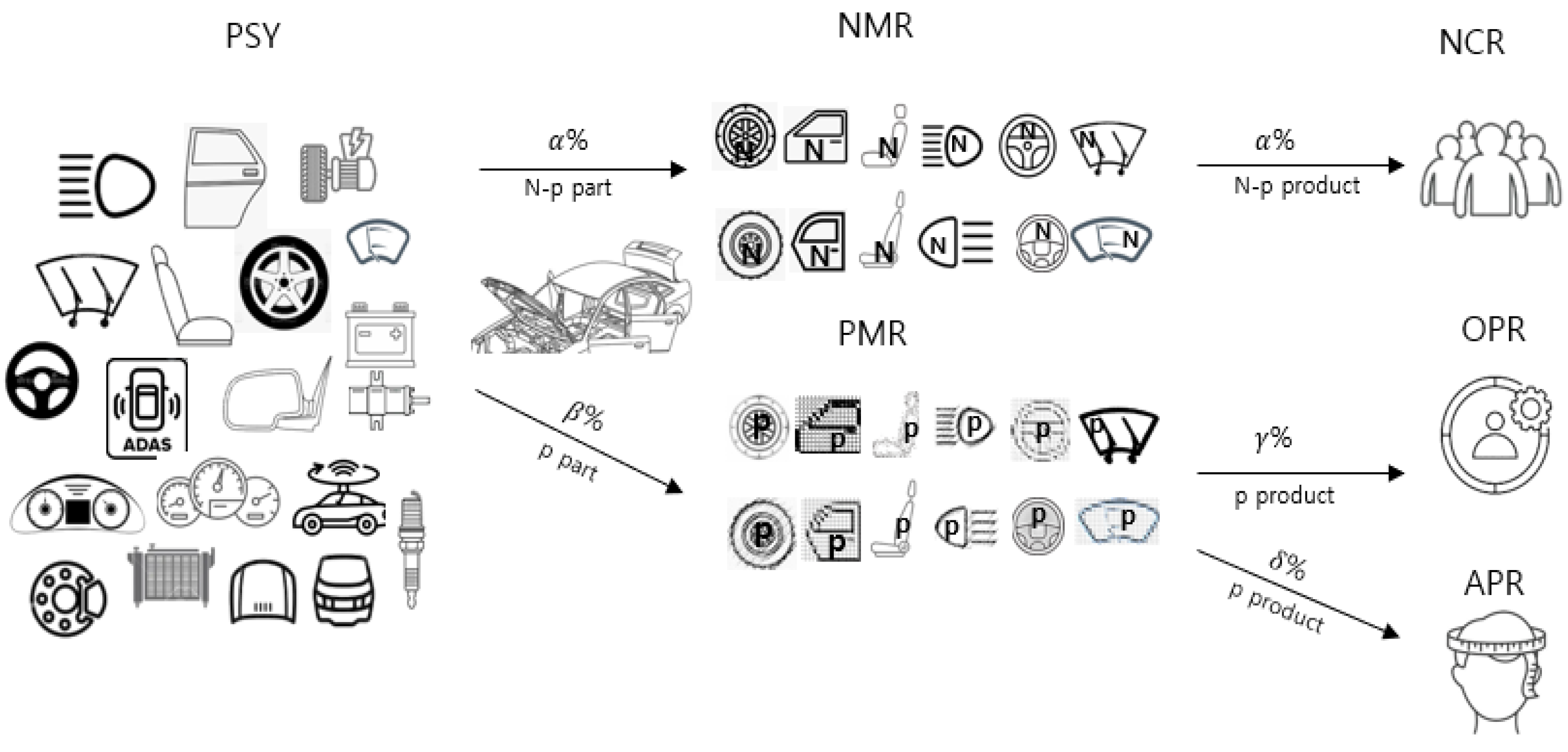
- A single product type each is produced by the NMR and PMR, respectively.
- The product is composed of different parts provided by the PSY in the previous stage.
- Non-p parts and p parts can be supplied simultaneously by the PSY.
- At least one p part is used in a product.
- The number of PSYs is fixed in advance.
- The number of NMRs and PMRs is fixed in advance.
- Only one facility is opened at each stage—PSY, NMR, and PMR.
- The operating costs of the PSY, NMR, and PMR are constant, different from each other, and known in advance.
- The unit handling costs (HCs) of each type of supplier and the manufacturer are different and known in advance.
- The unit transportation costs (TCs) of the PSY, NMR, PMR, NCR, OPR, and APR are different and known in advance.
- The number of consumers is fixed and known in advance.
- The EI for the p part is considered in the supply process, depending on the usage degree of PSY’s part.
- The EI for the p product is considered in the production process depending on the usage degree of green parts by the PMR.
- The proposed SSCN model is considered to be in a steady state.
4.1. Index Sets and Decision Variables Regarding the EI
4.1.1. Index Set for UDP and UDG of the EI
- x: index of the element probability of p parts or green p parts that can be selected by the customer in one p product.
- p: index of the maximum probability of p parts or green p parts that can be selected by the customer in one p product.
- k: index of kth variable for k.
- n: index of the sum of the number of p parts or green p parts in one p product.
- N: index of the sum of the (N-p part and p part) or (p part and green part) that can be selected by the customer in one p product.
- i: index of N-p part, , I: set of p-parts.
- i′: index of p part, , I′: set of p parts.
- j: index of N-p product, .
- j′: index of ordinary level p product, .
- k′: index of advanced level p product, .
4.1.2. Decision Variable for the UDP and UDG of the EI
- f(x): takes the value of 1 if the p part is selected and 0 otherwise.
4.2. Objective Function: Index Sets, Parameters, and Decision Variables
4.2.1. Index Set of Objective Function
- l: index of PSY, , L: set of PSYs.
- m: index of NMR, , M: set of NMRs.
- n: index of PMR, , N: set of PMRs.
- o: index of NCR, , O: set of NCRs.
- p: index of OPR, , P: set of OPRs.
- q: index of APR, , Q: set of APRs.
4.2.2. Objective Function Parameters
- : amount of N-p part i transported from PSY l.
- : amount of p part i′ transported from PSY l.
- amount of N-p product j transported from NMR m to NCR o.
- amount of ordinary p product j′ transported from PMR n to OPR p.
- amount of advanced p product k′ transported from PMR n to APR q.
- amount of N-p part i handled by PSY l.
- amount of p part i′ handled by PSY l.
- amount of N-p product j handled by NMR m for NCR o.
- amount of ordinary p product j′ handled by PMR n for OPR p.
- amount of advanced p product k′ by NMR n for APR q.
- unit TC of N-p part i from PSY l to NMR m.
- unit TC of part i′ from PSY l to PMR n.
- unit TC of N-p product j from NMR m to NCR o.
- unit TC of ordinary p product j′ from PMR n to OPR p.
- unit TC of advanced p product k′ from PMR n to APR q.
- unit HC for N-p part i at PSY l.
- unit HC for p part i′ at PSY l.
- unit HC for N-p product j at NMR m.
- unit HC for ordinary p product j′ at PMR n for OPR p.
- unit HC for advanced p product k′ at PMR n for APR q.
- FC for N-p part i at PSY l.
- FC for p product i′ at PSY l.
- FC for p product j at NMR m.
- FC for ordinary p product j′ at PMR n.
- FC for advanced p product k′ at PMR n.
- : unit CC during processing at PSY l for N-p part i.
- : unit CC during processing at PSY l for p part i′.
- : unit CC during processing at NMR m for N-p product j.
- : unit CC during processing at PMR n for ordinary p product j′.
- : unit CC during processing at PMR n for advanced p product k′.
4.2.3. Decision Variable of Objective Function
- takes a value of 1 if PSY l with N-p part i is available; 0 otherwise.
- takes a value of 1 if PSY l with p part i′ is available; 0 otherwise.
- takes a value of 1 if NMR m with N-p product j is available; 0 otherwise.
- takes a value of 1 if PMR n with ordinary p product j′ is available; 0 otherwise.
- takes a value of 1 if PMR n with advanced p product k′ is available; 0 otherwise.
5. GA-Based Approach
6. Numerical Experiments
6.1. Case Study on the UDP of the EI
6.2. Case Study of GA-Based SSCN Model Considering the ELI
- Operating system: macOS Big Sur.
- CPU: IBM-compatible PC 2.60 GHZ processor (Intel Core i7 CPU).
- RAM: 16 GB.
- Programming language: MATLAB R2021.
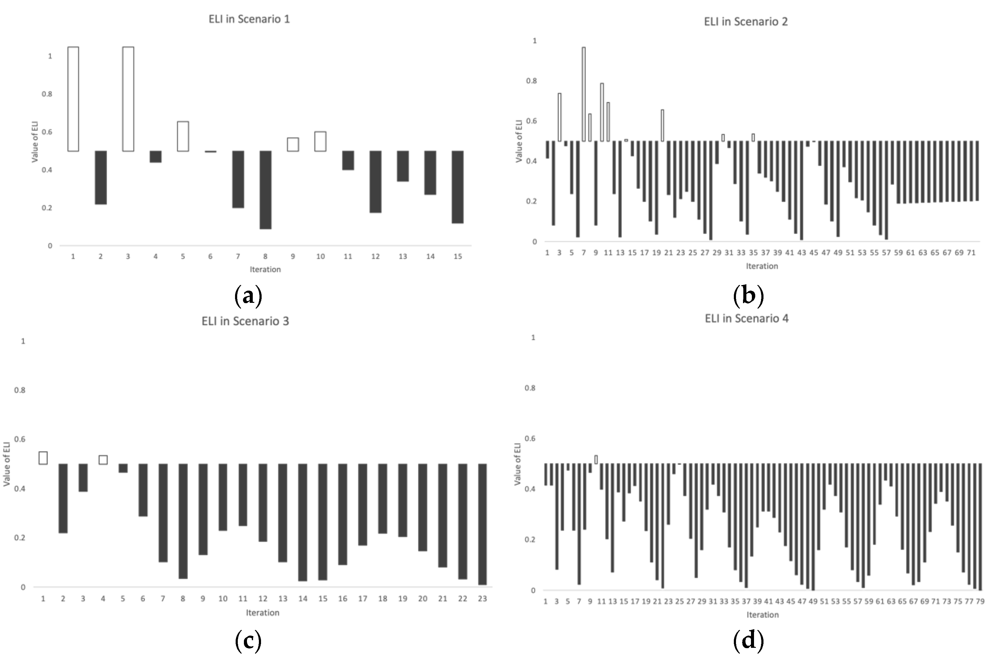
- Scenario 1. Both UDP and UDG values of less than 50%.
- Scenario 2. A value below 50% for UDP and above 50% for UDG.
- Scenario 3. A value above 50% for UDP and below 50% for UDG.
- Scenario 4. Both UDP and UDG values above 50%.
- The scientifically accurate values of the UDP and UGD can be obtained using the HD.
- Consumer preferences can be judged scientifically according to the UDP and UGD values.
- An effective evaluation system can be developed for producers to efficiently formulate production and supply chain strategies.
- Customer satisfaction can be improved by the customization of products.
- The sustainable development of enterprises can be achieved through the use of green parts.
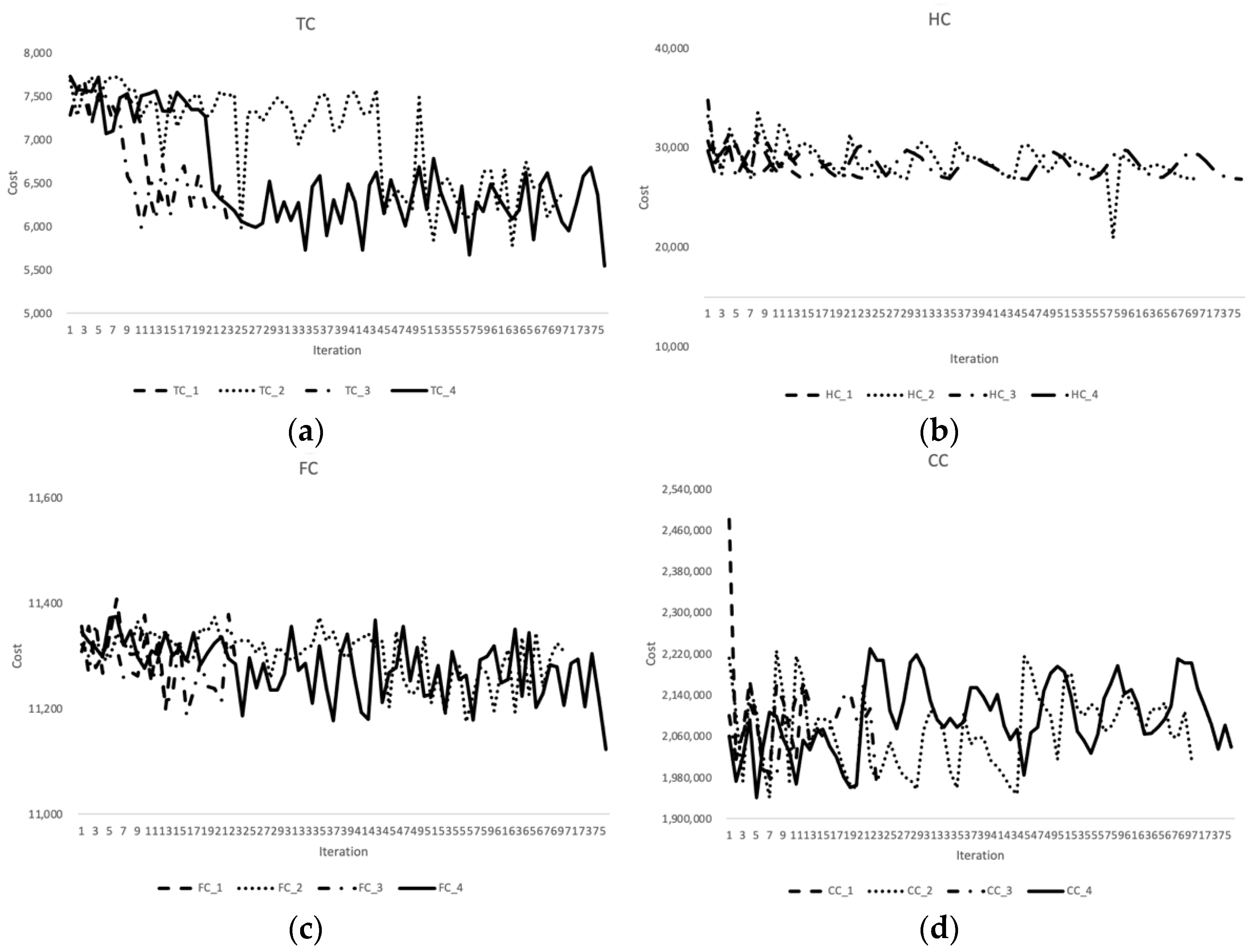
- When the ELI is determined in terms of the UDP and UDG, the corresponding TC, HC, FC, CC, and AM can be confirmed.
7. Conclusions
Author Contributions
Funding
Institutional Review Board Statement
Informed Consent Statement
Data Availability Statement
Conflicts of Interest
References
- Nurjanni, K.P.; Carvalho, M.S.; Costa, L. Green Supply Chain Design: A Mathematical Modelling Approach Based on a Multi-objective Optimization Model. Int. J. Prod. Econ. 2017, 183, 421–432. [Google Scholar] [CrossRef]
- Garetti, M.; Taisch, M. Sustainable Manufacturing: Trends and Research Challenges. Prod. Plan. Control 2012, 23, 83–104. [Google Scholar] [CrossRef]
- Machado, C.G.; Winroth, M.P.; Ribeiro da Silva, E.H.D. Sustainable Manufacturing in Industry 4.0: An Emerging Research Agenda. Int. J. Prod. Res. 2018, 58, 1462–1484. [Google Scholar] [CrossRef]
- Chen, X.; Anudari, C.; Jang, J.H. Customized Model of Cold Chain Logistics Considering Hypergeometric Distribution. J. Korean Ind. Inf. Syst. Res. 2021, 26, 37–54. [Google Scholar]
- Bandenburg, M. Low Carbon Supply Configuration for a New Product-a Goal Programming Approach. J. Prod. Res. 2015, 53, 6588–6610. [Google Scholar] [CrossRef]
- Zhao, R.; Liu, Y.; Zhang, N.; Huang, T. An Optimization Model for Green Supply Chain Management by Using a Big Data Analytic Approach. J. Clean. Prod. 2017, 142, 1085–1097. [Google Scholar] [CrossRef]
- Gerald, R.; Michael, T. Customized Supply Chain Design: Problems and alternatives for a production company in the food industry. A simulation based analysis. Int. J. Prod. Econ. 2004, 89, 217–229. [Google Scholar]
- Yao, J.M.; Gu, M.J. Optimization Analysis of Supply Chain Resource Allocation in Customized Online Shopping Service Shopping Service Mode. Math. Probl. Eng. 2015, 2015, 519125. [Google Scholar] [CrossRef]
- Liu, C.; Yao, J. Dynamic Supply Chain Integration Optimization in Service Mass Customization. Comput. Ind. Eng. 2018, 120, 42–52. [Google Scholar] [CrossRef]
- Ansari, Z.N.; Kant, R. A State-of-art Literature Review Reflecting 15 Years of Focus on Sustainable Supply Chain Management. J. Clean. Prod. 2017, 142, 2524–2543. [Google Scholar] [CrossRef]
- Hassini, E.; Surti, C.; Searcy, C. A Literature Review and A Case Study of Sustainable Supply Chain with A Focus on Metrics. Int. J. Prod. Econ. 2012, 140, 69–82. [Google Scholar] [CrossRef]
- Ahi, P.; Searcy, C. Assessing Sustainability in the Supply Chain: A Triple Bottom Line Approach. Appl. Math. Model. 2015, 39, 2882–2896. [Google Scholar] [CrossRef]
- Gao, D.; Xu, Z.; Ruan, Y.Z.; Lu, H. From a Systematic Literature Review to Integrated Definition for Sustainable Supply Chain Innovation. J. Clean. Prod. 2017, 142, 1518–1538. [Google Scholar] [CrossRef]
- Ashby, A.; Leat, M.; Smith, M.H. Making Connections: A Review of Supply Chain Management and Sustainability Literature. Supply Chain. Manag. Int. J. 2012, 17, 497–516. [Google Scholar] [CrossRef]
- Ramezankhani, M.; Torabi, S.A.; Vahidi, F. Supply Chain Performance Measurement and Evaluation: A Mixed Sustainability and Resilience Approahc. Comput. Ind. Eng. 2018, 126, 531–548. [Google Scholar] [CrossRef]
- Zhang, Q.; Shah, N.; Wassick, J.; Helling, R.; Van Egerschot, P. Sustainable Supply Chain Optimization: An Industrial Case Study. Comput. Ind. Eng. 2014, 74, 68–83. [Google Scholar] [CrossRef]
- Zhang, S.; Lee, C.K.M.; Wu, K.; Choy, K.L. Multi-objective Optimization for Sustainable Supply Chain Network Design Considering Multiple Distribution Channels. Expert Syst. Appl. 2016, 65, 87–99. [Google Scholar] [CrossRef]
- Brandenburg, M.; Govindan, K.; Sarkis, J.; Seuring, S. Quantitative Models for Sustainable Supply Chain Management: Developments and Directions. Eur. J. Oper. Res. 2014, 233, 299–312. [Google Scholar] [CrossRef]
- Ji, Y.; Li, H.H.; Zhang, H.J. Risk-Averse Two-Stage Stochastic Minimum Cost Consensus Model with Asymmetric Adjustment Cost. Group Decis. Negot. 2022, 31, 261–291. [Google Scholar] [CrossRef]
- Yun, Y.S.; Chuluunsukh, A. Green Supply Chain Network Model: Genetic Algorithm Approach. J. Korea Ind. Inf. Syst. Res. 2019, 24, 31–38. [Google Scholar]
- Vapnik, V.N. Statistical Learning Theory; Wiley: New York, NY, USA, 1998. [Google Scholar]
- Don Hush, C.S.; Clint, S. Concentration of the Hypergeometric Distribution. Stat. Probab. Lett. 2015, 75, 127–132. [Google Scholar] [CrossRef]
- Cannon, A.; Mark, E.J.; Don Hush, C.S. Machine Learning with Data Dependent Hypothesis Classes. J. Mach. Learn. Res. 2002, 2, 335–358. [Google Scholar]
- Yao, J.M.; Shi, H.Y.; Liu, C. Optimising the Configuration of Green Supply Chains under Mass Personalization. Int. J. Prod. Res. 2020, 117, 197–211. [Google Scholar]
- Mogale, D.G.; Cheikhrouhou, N.; Tiwari, M.K. Modelling of Sustainable Food Grain Supply Chain Distribution System: A bi-Objective Approach. Int. J. Prod. Res. 2020, 58, 5521–5544. [Google Scholar] [CrossRef] [Green Version]
- Kuiti, M.R.; Ghosh, D.; Gouda, S.; Swami, S.; Shankar, R. Integrated Product Design, Shelf-Space Allocation and Transportation Decision in Green Supply Chains. Int. J. Prod. Res. 2019, 57, 6181–6201. [Google Scholar] [CrossRef]
- Dolgui, A.; Ivanov, D.; Sokolov, B. Reconfigurable Supply Chain: The X-Network. Int. J. Prod. Res. 2020, 58, 4138–4163. [Google Scholar] [CrossRef]
- Hollingsworth, J.; Copeland, B.; Johnson, X.J. Are E-scooters Polluters? The Environmental Impacts of Shared Dockless Electric Scooters. Environ. Res. Lett. 2019, 14, 4–14. [Google Scholar] [CrossRef]
- Zheng, P.; Lin, Y.; Chen, C.H.; Xu, X. Smart, Connected Open Architecture Product: An IT-driven Co-creation Paradigm with Lifecycle Personalization Concerns. Int. J. Prod. Res. 2019, 57, 2571–2584. [Google Scholar] [CrossRef]
- Liu, W.; Wang, Q.; Mao, Q.; Wang, S.; Zhu, D. A Scheduling Model of Logistics Service Supply Chain Based on the Mass Customization Service and Uncertainty of FLSP’s Operation Time. Transp. Res. Part E Logist. Transp. Rev. 2015, 83, 189–215. [Google Scholar] [CrossRef]
- Tseng, M.L.; Islam, M.S.; Karia, N.; Fauzi, F.A.; Afrin, S. A Literature Review on Green Supply Chain Management: Trends and Future Challenges. Resour. Conserv. Recycl. 2019, 141, 145–162. [Google Scholar] [CrossRef]
- Qu, S.J.; Li, Y.M.; Ji, Y. The mixed integer robust maximum expert consensus models for large-scale GDM under uncertain circumstances. Appl. Soft Comput. 2021, 107, 1–13. [Google Scholar] [CrossRef]
- Krishnamoorthy, K.; Shanshan, L. Prediction Intervals for Hypergeometric Distributions. Commun. Stat. 2020, 49, 1528–1536. [Google Scholar] [CrossRef]
- Han, C.Y. The Control Method of Marine Environment Monitoring Data Quality Based on Computer. J. Coast. Res. Spec. Issue 2020, 112, 390–393. [Google Scholar] [CrossRef]
- Atan, Z.; Snyder, L.V.; Wilson, G.R. Transshipment Policies for Systems with Multiple Retailers and Two Demand Classes. OR Spectr. 2018, 40, 159–186. [Google Scholar] [CrossRef] [Green Version]
- Yan, X.; Zhao, Z.; Xiao, B. Study on Optimization of a Multi-location Inventory Model with Lateral Transshipment Considering Priority Demand. In Proceedings of the 2019 International Conference on Management Science and Industrial Engineering, New York, NY, USA, 24 May 2019; pp. 104–110. [Google Scholar]
- Van Wijk, A.; Adan, I.J.; Van Houtum, G. Optimal Lateral Transshipment Policies for Decision a Two Location Invention Problem with Multiple Demand Classes. Eur. J. Oper. Res. 2019, 272, 481–495. [Google Scholar] [CrossRef]
- Trigg, T.; Telleen, P.; Boyd, R.; Cuenot, F.; D’Ambrosio, D.; Gaghen, R.; Gagne, J.F.; Hardcastle, A.; Houssin, D.; Jones, A.R. Global EV outlook: Understanding the electric vehicle landscape to 2020. Int. Energy Agency 2013, 1, 1–40. [Google Scholar]
- Ayre, J. Electric Car Demand Growing Global Market Hits 740,000 Units. Clean Technol. 2015. Available online: http://www.bcsea.org/electric-car-demand-growing-global-market-hits-740000-units (accessed on 6 April 2020).
- Ministry of Environment. Korean Environmental Industry Statistics. Available online: http://kosis.kr/index/index.do (accessed on 6 April 2020).
- Samsun, R.; Antoni, L.; Rex, M. Report on Mobile Fuel Cell Application: Tracking Market Trends; IEA Technology Collaboration Program: Paris, France, 2020. [Google Scholar]
- Ni, H. Key Factors Influencing Electric Vehicle Sales in the United States from 2014 to 2018; Washington State University: Pullman, WA, USA, 2020. [Google Scholar]
- Zhang, X.Y.; Ming, X.G.; Liu, Z.W.; Zheng, M.K.; Qu, Y.J. A New Customization Model for Enterprise Base on Improved Framework of Customer to Business: A Case Study in Automobile Industry. Adv. Mech. Eng. 2019, 2, 1–17. [Google Scholar]
- Thomas, K. The politics of climate change in a neo-developmental state: The case of South Korea. Int. Political Sci. Rev. 2021, 42, 48–63. [Google Scholar]
- Elizabeth, A.C.; Qin, R.W.; Zlatan, H. Development of an Optimization Model to Determine Sampling Levels. Int. J. Qual. Reliab. Manag. 2016, 33, 476–487. [Google Scholar]
- Chang, Y.C.; Li, J.W.; Hsieh, S.M. Application of the Genetic Algorithm in Customization Personalized E-Course. In Proceedings of the 2010 International Conference on System Science and Engineering, Taipei, Taiwan, 1–3 July 2010; pp. 221–226. [Google Scholar]
- Jeon, N.J.; Noh, J.H.; Kim, Y.C.; Yang, W.S.; Ryu, S.C. Solvent Engineering for High-performance Inorganic-organic Hybrid Perovskite Solar Cells. Nat. Mater. 2014, 13, 897–903. [Google Scholar] [CrossRef] [PubMed]
- Gen, M.; Lin, L.; Yun, Y.S.; Inoue, H. Recent Advances in Hybrid Priority-based Genetic Algorithms for Logistics and SCM Network Design. Comput. Ind. Eng. 2018, 115, 394–412. [Google Scholar] [CrossRef]
- Chen, X. Efficient Operational Strategy of a Closed-Loop Supply Chain Network Model: Focusing on Tire Industry in Kore. Ph.D. Thesis, Chosun University, Gwangju, Korea, 2018. [Google Scholar]
- Gen, M.; Cheng, R. Genetic Algorithms and Engineering Design; John-Wiley & Sons: New York, NY, USA, 1997. [Google Scholar]
- Chakraborty, A.; Ikeda, Y. Testing “Efficient Supply Chain Propositions using Topological Characterization of the Global Supply Chain Network. PLoS ONE 2020, 15, e0239669. [Google Scholar] [CrossRef] [PubMed]
- Chuluunsukh, A.; Yun, Y.S. Supply Chain Network Design Model Considering Supplier and Route Disruptions: Hybrid Genetic Algorithm Approach. J. Korean Soc. Supply Chain Manag. 2020, 21, 37–53. [Google Scholar]


| Begin | |
| Gbt = 0 | |
| t ← 0 | //t: iteration number |
| initialize parent population GP(t) by real-number representation scheme [49]; | |
| evaluation parent population GP(t); | |
| While (not termination condition) do | |
| apply crossover operator to yield offspring population GF(t) by 2× | |
| probability crossover rate values Pcorss; | |
| apply mutation operator to yield offspring population GF(t) by 1× | |
| probability crossover rate values Pmutation; | |
| evaluation GF(t) with optimal Pcorss and Pmutation; | |
| select next GP(t) from GP(t) and GF(t) | |
| generate new GP(t) using elitist selection scheme [50]; | |
| check current best solution; | |
| t + 1 ← 0 | |
| End | |
| Output Gbt; | |
| End | |
| ELI for UDP | ELI for UDG | |||||||
|---|---|---|---|---|---|---|---|---|
| Scale | N | n | % | k | N | n | % | k |
| 1 | 10 | 5 | 0.2 | 1 | 10 | 5 | 0.4 | 2 |
| 0.4 | 2 | 0.6 | 3 | |||||
| 0.6 | 3 | 0.8 | 4 | |||||
| 2 | 20 | 10 | 0.2 | 2 | 20 | 10 | 0.4 | 4 |
| 0.4 | 4 | 0.6 | 6 | |||||
| 0.6 | 6 | 0.8 | 8 | |||||
| 3 | 30 | 15 | 0.2 | 3 | 30 | 15 | 0.4 | 6 |
| 0.4 | 6 | 0.6 | 9 | |||||
| 0.6 | 9 | 0.8 | 12 | |||||
| k | p | |||||||||||
|---|---|---|---|---|---|---|---|---|---|---|---|---|
| Scale 1 N = 10 n = 5 | 1 | 0.1 | x | 1 | ||||||||
| BUDP | 0.5 | |||||||||||
| 2 | 0.2 | x | 1 | 2 | ||||||||
| BUDP | 0.55 | 0.22 | ||||||||||
| 3 | 0.3 | x | 1 | 2 | 3 | |||||||
| BUDP | 0.416 | 0.416 | 0.083 | |||||||||
| Scale 2 N = 20 n = 10 | 2 | 0.1 | x | 1 | 2 | |||||||
| BUDP | 0.387 | 0.193 | ||||||||||
| 4 | 0.2 | x | 1 | 2 | 3 | 4 | ||||||
| BUDP | 0.268 | 0.301 | 0.201 | 0.088 | ||||||||
| 6 | 0.3 | x | 1 | 2 | 3 | 4 | 5 | 6 | ||||
| BUDP | 0.121 | 0.233 | 0.266 | 0.200 | 0.102 | 0.036 | ||||||
| Scale 3 N = 30 n = 15 | 3 | 0.1 | x | 1 | 2 | 3 | ||||||
| BUDP | 0.343 | 0.266 | 0.128 | |||||||||
| 6 | 0.2 | x | 1 | 2 | 3 | 4 | 5 | 6 | ||||
| BUDP | 0.131 | 0.230 | 0.250 | 0.187 | 0.103 | 0.025 | ||||||
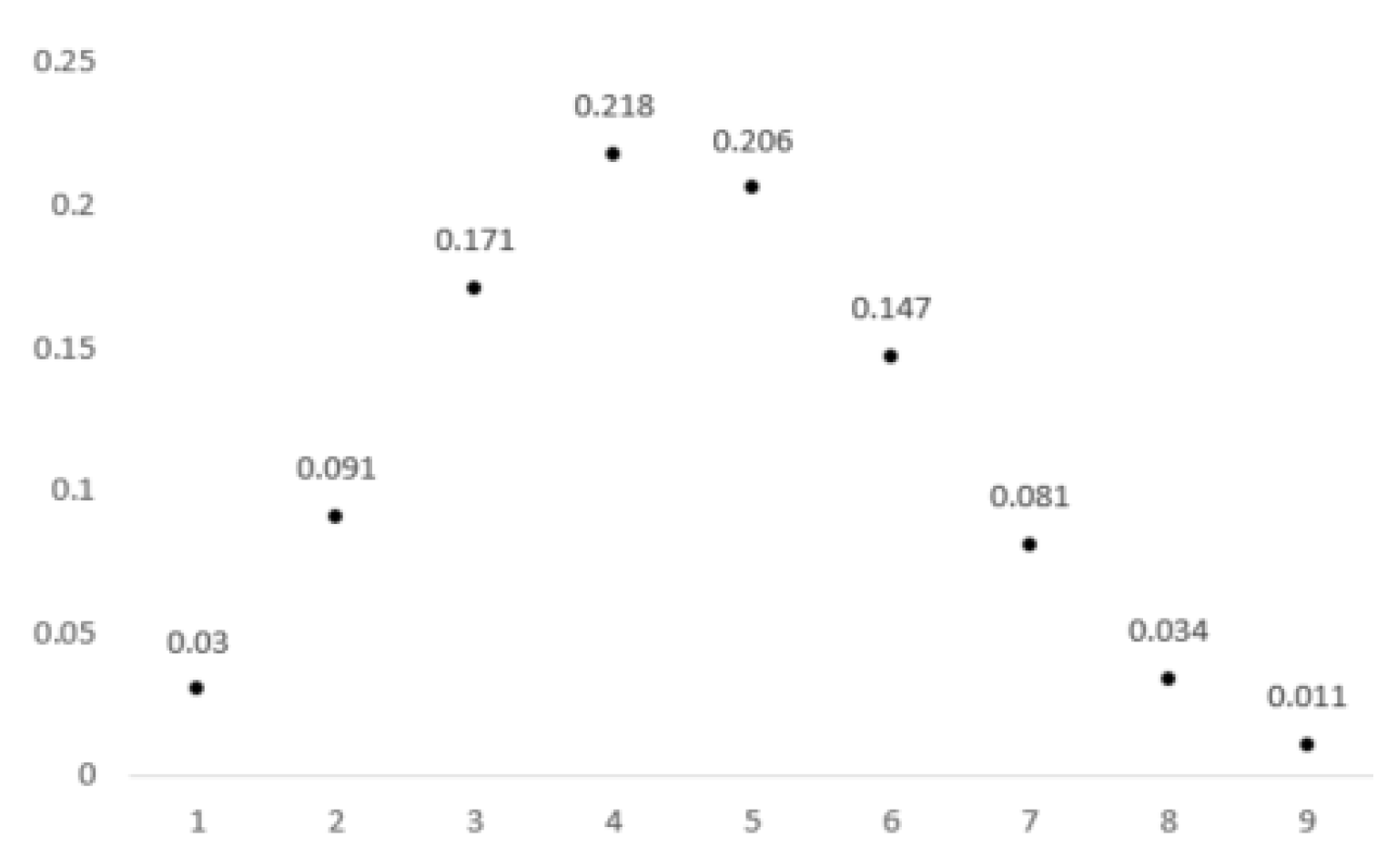
| 9 | 0.3 | x | 1 | 2 | 3 | 4 | 5 | 6 | 7 | 8 | 9 | |
| BUDP | 0.030 | 0.091 | 0.170 | 0.218 | 0.206 | 0.147 | 0.081 | 0.034 | 0.011 |
| k | p | |||||||||||
|---|---|---|---|---|---|---|---|---|---|---|---|---|
| Scale 1 N = 10 n = 5 | 2 | 0.2 | x | 1 | 2 | |||||||
| BUDG | 0.55 | 0.22 | ||||||||||
| 3 | 0.3 | x | 1 | 2 | 3 | |||||||
| BUDG | 0.416 | 0.416 | 0.083 | |||||||||
| 4 | 0.4 | x | 1 | 2 | 3 | 4 | ||||||
| BUDG | 0.238 | 0.476 | 0.238 | 0.023 | ||||||||
| Scale 2 N = 20 n = 10 | 4 | 0.2 | x | 1 | 2 | 3 | 4 | |||||
| BUDG | 0.268 | 0.301 | 0.201 | 0.088 | ||||||||
| 6 | 0.3 | x | 1 | 2 | 3 | 4 | 5 | 6 | ||||
| BUDG | 0.121 | 0.233 | 0.266 | 0.200 | 0.102 | 0.036 | ||||||
| 8 | 0.4 | x | 1 | 2 | 3 | 4 | 5 | 6 | 7 | 8 | ||
| BUDG | 0.040 | 0.120 | 0.214 | 0.250 | 0.200 | 0.111 | 0.042 | 0.010 | ||||
| Scale 3 N = 30 n = 15 | 6 | 0.2 | x | 1 | 2 | 3 | 4 | 5 | 6 | |||
| BUDG | 0.131 | 0.230 | 0.250 | 0.187 | 0.103 | 0.025 | ||||||
| 9 | 0.3 | x | 1 | 2 | 3 | 4 | 5 | 6 | 7 | 8 | 9 | |
| BUDG | 0.030 | 0.091 | 0.170 | 0.218 | 0.206 | 0.147 | 0.081 | 0.034 | 0.011 | |||
| 12 | 0.4 | x | 1 | 2 | 3 | 4 | 5 | 6 | 7 | 8 | 9 | |
| BUDG | 0.004 | 0.021 | 0.063 | 0.126 | 0.185 | 0.206 | 0.177 | 0.118 | 0.061 |
| Scale | PSY | NMR | PMR | NCR | OPR | APR |
|---|---|---|---|---|---|---|
| 1 | 3 | 5 | 5 | 1 | 3 | 3 |
| 2 | 5 | 7 | 7 | 1 | 5 | 5 |
| 3 | 10 | 14 | 14 | 1 | 10 | 10 |
| Scale | k | BUDP | X | k | BUDG | x | ||||||
|---|---|---|---|---|---|---|---|---|---|---|---|---|
| 1 | 2 | 3 | 4 | 1 | 2 | 3 | 4 | |||||
| Sacle 1 | 1 | BUDP(1) | 0.5 | 2 | BUDG(1) | 0.55 | 0.22 | |||||
| 2 | BUDP(2) | 0.55 | 0.22 | |||||||||
| Scale 2 | 2 | BUDP(3) | 0.387 | 0.193 | 4 | BUDG(2) | 0.268 | 0301 | 0.201 | 0.088 | ||
| 4 | BUDP(4) | 0.268 | 0.301 | 0.201 | 0.088 | |||||||
| Scale 3 | 3 | BUDP(5) | 0.343 | 0.266 | 0.128 | |||||||
| Scale | ELI(1) | ||||
|---|---|---|---|---|---|
| Scale 1 | BUDP(1) + BUDG(1) | 1.05(A) | 0.22(O) | ||
| BUDP(2) + BUDG(1) | 1.05(A) | 0.44(O) | |||
| Scale 2 | BUDP(3) + BUDG(2) | 0.655(A) | 0.494(O) | 0.201(O) | 0.088(O) |
| BUDP(4) + BUDG(2) | 0.569(A) | 0.602(A) | 0.402(O) | 0.176(O) | |
| Scale 3 | BUDP(5) | 0.34(O) | 0.27(O) | 0.12(O) | |
| Ordinary(O) Advanced(A) | 0 < ELI < 0.5 ELI ≥ 0.5 | ||||
| k | BUDG | x | ||||||||||||
|---|---|---|---|---|---|---|---|---|---|---|---|---|---|---|
| 1 | 2 | 3 | 4 | 5 | 6 | 7 | 8 | 9 | 10 | 11 | 12 | |||
| Sacle 1 | 3 | BUDG(1) | 0.416 | 0.416 | 0.083 | |||||||||
| 4 | BUDG(2) | 0.238 | 0.476 | 0.238 | 0.023 | |||||||||
| Scale 2 | 6 | BUDG(3) | 0.121 | 0.233 | 0.266 | 0.200 | 0.102 | 0.036 | ||||||
| 8 | BUDG(4) | 0.268 | 0.040 | 0.120 | 0.214 | 0.250 | 0.200 | 0.111 | 0.042 | 0.010 | ||||
| Scale 3 | 6 | BUDG(5) | 0.131 | 0.230 | 0.250 | 0.187 | 0.103 | 0.025 | ||||||
| 9 | BUDG(6) | 0.030 | 0.091 | 0.170 | 0.218 | 0.206 | 0.147 | 0.081 | 0.034 | 0.011 | ||||
| 12 | BUDG(7) | 0.004 | 0.021 | 0.063 | 0.126 | 0.185 | 0.206 | 0.177 | 0.118 | 0.061 | 0.024 | 0.007 | 0.001 | |
| Scale | ELI(2) | |||||||||
|---|---|---|---|---|---|---|---|---|---|---|
| Scale 1 | BUDP(1) + BUDG(1) | 0.916(A) | 0.416(O) | 0.083(A) | ||||||
| BUDP(1) + BUDG(2) | 0.738(A) | 0.476(O) | 0.238(O) | 0.023(O) | ||||||
| BUDP(2) + BUDG(1) | 0.966(A) | 0.636(A) | 0.083(O) | |||||||
| BUDP(2) + BUDG(2) | 0.788(A) | 0.693(A) | 0.238(O) | 0.023(O) | ||||||
| Scale 2 | BUDP(3) + BUDG(3) | 0.508(A) | 0.426(O) | 0.266(O) | 0.200(O) | 0.102(O) | 0.036(O) | |||
| BUDP(3) + BUDG(4) | 0.655(A) | 0.233(O) | 0.120(O) | 0.214(O) | 0.250(O) | 0.200(O) | 0.111(O) | 0.042(O) | 0.010(O) | |
| BUDP(4) + BUDG(3) | 0.389(O) | 0.534(A) | 0.467(O) | 0.288(O) | 0.102(O) | 0.036(O) | ||||
| BUDP(4) + BUDG(4) | 0.536(A) | 0.341(O) | 0.321(O) | 0.302(O) | 0.250(O) | 0.200(O) | 0.111(O) | 0.042(O) | 0.010(O) | |
| Scale 3 | BUDP(5) + BUDG(5) | 0.474(O) | 0.496(O) | 0.378(O) | 0.187(O) | 0.103(O) | 0.025(O) | |||
| BUDP(5) + BUDG(6) | 0.373(O) | 0.298(O) | 0.218(O) | 0.206(O) | 0.147(O) | 0.081(O) | 0.034(O) | 0.011(O) | ||
| BUDP(5) + BUDG(7) | 0.347(O) | 0.287(O) 0.024(O) | 0.191(O) 0.007(O) | 0.126(O) 0.001(O) | 0.185(O) | 0.206(O) | 0.177(O) | 0.118(O) | 0.061(O) | |
| Ordinary(O) Advanced(A) | 0 < ELI < 0.5 ELI ≥ 0.5 | |||||||||
| k | BUDG | x | |||||||||
|---|---|---|---|---|---|---|---|---|---|---|---|
| 1 | 2 | 3 | 4 | 5 | 6 | 7 | 8 | 9 | |||
| Scale 2 | 6 | BUDP(1) | 0.121 | 0.233 | 0.266 | 0.200 | 0.102 | 0.036 | |||
| Scale 3 | 6 | BUDP(2) | 0.131 | 0.230 | 0.250 | 0.187 | 0.103 | 0.025 | |||
| 9 | BUDP(3) | 0.030 | 0.091 | 0.170 | 0.218 | 0.206 | 0.147 | 0.081 | 0.034 | 0.011 | |
| Scale | ELI(3) | |||||||||
|---|---|---|---|---|---|---|---|---|---|---|
| Scale 1 | BUDG(1)_S1 | 0.55(A) | 0.22(O) | |||||||
| Scale 2 | BUDP(1) + BUDG(2) | 0.389(O) | 0.534(A) | 0.467(O) | 0.288(O) | 0.102(O) | 0.036(O) | |||
| Scale 3 | BUDG(2)_S1 | 0.131(O) | 0.230(O) | 0.250(O) | 0.187(O) | 0.103(O) | 0.025(O) | |||
| BUDG(3)_S1 | 0.030(O) | 0.091(O) | 0.170(O) | 0.218(O) | 0.206(O) | 0.147(O) | 0.081(O) | 0.034(O) | 0.011(O) | |
| Ordinary(O) Advanced(A) | 0 < ELI < 0.5 ELI ≥ 0.5 | |||||||||
| Scale | ELI(4) | |||||||||
|---|---|---|---|---|---|---|---|---|---|---|
| Scale 1 | BUDG(1)_S2 | 0.416(O) | 0.416(O) | 0.083(O) | ||||||
| BUDG(2)_S2 | 0.238(O) | 0.476(O) | 0.238(O) | 0.023(O) | ||||||
| Scale 2 | BUDP(1) + BUDG(3) | 0.242(O) | 0.466(O) | 0.532(A) | 0.400(O) | 0.204(O) | 0.072(O) | |||
| BUDP(1) + BUDG(4) | 0.389(O) | 0.273(O) | 0.386(O) | 0.414(O) | 0.352(O) | 0.236(O) | 0.111(O) | 0.042(O) | 0.010(O) | |
| Scale 3 | BUDP(2) + BUDG(5) | 0.262(O) | 0.460(O) | 0.500(A) | 0.374(O) | 0.206(O) | 0.050(O) | |||
| BUDP(2) + BUDG(6) | 0.161(O) | 0.321(O) | 0.420(O) | 0.374(O) | 0.309(O) | 0.172(O) | 0.081(O) | 0.034(O) | 0.011(O) | |
| BUDP(2) + BUDG(7) | 0.135(O) | 0.251(O) | 0.313(O) | 0.313(O) | 0.288(O) | 0.231(O) | 0.177(O) | 0.118(O) | 0.061(O) | |
| 0.024(O) | 0.007(O) | 0.001(O) | ||||||||
| BUDP(3) + BUDG(5) | 0.161(O) | 0.321(O) | 0.420(O) | 0.374(O) | 0.309(O) | 0.172(O) | 0.081(O) | 0.034(O) | 0.011(O) | |
| BUDP(3) + BUDG(6) | 0.060(O) | 0.182(O) | 0.340(O) | 0.436(O) | 0.412(O) | 0.294(O) | 0.162(O) | 0.068(O) | 0.022(O) | |
| BUDP(3) + BUDG(7) | 0.034(O) | 0.112(O) | 0.233(O) | 0.344(O) | 0.391(O) | 0.353(O) | 0.258(O) | 0.152(O) | 0.072(O) | |
| 0.024(O) | 0.007(O) | 0.001(O) | ||||||||
| Ordinary(O) Advanced(A) | 0 < ELI < 0.5 ELI ≥ 0.5 | |||||||||
| ELI | TC | HC | FC | CC | TTC | AM | |
|---|---|---|---|---|---|---|---|
| Scale 1 | 1.05 | 7282.5 | 34,776.2 | 11,308 | 2,481,408.4 | 2,534,775 | 6.16 |
| 0.22 | 7578 | 28,368 | 11,356 | 2,014,950 | 2,062,252 | 6.228 | |
| 0.44 | 7694 | 29,886 | 11,278 | 2,067,470 | 2,217,792 | 6.219 | |
| Scale 2 | 0.655 | 7186 | 31,370 | 11,300.3 | 2,167,935.7 | 2,217,801.9 | 6.188 |
| 0.494 | 7520 | 30,259 | 11,337.3 | 2,091,016.6 | 2,140,132.1 | 6.052 | |
| 0.201 | 7472 | 28,237 | 11,407.9 | 1,995,053 | 2,042,168.9 | 6.019 | |
| 0.088 | 7205.5 | 27,457 | 11,315.1 | 1,989,733.9 | 2,035,711.5 | 6.022 | |
| 0.569 | 7374 | 31,397 | 11,303.5 | 2,158,213.2 | 2,208,287.9 | 6.044 | |
| 0.602 | 7497.5 | 31,004 | 11,305 | 2,128,070 | 2,177,875.5 | 6.045 | |
| 0.402 | 7386 | 29,624 | 11,377.2 | 2,075,550 | 2,123,937 | 6.037 | |
| 0.176 | 7168 | 28,064 | 11,260.6 | 2,017,286.9 | 2,063,530.5 | 6.056 | |
| Scale 3 | 0.34 | 6495.5 | 29,196 | 11,334.8 | 2,167,221.4 | 2,214,247.7 | 6.18 |
| 0.27 | 6500 | 28,713 | 11,199.6 | 2,122,817.8 | 2,169,230.4 | 6.059 | |
| 0.12 | 6291 | 27,678 | 11,318.7 | 2,128,432.3 | 2,173,620 | 6.065 |
| ELI | TC | HC | FC | CC | TTC | AM | |
|---|---|---|---|---|---|---|---|
| Scale 1 | 0.916 | 7682 | 33,170 | 11,321.4 | 2,211,698 | 2,263,871 | 6.177 |
| 0.416 | 7274 | 29,720 | 11,299.6 | 2,102,618 | 2,150,911 | 6.147 | |
| 0.083 | 7566 | 27,423 | 11,325 | 1,973,439 | 2,019,753 | 6.13 | |
| 0.738 | 7718 | 31,942 | 11,312 | 2,157,764 | 2,208,736 | 6.139 | |
| 0.476 | 7438 | 30,134 | 11,295 | 2,106,658 | 2,155,525 | 6.146 | |
| 0.238 | 7694 | 28,492 | 11,342.6 | 2,006,264 | 2,053,792 | 6.129 | |
| 0.023 | 7718 | 27,009 | 11,320 | 1,941,119 | 1,987,166 | 6.122 | |
| 0.966 | 7718 | 33,515 | 11,315.2 | 2,226,848 | 2,279,396 | 6.138 | |
| 0.636 | 7578 | 31,238 | 11,365 | 2,140,998 | 2,191,179 | 6.143 | |
| 0.083 | 7578 | 27,423 | 11,332 | 1,973,439 | 2,019,772 | 6.145 | |
| 0.788 | 7262 | 32,287 | 11,347 | 2,215,334 | 2,266,230 | 6.154 | |
| 0.693 | 7438 | 31,632 | 11,334 | 2,172,409 | 2,222,813 | 6.152 | |
| 0.238 | 7426 | 28,492 | 11,347 | 2,034,544 | 2,081,809 | 6.13 | |
| 0.023 | 6783 | 30,355 | 11,322 | 2,093,528 | 2,358,026 | 6.246 | |
| Scale 2 | 0.508 | 7532 | 30,355 | 11,322 | 2,093,528 | 2,742,737 | 6.246 |
| 0.426 | 7149 | 29,789 | 11,285.4 | 2,091,205 | 2,139,428 | 6.04 | |
| 0.266 | 7353 | 28,685 | 11,298.2 | 2,044,232 | 2,091,566 | 6.046 | |
| 0.200 | 7478 | 28,230 | 11,352.5 | 1,997,659 | 2,044,725 | 6.054 | |
| 0.102 | 7520 | 27,754 | 11,346.4 | 1,965,056 | 2,011,476 | 6.072 | |
| 0.036 | 7241 | 27,098 | 11,373.2 | 1,959,419 | 2,005,041 | 6.089 | |
| 0.655 | 7341 | 31,370 | 11,328.8 | 2,159,554 | 2,209,594 | 6.022 | |
| 0.233 | 7550 | 28,458 | 11,311.6 | 2,004,749 | 2,052,109 | 6.056 | |
| 0.120 | 7508 | 27,678 | 11,326.3 | 1,972,255 | 2,018,778 | 6.09 | |
| 0.214 | 7520 | 28,327 | 11,329.5 | 2,004,965 | 2,052,141 | 6.03 | |
| 0.250 | 5984.5 | 27,023 | 11,328.5 | 2,049,684 | 2,074,039 | 6.106 | |
| 0.200 | 7319 | 28,230 | 11,305.8 | 2,008,587 | 2,055,442 | 6.539 | |
| 0.111 | 7326 | 27,616 | 11,325.7 | 1,981,923 | 2,028,191 | 6.032 | |
| 0.042 | 7211.5 | 27,140 | 11,257.8 | 1,975,258 | 2,020,867 | 6.043 | |
| 0.010 | 7356 | 26,919 | 11,316.2 | 1,956,895 | 2,002,493 | 6.054 | |
| 0.389 | 7482.5 | 29,534 | 11,305.4 | 2,070,702 | 2,119,024 | 6.055 | |
| 0.534 | 7411.5 | 30,535 | 11,291.7 | 2,110,092 | 2,159,330 | 6.078 | |
| 0.467 | 7323 | 30,072 | 11,299.9 | 2,097,812 | 2,146,507 | 6.062 | |
| 0.288 | 6949 | 28,837 | 11,313.2 | 2,065,625 | 2,110,325 | 6.044 | |
| 0.102 | 7169.5 | 27,554 | 11,320 | 1,993,336 | 2,039,379 | 6.472 | |
| 0.036 | 7241 | 27,098 | 11,373.2 | 1,959,419 | 2,005,041 | 6.089 | |
| 0.536 | 7511 | 30,548 | 11,328 | 2,102,315 | 2,151,702 | 6.078 | |
| 0.341 | 7511 | 29,203 | 11,345.4 | 2,044,057 | 2,092,116 | 6.082 | |
| 0.321 | 7100 | 29,065 | 11,306.6 | 2,059,087 | 2,106,559 | 6.085 | |
| 0.302 | 7156 | 28,934 | 11,296.4 | 2,056,132 | 2,103,519 | 6.097 | |
| 0.250 | 7496 | 28,575 | 11,328.3 | 2,013,536 | 2,060,935 | 6.475 | |
| 0.200 | 7550 | 28,230 | 11,331.6 | 2,000,204 | 2,047,316 | 6.494 | |
| 0.111 | 7302 | 27,616 | 11,342.6 | 1,981,923 | 2,028,184 | 6.48 | |
| 0.042 | 7307 | 27,140 | 11312.1 | 1960713 | 2,006,471 | 6.476 | |
| 0.010 | 7574 | 26,919 | 11,328.5 | 1,948,165 | 1,993,982 | 6.493 | |
| Scale 3 | 0.474 | 6141 | 30,121 | 11,202.6 | 2,215,254 | 2,262,388 | 6.162 |
| 0.496 | 6334 | 30,272 | 11,347.1 | 2,191,332 | 2,239,284 | 6.105 | |
| 0.387 | 6409 | 29,458 | 11,257.1 | 2,136,613 | 2,183,737 | 6.135 | |
| 0.187 | 6301 | 28,140 | 11,228 | 2,118,448 | 2,164,118 | 6.108 | |
| 0.103 | 6184 | 27,561 | 11,232.4 | 2,100,935 | 2,145,913 | 6.126 | |
| 0.025 | 7487 | 28,575 | 11,336.3 | 2,015,657 | 2,063,055 | 6.035 | |
| 0.373 | 6286 | 29,424 | 11,210.7 | 2,172,038 | 2,218,959 | 6.111 | |
| 0.298 | 5842 | 28,906 | 11,266.7 | 2,183,146 | 2,229,161 | 6.105 | |
| 0.218 | 6485 | 28,354 | 11,188.7 | 2,113,335 | 2,159,403 | 6.086 | |
| 0.206 | 6556.5 | 28,271 | 11,267.2 | 2,100,237 | 2,146,332 | 6.083 | |
| 0.147 | 6330.5 | 27,864 | 11,283.4 | 2,123,485 | 2,168,964 | 6.092 | |
| 0.081 | 6159 | 27,409 | 11,174.8 | 2,111,664 | 2,156,407 | 6.063 | |
| 0.034 | 6103 | 27,805 | 11,226.2 | 2,069,163 | 2,113,577 | 6.099 | |
| 0.011 | 6174.5 | 20,926 | 11,277.8 | 2,079,738 | 2,124,125 | 6.077 | |
| 0.347 | 6636 | 29,244 | 11,267.2 | 2,105,436 | 2,152,576 | 6.082 | |
| 0.287 | 6641 | 28,830 | 11,195.4 | 2,148,649 | 2,185,326 | 6.117 | |
| 0.191 | 6200 | 28,168 | 11,273.6 | 2,126,875 | 2,172,520 | 6.051 | |
| 0.126 | 6658 | 27,719 | 11,312.3 | 2,108,068 | 2,143,758 | 6.075 | |
| 0.185 | 5774.5 | 28,127 | 11,192.9 | 2,069,090 | 2,194,183 | 6.081 | |
| 0.206 | 6416.5 | 28,271 | 11,335 | 2,113,000 | 2,159,023 | 6.585 | |
| 0.177 | 6747 | 28,071 | 11,226.1 | 2,111,148 | 2,157,202 | 6.087 | |
| 0.118 | 6449.5 | 27,664 | 11,343.9 | 2,125,861 | 2,171,318 | 6.087 | |
| 0.061 | 6481.5 | 27,271 | 11,240.9 | 2,059,995 | 2,104,988 | 6.088 | |
| 0.024 | 6108 | 27,016 | 11,294.1 | 2,058,305 | 2,102,723 | 6.138 | |
| 0.007 | 6279 | 26,898 | 11,324.3 | 2,107,671 | 2,152,172 | 6.089 | |
| 0.001 | 6370 | 26,857 | 11,307.9 | 2,015,522 | 2,059,757 | 6.099 |
| ELI | TC | HC | FC | CC | TTC | AM | |
|---|---|---|---|---|---|---|---|
| Scale 1 | 0.55 | 7730 | 30,645 | 11,356 | 2,100,800 | 2,150,531 | 5.956 |
| 0.22 | 7561.5 | 28,368 | 11,267 | 2,017,083.1 | 2,064,279 | 6.053 | |
| Scale 2 | 0.389 | 7502 | 29,534 | 11,361.3 | 2,060,299.8 | 2,108,697 | 6.145 |
| 0.534 | 7180 | 30,535 | 11,267.5 | 2,124,232 | 2,173,213.5 | 6.055 | |
| 0.467 | 7517 | 30,072 | 11,339.9 | 2,087,771 | 2,126,699.9 | 6.078 | |
| 0.288 | 7496 | 28,837 | 11,316.6 | 2,021,414 | 2,069,063.6 | 6.051 | |
| 0.102 | 7380 | 27,554 | 11,257.4 | 1,979,196 | 2,025,386.4 | 6.082 | |
| 0.036 | 7216 | 27,098 | 11,269.8 | 1,978,879.2 | 2,024,463.1 | 6.07 | |
| Scale 3 | 0.131 | 6577 | 27,754 | 11,261.9 | 2,102,562.5 | 2,148,155.2 | 6.13 |
| 0.230 | 6432.5 | 28,437 | 11,328 | 2,088,934.3 | 2,135,131.8 | 6.073 | |
| 0.250 | 5989 | 28,575 | 11,248.6 | 2,138,069 | 2,184,081.9 | 6.086 | |
| 0.187 | 6393 | 28,140 | 11,295.8 | 2,157,244.5 | 2,203,073.4 | 6.104 | |
| 0.103 | 6083.5 | 27,561 | 11,209.4 | 2,043,197.8 | 2,088,051.7 | 6.092 | |
| 0.025 | 6712.5 | 27,023 | 11,227.4 | 2,076,519.6 | 2,121,481.5 | 6.089 | |
| 0.030 | 6125 | 27,057 | 11,334.9 | 2,059,563.5 | 2,104,080.4 | 6.069 | |
| 0.091 | 6542 | 27,478 | 11,188.3 | 2,075,187.4 | 2,120,455.7 | 6.078 | |
| 0.170 | 6700.5 | 28,023 | 11,232.4 | 2,099,058.5 | 2,205,015.4 | 6.055 | |
| 0.218 | 6210.5 | 28,354 | 11,288.3 | 2,136,517.2 | 2,182,370.1 | 6.055 | |
| 0.206 | 6591 | 28,271 | 11,242 | 2,144,433.1 | 2,190,537.5 | 6.091 | |
| 0.147 | 6228 | 27,864 | 11,238.3 | 2,093,090.4 | 2,138,420.9 | 6.119 | |
| 0.081 | 6176.5 | 27,409 | 11,214.6 | 2,089,141.4 | 2,133,941.2 | 6.103 | |
| 0.034 | 6472 | 27,085 | 11,378.4 | 2,114,194.6 | 2,159,129.5 | 6.138 | |
| 0.011 | 6104 | 26,926 | 11,290.5 | 1,959,707.4 | 2,104,027.8 | 6.131 |
| ELI | TC | HC | FC | CC | TTC | AM | |
|---|---|---|---|---|---|---|---|
| Scale 1 | 0.416 | 7730 | 29,720 | 11,345 | 2,060,198 | 2,108,993 | 6.135 |
| 0.083 | 7578 | 27,423 | 11,327.5 | 1,973,439 | 2,019,767.5 | 6.177 | |
| 0.238 | 7566 | 28,492 | 11,315 | 2,020,404 | 2,067,777 | 6.121 | |
| 0.476 | 7554 | 30,134 | 11,298 | 2,092,518 | 2,141,594 | 6.143 | |
| 0.023 | 7718 | 27,009 | 11,372.3 | 1,941,119 | 1,987,218.3 | 6.176 | |
| Scale 2 | 0.242 | 7071 | 28,520 | 11,374.7 | 2,037,212.8 | 2,084,177.6 | 6.215 |
| 0.466 | 7101 | 30,065 | 11,320.1 | 2,107,016.7 | 2,155,502.8 | 6.14 | |
| 0.532 | 7484 | 30,521 | 11,347.8 | 2,099,214.7 | 2,148,566.5 | 6.13 | |
| 0.400 | 7532 | 29,610 | 11,297.7 | 2,055,350 | 2,103,789.7 | 6.141 | |
| 0.204 | 7204 | 28,258 | 11,276.1 | 2,030,190.4 | 2,076,928.2 | 6.15 | |
| 0.072 | 7508 | 27,347 | 11,310.3 | 1,967,966 | 2,014,130.3 | 6.125 | |
| 0.389 | 7532 | 29,534 | 11,302 | 2,052,017 | 2,100,385 | 6.114 | |
| 0.273 | 7565 | 28,734 | 11,344.6 | 2,033,534 | 2,081,176.6 | 6.158 | |
| 0.386 | 7332 | 29,513 | 11,299.8 | 2,068,054.9 | 2,106,199.8 | 6.148 | |
| 0.414 | 7320 | 29,707 | 11,314.1 | 2,073,732 | 2,104,072.1 | 6.126 | |
| 0.352 | 7544 | 29,279 | 11,291.4 | 2,040,806 | 2,088,919.4 | 6.14 | |
| 0.236 | 7455.5 | 28,478 | 11,344 | 2,018,888.1 | 2,066,365.7 | 6.094 | |
| 0.111 | 7350 | 27,616 | 11,283.6 | 1,981,923 | 2,328,171.6 | 6.128 | |
| 0.042 | 7344 | 27,140 | 11,305.8 | 1,961,016 | 2,001,804.8 | 6.115 | |
| 0.010 | 7266 | 26,857 | 11,324.9 | 1,965,598.2 | 2,011,045.6 | 6.129 | |
| Scale 3 | 0.262 | 6416.5 | 28,658 | 11,335.7 | 2,134,107.8 | 2,180,517.8 | 6.151 |
| 0.460 | 6324.5 | 30,024 | 11,295.4 | 2,230,354.6 | 2,277,998.5 | 5.99 | |
| 0.500 | 6259 | 30,300 | 11,284.1 | 2,208,365 | 2,256,208.1 | 6.058 | |
| 0.374 | 6180 | 29,431 | 11,186.7 | 2,207,358.1 | 2,254,155.6 | 6.043 | |
| 0.206 | 6060 | 28,271 | 11,296.6 | 2,109,154.6 | 2,144,782.4 | 6.033 | |
| 0.050 | 6023 | 27,195 | 11,238.9 | 2,075,206.6 | 2,119,660.5 | 6.066 | |
| 0.161 | 5994 | 27,961 | 11,286 | 2,126,337.6 | 2,171,538.6 | 6.1 | |
| 0.321 | 6040 | 29,065 | 11,234.9 | 2,204,284.4 | 2,250,624.2 | 6.071 | |
| 0.420 | 6526 | 29,748 | 11,236.1 | 2,219,018.5 | 2,266,528.6 | 6.087 | |
| 0.374 | 6057.5 | 29,431 | 11,265.5 | 2,192,462 | 2,239,215 | 6.525 | |
| 0.309 | 6286 | 28,982 | 11,355.7 | 2,129,360.5 | 2,175,984.4 | 6.079 | |
| 0.172 | 6071 | 28,037 | 11,272.3 | 2,092,550.9 | 2,137,931.3 | 6.08 | |
| 0.081 | 6274.5 | 27,409 | 11,285.3 | 2,077,913.6 | 2,123,112.4 | 6.09 | |
| 0.034 | 5731 | 27,085 | 11,210.1 | 2,095,508.8 | 2,139,524.7 | 6.063 | |
| 0.011 | 6456 | 26,926 | 11,318.3 | 2,077,103.6 | 2,111,803.8 | 6.083 | |
| 0.135 | 6588.5 | 27,782 | 11,239.4 | 2,087,847.7 | 2,133,457.2 | 6.063 | |
| 0.251 | 5898.5 | 28,582 | 11,177.2 | 2,155,197.4 | 2,200,854.8 | 6.079 | |
| 0.313 | 6307 | 29,010 | 11,300.2 | 2,154,401 | 2,201,018 | 6.073 | |
| 0.288 | 6039 | 28,837 | 11,341 | 2,135,587.6 | 2,181,805.1 | 6.071 | |
| 0.231 | 6487.5 | 28,444 | 11,261.9 | 2,111,052.4 | 2,157,246 | 5.465 | |
| 0.177 | 6282.5 | 28,071 | 11,193 | 2,142,003.7 | 2,187,550.6 | 6.105 | |
| 0.118 | 5733 | 27,664 | 11,180.3 | 2,080,881.9 | 2,125,459.2 | 6.112 | |
| 0.061 | 6474 | 27,271 | 11,368.3 | 2,053,862.7 | 2,098,976.4 | 6.098 | |
| 0.024 | 6622 | 27,016 | 11,211.7 | 2,074,150.5 | 2,119,009.8 | 6.096 | |
| 0.007 | 6148 | 26,898 | 11,268 | 1,984,502.2 | 2,028,826.4 | 6.288 | |
| 0.001 | 6534.5 | 26,857 | 11,277.5 | 2,067,461.2 | 2,112,103.2 | 6.22 | |
| 0.161 | 6286 | 27,961 | 11,355.7 | 2,078,238 | 2,123,842 | 6.502 | |
| 0.321 | 6005.5 | 29,065 | 11,252.1 | 2,148,039 | 2,191,606 | 6.486 | |
| 0.420 | 6358 | 29,748 | 11,316.8 | 2,181,992 | 2,231,445 | 6.522 | |
| 0.374 | 6691.5 | 29,431 | 11,223.6 | 2,195,206 | 2,242,557 | 6.544 | |
| 0.309 | 6199.5 | 28,982 | 11,227.8 | 2,185,053 | 2,231,462 | 6.536 | |
| 0.172 | 6784.5 | 28,037 | 11,282.5 | 2,136,062 | 2,181,868 | 6.527 | |
| 0.081 | 6402 | 27,409 | 11,193.5 | 2,070,228 | 2,114,861 | 6.49 | |
| 0.034 | 6174.5 | 27,085 | 11,307.8 | 2,050,707 | 2,095,630 | 6.53 | |
| 0.011 | 5931.5 | 26,926 | 11,255.5 | 2,027,267 | 2,071,385 | 6.515 | |
| 0.060 | 6468.5 | 27,264 | 11,263.8 | 2,063,963.2 | 2,108,959 | 6.126 | |
| 0.182 | 5672.8 | 28,106 | 11,178.2 | 2,133,596.4 | 2,178,562.1 | 6.154 | |
| 0.340 | 6284.5 | 29,196 | 11,293 | 2,162,385.6 | 2,208,529.1 | 6.158 | |
| 0.436 | 6174 | 29,858 | 11,298.9 | 2,197,432.6 | 2,244,762.8 | 6.208 | |
| 0.412 | 6493 | 29,693 | 11,318.3 | 2,142,882.1 | 2,208,346 | 6.257 | |
| 0.294 | 6347.5 | 28,879 | 11,249.1 | 2,150,223.8 | 2,196,708.8 | 6.183 | |
| 0.162 | 6222.5 | 27,968 | 11,255.5 | 2,122,871.2 | 2,168,317 | 6.182 | |
| 0.068 | 6084.5 | 27,319 | 11,350.8 | 2,064,706.6 | 2,119,461.1 | 6.164 | |
| 0.022 | 6186 | 27,002 | 11,223.1 | 2,065,417.8 | 2,109,768.7 | 6.137 | |
| 0.034 | 6628 | 27,085 | 11,343.7 | 2,077,160 | 2,122,217 | 6.56 | |
| 0.112 | 5849.5 | 27,623 | 11,202.3 | 2,093,112.9 | 2,137,787.5 | 6.184 | |
| 0.233 | 6485 | 28,458 | 11,228.7 | 2,118,916.6 | 2,165,087.8 | 6.216 | |
| 0.344 | 6618.5 | 29,224 | 11,283.5 | 2,211,099.6 | 2,197,228.1 | 6.253 | |
| 0.391 | 6289 | 29,548 | 11,278.8 | 2,202,048.8 | 2,250,176.5 | 6.159 | |
| 0.353 | 6057.5 | 29,286 | 11,205.8 | 2,202,206.8 | 2,248,793.7 | 6.244 | |
| 0.258 | 5954.4 | 28,630 | 11,286.4 | 2,151,802.8 | 2,198,115.6 | 6.247 | |
| 0.152 | 6258 | 27,899 | 11,293.5 | 2,118,714.5 | 2,164,165.4 | 6.204 | |
| 0.072 | 6576.5 | 27,347 | 11,203.4 | 2,083,158.9 | 2,128,285.7 | 6.245 | |
| 0.024 | 6677.5 | 27,016 | 11,304.5 | 2,035,832 | 2,081,829 | 6.537 | |
| 0.007 | 6361 | 26,898 | 11,218.9 | 2,081,995 | 2,126,478 | 6.516 | |
| 0.001 | 5549.5 | 26,857 | 11,122.5 | 2,038,662 | 2,082,191 | 6.529 |
Publisher’s Note: MDPI stays neutral with regard to jurisdictional claims in published maps and institutional affiliations. |
© 2022 by the authors. Licensee MDPI, Basel, Switzerland. This article is an open access article distributed under the terms and conditions of the Creative Commons Attribution (CC BY) license (https://creativecommons.org/licenses/by/4.0/).
Share and Cite
Chen, X.; Jang, E. A Sustainable Supply Chain Network Model Considering Carbon Neutrality and Personalization. Sustainability 2022, 14, 4803. https://doi.org/10.3390/su14084803
Chen X, Jang E. A Sustainable Supply Chain Network Model Considering Carbon Neutrality and Personalization. Sustainability. 2022; 14(8):4803. https://doi.org/10.3390/su14084803
Chicago/Turabian StyleChen, Xing, and Eunmi Jang. 2022. "A Sustainable Supply Chain Network Model Considering Carbon Neutrality and Personalization" Sustainability 14, no. 8: 4803. https://doi.org/10.3390/su14084803
APA StyleChen, X., & Jang, E. (2022). A Sustainable Supply Chain Network Model Considering Carbon Neutrality and Personalization. Sustainability, 14(8), 4803. https://doi.org/10.3390/su14084803