
Modelling Climate Change Impacts on Tropical Dry Forest Fauna


Abstract
1. Introduction
2. Materials and Methods
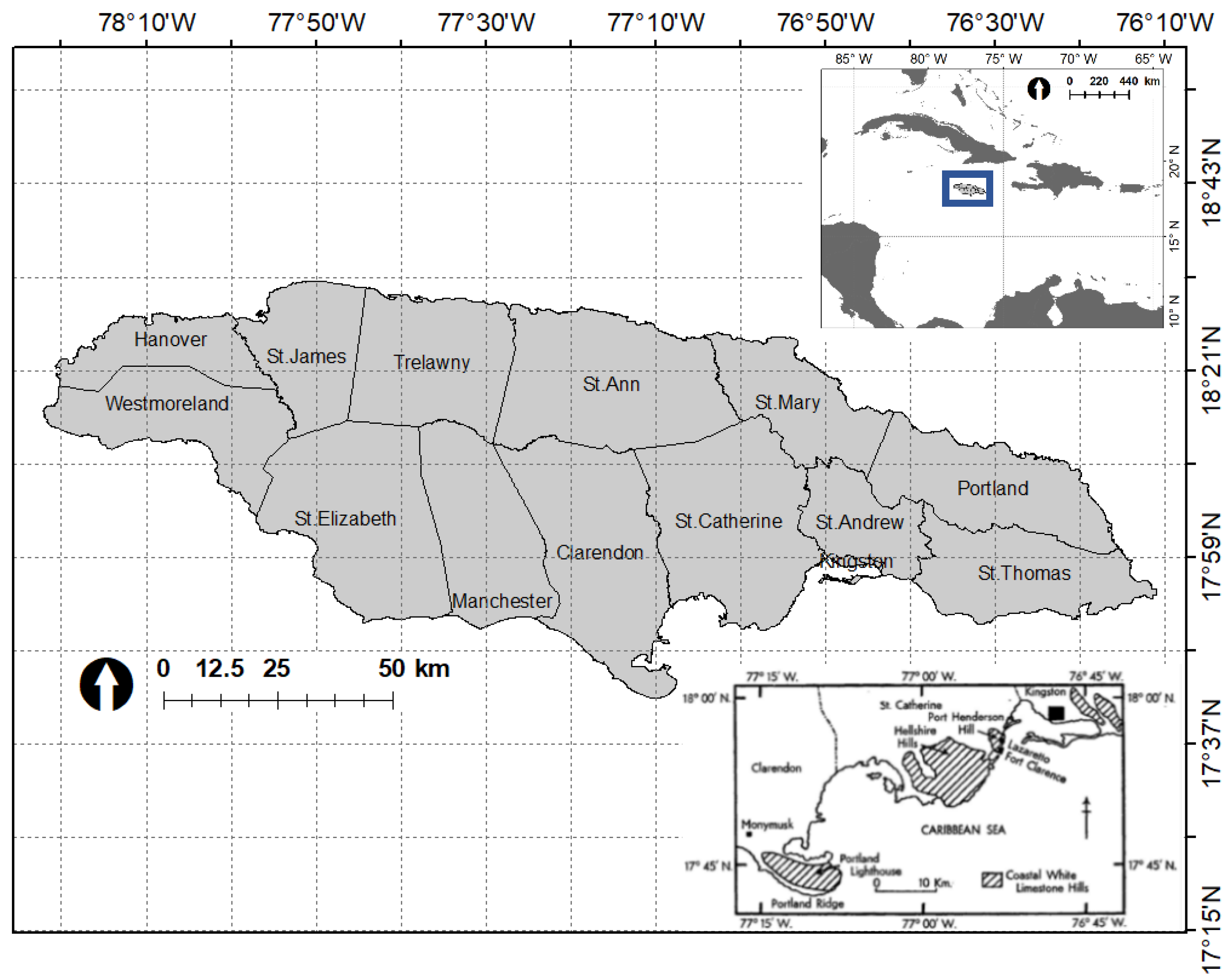
2.1. Study Site

2.2. Abundance Data
2.3. Climate Data
2.4. Model Creation
2.5. Future Projections of Abundance
3. Results
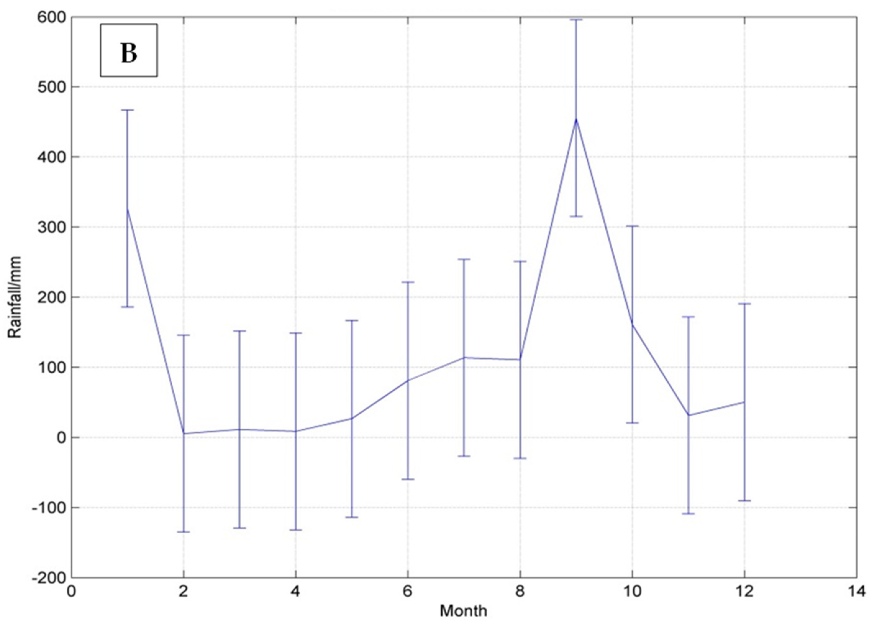
3.1. Climate of the Hellshire Hills
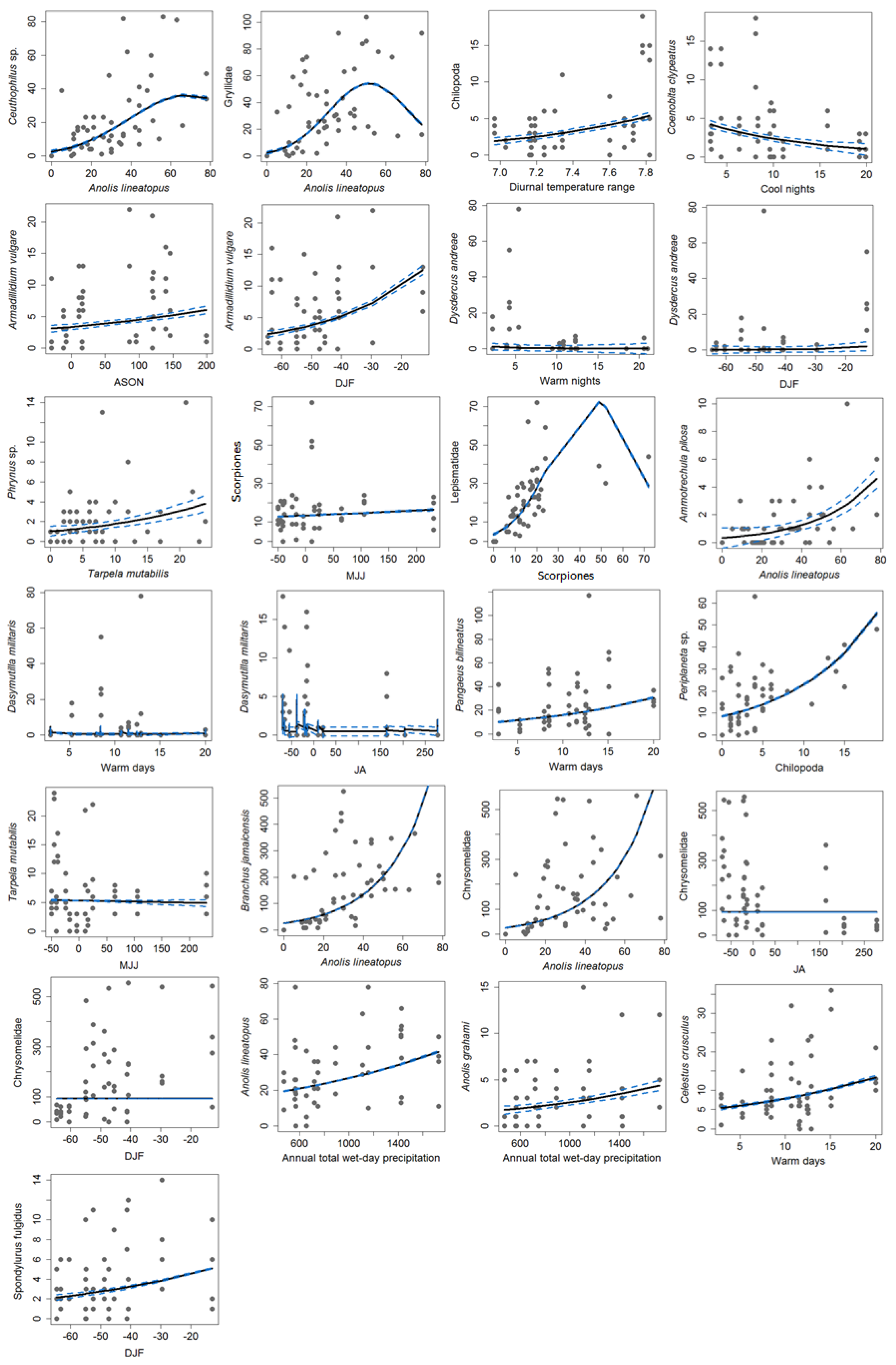
3.2. Variation in Abundance and Climate Linkages
3.3. Model Creation
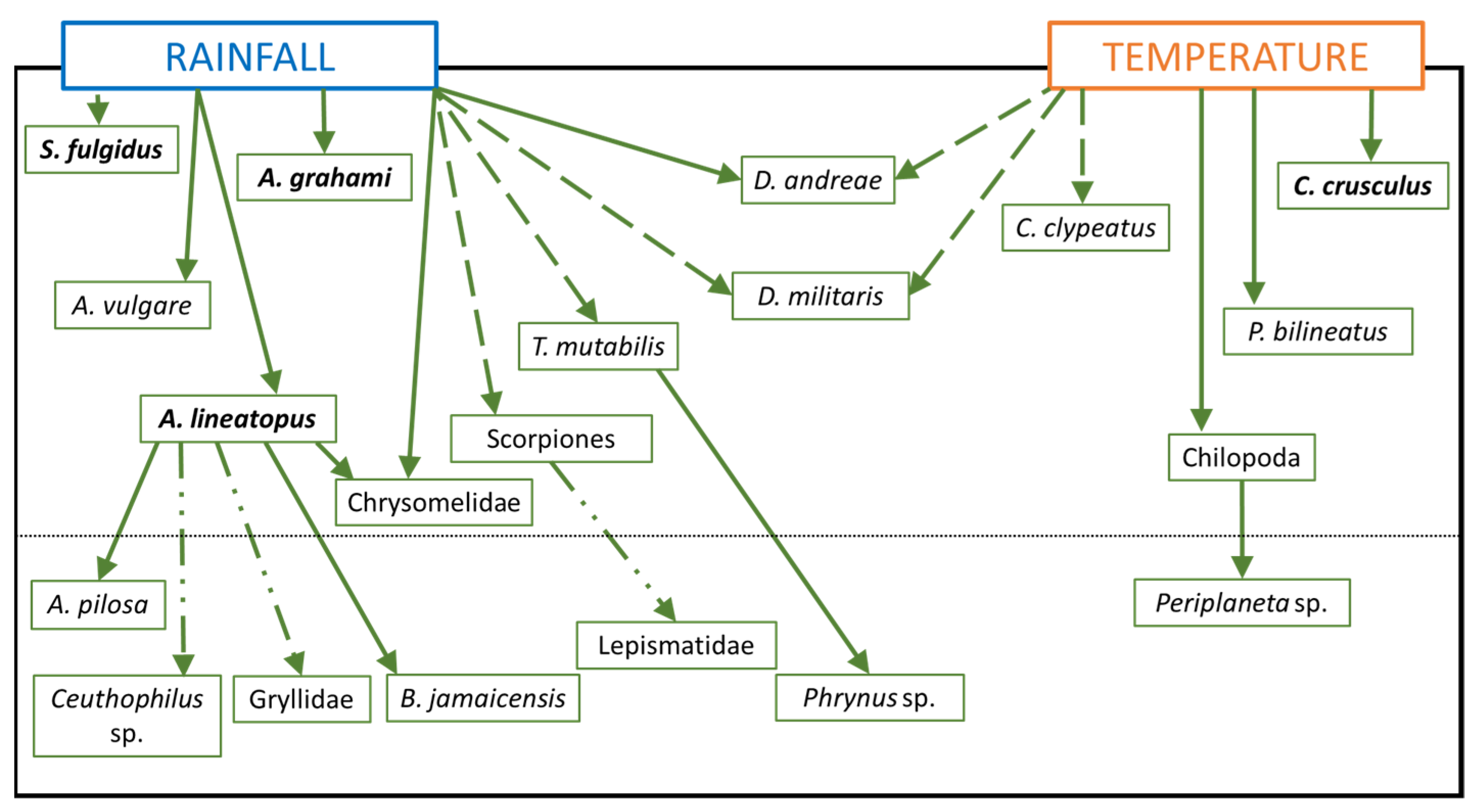
3.4. The HH Model
3.5. Model Validation
3.6. Model Projections
4. Discussion
5. Conclusions
Author Contributions
Funding
Institutional Review Board Statement
Informed Consent Statement
Data Availability Statement
Acknowledgments
Conflicts of Interest
Appendix A

| Variable | Definition | Unit | |
|---|---|---|---|
| prcptot | Annual total wet-day precipitation | Annual total PRCP in wet days (RR ≥ 1 mm) | mm |
| cdd | Consecutive dry days | Maximum number of consecutive days with RR < 1 mm | Days |
| cwd | Consecutive wet days | Maximum number of consecutive days with RR ≥ 1 mm | Days |
| R10 | Number of heavy precipitation days | Annual count of days when PRCP ≥ 10 mm | Days |
| R20 | Number of very heavy precipitation days | Annual count of days when PRCP ≥ 20 mm | Days |
| r95p | Very wet days | Annual total PRCP when RR > 95th percentile | mm |
| r99p | Extremely wet days | Annual total PRCP when RR > 99th percentile | mm |
| sdii | Simple daily intensity index | Annual total precipitation divided by the number of wet days (defined as PRCP ≥ 1.0 mm) in the year | mm/day |
| dtr | Diurnal temperature range | Monthly mean difference between TX and TN | °C |
| tmax | Maximum Tmax | Monthly maximum value of daily maximum temp | °C |
| tmin | Minimum Tmin | Monthly minimum value of daily minimum temp | °C |
| tmean | Mean Temperature | Monthly mean value of daily mean temp | °C |
| tn10p | Cool nights | Percentage of days when TN < 10th percentile | Days |
| tn90p | Warm nights | Percentage of days when TN > 90th percentile | Days |
| tx10p | Cool days | Percentage of days when TX < 10th percentile | Days |
| tx90p | Warm days | Percentage of days when TX > 90th percentile | Days |
| MJJ | Annual rainfall anomalies for the season May–June–July | mm | |
| JA | Annual rainfall anomalies for the season July–August (mid-summer drought) | mm | |
| SON | Annual rainfall anomalies for the season September–October–November | mm | |
| DJF | Annual rainfall anomalies for the season December–January–February | mm | |
References
- Pulwarty, R.S.; Nurse, L.A.; Trotz, U.O. Caribbean islands in a changing climate. Environment 2010, 52, 16–27. [Google Scholar] [CrossRef]
- Campbell, J.D.; Taylor, M.A.; Bezanilla-Morlot, A.; Stephenson, T.S.; Centella-Artola, A.; Clarke, L.A.; Stephenson, K.A. Generating Projections for the Caribbean at 1.5, 2.0, and 2.5 °C from a High-Resolution Ensemble. Atmosphere 2021, 12, 328. [Google Scholar] [CrossRef]
- Climate Studies Group Mona. The State of the Caribbean Climate; Produced for the Caribbean Development Bank; The University of the West Indies: Kingston, Jamaica, 2020. [Google Scholar]
- Stephenson, T.S.; Vincent, L.A.; Allen, T.; Van Meerbeeck, C.J.; McLean, N.; Peterson, T.C.; Taylor, M.A.; Aaron-Morrison, A.P.; Auguste, T.; Bernard, D.; et al. Changes in extreme temperature and precipitation in the Caribbean region, 1961–2010. Int. J. Climatol. 2014, 34, 2957–2971. [Google Scholar] [CrossRef]
- Torres, R.R.; Michael, N.T. Sea-level trends and interannual variability in the Caribbean Sea. J. Geophys. Res. Ocean 2013, 118, 2934–2947. [Google Scholar] [CrossRef]
- Hall, T.C.; Sealy, A.M.; Stephenson, T.S.; Kusunoki, S.; Taylor, M.A.; Chen, A.A.; Kitoh, A. Future climate of the Caribbean from a super-high-resolution atmospheric general circulation model. Theor. Appl. Climatol. 2013, 113, 271–287. [Google Scholar] [CrossRef]
- Karmalkar, A.V.; Taylor, M.A.; Campbell, J.; Stephenson, T.; New, M.; Centella, A.; Benzanilla, A.; Charlery, J. A review of observed and projected changes in climate for the islands in the Caribbean. Atmósfera 2013, 26, 283–309. [Google Scholar] [CrossRef]
- Bender, M.A.; Knutson, T.R.; Tuleya, R.E.; Sirutis, J.J.; Vecchi, G.A.; Garner, S.T.; Held, I.M. Modeled impact of anthropogenic warming on the frequency of intense Atlantic hurricanes. Science 2010, 327, 454–458. [Google Scholar] [CrossRef]
- Knutson, T.R.; McBride, J.L.; Chan, J.; Emanuel, K.; Holland, G.; Landsea, C.; Held, I.; Kossin, J.P.; Srivastava, A.K.; Sugi, M. Tropical cyclones and climate change. Nat. Geosci. 2010, 3, 157–163. [Google Scholar] [CrossRef]
- Mora, C.; Frazier, A.G.; Longman, R.J.; Dacks, R.S.; Walton, M.M.; Tong, E.J.; Sanchez, J.J.; Kaiser, L.R.; Stender, Y.O.; Anderson, J.M.; et al. The projected timing of climate departure from recent variability. Nature 2013, 502, 183–187. [Google Scholar] [CrossRef]
- Portillo-Quintero, C.A.; Sánchez-Azofeifa, G.A. Extent and conservation of tropical dry forests in the Americas. Biol. Conserv. 2010, 143, 144–155. [Google Scholar] [CrossRef]
- Nelson, H.P.; Devenish-Nelson, E.S.; Rusk, B.L.; Geary, M.; Lawrence, A.J. A call to action for climate change research on Caribbean dry forests. Reg. Environ. Change 2018, 18, 1337–1342. [Google Scholar] [CrossRef]
- Becknell, J.M.; Kucek, L.K.; Powers, J.S. Aboveground biomass in mature and secondary seasonally dry tropical forests: A literature review and global synthesis. For. Ecol. Manag. 2012, 276, 88–95. [Google Scholar] [CrossRef]
- Brandeis, T.J.; Helmer, E.H.; Marcano-Vega, H.; Lugo, A.E. Climate shapes the novel plant communities that form after deforestation in Puerto Rico and the US Virgin Islands. For. Ecol. Manag. 2009, 258, 1704–1718. [Google Scholar] [CrossRef]
- McLaren, K.P.; McDonald, M.A. The effects of moisture and shade on seed germination and seedling survival in a tropical dry forest in Jamaica. For. Ecol. Manag. 2003, 183, 61–75. [Google Scholar] [CrossRef]
- McLaren, K.P.; Lévesque, M.; Sharma, C.; Wilson, B.; McDonald, M.A. From seedlings to trees: Using ontogenetic models of growth and survivorship to assess long-term (>100 years) dynamics of a neotropical dry forest. For. Ecol. Manag. 2011, 262, 916–930. [Google Scholar] [CrossRef]
- Rojas-Sandoval, J.; Meléndez-Ackerman, E. Reproductive phenology of the Caribbean cactus Harrisia portoricensis: Rainfall and temperature associations. Botany 2011, 89, 861–871. [Google Scholar] [CrossRef]
- Jimenez-Rodríguez, D.L.; Alvarez-Añorve, M.Y.; Pineda-Cortes, M.; Flores-Puerto, J.I.; Benítez-Malvido, J.; Oyama, K.; Avila-Cabadilla, L.D. Structural and functional traits predict short term response of tropical dry forests to a high intensity hurricane. For. Ecol. Manag. 2018, 426, 101–114. [Google Scholar] [CrossRef]
- Blackie, R.; Baldauf, C.; Gautier, D.; Gumbo, D.; Kassa, H.; Parthasarathy, N.; Paumgarten, F.; Sola, P.; Pulla, S.; Waeber, P.; et al. Tropical Dry Forests: The State of Global Knowledge and Recommendations for Future Research; CIFOR: Bogor, Indonesia, 2014. [Google Scholar]
- Maharaj, S.S.; New, M. Modelling individual and collective species responses to climate change within Small Island States. Biol. Conserv. 2013, 167, 283–291. [Google Scholar] [CrossRef]
- Day, Owen, and Caribbean Natural Resources Institute. The Impacts of Climate Change on Biodiversity in Caribbean Islands: What We Know, What We Need to Know, and Building Capacity for Effective Adaptation; Caribbean Natural Resources Institute: San Juan, Trinidad and Tobago, 2009. [Google Scholar]
- Vogel, P. Seasonal hatchling recruitment and juvenile growth of the lizard Anolis lineatopus. Copeia 1984, 1984, 747–757. [Google Scholar] [CrossRef]
- Sinervo, B.; Mendez-De-La-Cruz, F.; Miles, D.B.; Heulin, B.; Bastiaans, E.; Villagrán-Santa Cruz, M.; Lara-Resendiz, R.; Martínez-Méndez, N.; Calderón-Espinosa, M.L.; Meza-Lázaro, R.N.; et al. Erosion of lizard diversity by climate change and altered thermal niches. Science 2010, 328, 894–899. [Google Scholar] [CrossRef]
- McLaren, K.; Monroe, S.; Wilson, B. The Arctic oscillation, climatic variability, and biotic factors influenced seedling dynamics in a Caribbean moist forest. Ecology 2016, 97, 2416–2435. [Google Scholar] [CrossRef]
- Cox, R.M.; Calsbeek, R. Sexually antagonistic selection, sexual dimorphism, and the resolution of intralocus sexual conflict. Am. Nat. 2009, 173, 176–187. [Google Scholar] [CrossRef]
- Gorman, G.C.; Licht, P. Seasonality in ovarian cycles among tropical Anolis lizards. Ecology 1974, 55, 360–369. [Google Scholar] [CrossRef]
- Gullan, P.J.; Cranston, P.S. The Insects: An Outline of Entomology; John Wiley & Sons: Hoboken, NJ, USA, 2014. [Google Scholar]
- Tanaka, L.K.; Tanaka, S.K. Rainfall and seasonal changes in arthropod abundance on a tropical oceanic island. Biotropica 1982, 14, 114–123. [Google Scholar] [CrossRef]
- Jackman, T.R.; Irschick, D.J.; De Queiroz, K.; Losos, J.B.; Larson, A. Molecular phylogenetic perspective on evolution of lizards of the Anolis grahami series. J. Exp. Zool. 2002, 294, 1–16. [Google Scholar] [CrossRef] [PubMed]
- Piantoni, C.; Navas, C.A.; Ibargüengoytía, N.R. Vulnerability to climate warming of four genera of New World iguanians based on their thermal ecology. Anim. Conserv. 2016, 19, 391–400. [Google Scholar] [CrossRef]
- Chown, S.L.; Gaston, K.J. Exploring links between physiology and ecology at macro-scales: The role of respiratory metabolism in insects. Biol. Rev. 1999, 74, 87–120. [Google Scholar] [CrossRef]
- Claussen, D. Studies of water loss in two species of lizards. Comp. Biochem. Physiol. 1967, 20, 115–130. [Google Scholar] [CrossRef]
- Ryan, M.J.; Latella, I.M.; Giermakowski, J.T.; Snell, H.; Poe, S.; Pangle, R.E.; Gehres, N.; Pockman, W.T.; McDowell, N.G. Too dry for lizards: Short-term rainfall influence on lizard microhabitat use in an experimental rainfall manipulation within a piñon-juniper. Funct. Ecol. 2016, 30, 964–973. [Google Scholar] [CrossRef]
- Andrew, N.R.; Hughes, L. Species diversity and structure of phytophagous beetle assemblages along a latitudinal gradient: Predicting the potential impacts of climate change. Ecol. Entomol. 2004, 29, 527–542. [Google Scholar] [CrossRef]
- Kiritani, K. Predicting impacts of global warming on population dynamics and distribution of arthropods in Japan. Popul. Ecol. 2006, 48, 5–12. [Google Scholar] [CrossRef]
- Thornthwaite, C.W. An approach toward a rational classification of climate. Geogr. Rev. 1948, 38, 55–94. [Google Scholar] [CrossRef]
- Piyaphongkul, J.; Pritchard, J.; Bale, J. Can tropical insects stand the heat? A case study with the brown planthopper Nilaparvata lugens (Stål). PLoS ONE 2012, 7, e29409. [Google Scholar] [CrossRef] [PubMed]
- Huey, R.B.; Deutsch, C.A.; Tewksbury, J.J.; Vitt, L.J.; Hertz, P.E.; Álvarez Pérez, H.J.; Garland Jr, T. Why tropical forest lizards are vulnerable to climate warming. Proc. R. Soc. B Biol. Sci. 2009, 276, 1939–1948. [Google Scholar] [CrossRef] [PubMed]
- Algar, A.C.; Mahler, D.L. Area, climate heterogeneity, and the response of climate niches to ecological opportunity in island radiations of Anolis lizards. Glob. Ecol. Biogeogr. 2016, 25, 781–791. [Google Scholar] [CrossRef]
- Kearney, M.; Shine, R.; Porter, W.P. The potential for behavioral thermoregulation to buffer “cold-blooded” animals against climate warming. Proc. Natl. Acad. Sci. USA 2009, 106, 3835–3840. [Google Scholar] [CrossRef]
- Logan, M.L.; Cox, R.M.; Calsbeek, R. Natural selection on thermal performance in a novel thermal environment. Proc. Natl. Acad. Sci. USA 2014, 111, 14165–14169. [Google Scholar] [CrossRef]
- McCluney, K.E.; Sabo, J.L. Water availability directly determines per capita consumption at two trophic levels. Ecology 2009, 90, 1463–1469. [Google Scholar] [CrossRef]
- Phillips, B.L.; Munoz, M.M.; Hatcher, A.; Macdonald, S.L.; Llewelyn, J.; Lucy, V.; Moritz, C. Heat hardening in a tropical lizard: Geographic variation explained by the predictability and variance in environmental temperatures. Funct. Ecol. 2016, 30, 1161–1168. [Google Scholar] [CrossRef]
- Wilson, B.; Grant, T.; van Veen, R.; Hudson, R.; Fleuchaus, D.; Robinson, O.; Stephenson, K. 25 Years of Conservation Effort for the Jamaican Iguana. Herpetol. Conserv. Biol. 2016, 11, 237–254. [Google Scholar]
- Wilson, B.S.; Vogel, P. A Survey of the Herpetofauna of the Hellshire Hills, Jamaica, including the Rediscovery of the Blue-tailed Galliwasp (Celestus duquesneyi Grant). Caribb. J. Sci. 2000, 36, 244–249. [Google Scholar]
- Lewis, D.S.; van Veen, R.; Wilson, B.S. Conservation implications of small Indian mongoose (Herpestes auropunctatus) predation in a hotspot within a hotspot: The Hellshire Hills, Jamaica. Biol. Invasions 2011, 13, 25–33. [Google Scholar] [CrossRef]
- Wege, D.C.; Ryan, D.; Varty, N.; Anadón-Irizarry, V.; Pérez-Leroux, A. Ecosystem Profile: The Caribbean Islands Biodiversity Hotspot; BirdLife International, Critical Ecosystem Partnership Fund: Washington, DC, USA, 2009. [Google Scholar]
- Grant, T.D. Biosphere reserve to transshipment Port: Travesty for Jamaica’s Goat Islands. IRCF Reptiles Amphib. Conserv. Nat. Hist. 2014, 21, 37–43. [Google Scholar] [CrossRef]
- Loveless, A.R.; Asprey, G.F. The Dry Evergreen Formations of Jamaica: I. The Limestone Hills of the South Coast. J. Ecol. 1957, 45, 799–822. [Google Scholar] [CrossRef]
- Wilson, B.S. Conservation of Jamaican amphibians and reptiles. In Conservation of Caribbean Island Herpetofaunas Volume 2: Regional Accounts of the West Indies; Hailey, A., Wilson, B., Horrocks, J., Eds.; Brill: Leiden, The Netherlands, 2011; Volume 2, pp. 273–310. [Google Scholar]
- R Development Core Team. R: A Language and Environment for Statistical Computing; R Foundation for Statistical Computing: Vienna, Austria, 2017. [Google Scholar]
- Simon, N.W. Core Statistics; Cambridge University Press: Cambridge, UK, 2015. [Google Scholar]
- Alexander, L.V.; Zhang, X.; Peterson, T.C.; Caesar, J.; Gleason, B.; Klein Tank, A.M.G.; Haylock, M.; Collins, D.; Trewin, B.; Rahimzadeh, F.; et al. Global observed changes in daily climate extremes of temperature and precipitation. J. Geophys. Res. Atmos. 2006, 111, D05109. [Google Scholar] [CrossRef]
- Frich, P.; Alexander, L.V.; Della-Marta, P.M.; Gleason, B.; Haylock, M.; Klein Tank, A.M.G.; Peterson, T. Observed coherent changes in Climatic Extremes During the Second Half of the Twentieth Century. Clim. Res. 2002, 19, 193–212. [Google Scholar] [CrossRef]
- Stenseth, N.C.; Ottersen, G.; Hurrell, J.W.; Mysterud, A.; Lima, M.; Chan, K.S.; Yoccoz, N.G.; Ådlandsvik, B. Studying climate effects on ecology through the use of climate indices: The North Atlantic Oscillation, El Nino Southern Oscillation and beyond. Proc. R. Soc. Lond. Ser. B Biol. Sci. 2003, 270, 2087–2096. [Google Scholar] [CrossRef]
- Calsbeek, R.; Sinervo, B. Correlational Selection on Lay Date and Life-history traits: Experimental manipulations of territory and Nest Site Quality. Evolution 2007, 61, 1071–1083. [Google Scholar] [CrossRef]
- Chen, A.A.; Taylor, M.A. Investigating the Link Between Early Season Caribbean Rainfall and the El Niño+1 Year. Int. J. Climatol. 2002, 22, 87–106. [Google Scholar] [CrossRef]
- Giannini, A.; Kushnir, Y.; Cane, M.A. Interannual variability of Caribbean rainfall, ENSO, and the Atlantic Ocean. J. Clim. 2000, 13, 297–311. [Google Scholar] [CrossRef]
- Gouirand, I.; Moron, V.; Hu, Z.Z.; Jha, B. Influence of the warm pool and cold tongue El Niños on the following Caribbean rainy season rainfall. Clim. Dyn. 2014, 42, 919–929. [Google Scholar] [CrossRef]
- Taylor, M.A.; Enfield, D.B.; Chen, A.A. Influence of the tropical Atlantic versus the tropical Pacific on Caribbean rainfall. J. Geophys. Res. Oceans 2002, 107, 10–11. [Google Scholar] [CrossRef]
- Yun, K.S.; Yeh, S.W.; Ha, K.J. Inter-El Niño variability in CMIP5 models: Model deficiencies and future changes. J. Geophys. Res. Atmos. 2016, 121, 3894–3906. [Google Scholar] [CrossRef]
- Stephenson, T.S.; Chen, A.A.; Taylor, M.A. Toward the development of prediction models for the primary Caribbean dry season. Theor. Appl. Climatol. 2008, 92, 87–101. [Google Scholar] [CrossRef]
- McLeod, A.I.; Xu, C.; Lai, Y. bestglm: Best Subset GLM and Regression Utilities, R package version 0.37.3; R Foundation for Statistical Computing: Vienna, Austria, 2020; Available online: https://CRAN.R-project.org/package=bestglm (accessed on 21 January 2022).
- McLeod, A.I.; Xu, C. bestglm: Best Subset GLM; R Package Version 0.31; R Foundation for Statistical Computing: Vienna, Austria, 2010; Available online: https://cran.r-project.org/src/contrib/Archive/bestglm/ (accessed on 21 January 2022).
- Bates, D.; Maechler, M.; Bolker, B.; Walker, S.; Christensen, R.H.B.; Singmann, H.; Dai, B.; Grothendieck, G.; Green, P.; Bolker, M.B. Package “lme4”, R package version 1.1-10; The R Project for Statistical Computin: Vienna, Austria, 2016. [Google Scholar]
- Henderson, R.W.; Powell, R. Natural History of West Indian Reptiles and Amphibians; University Press of Florida: Gainesville, FL, USA, 2009. [Google Scholar]
- Ripley, B.; Venables, B.; Bates, D.M.; Hornik, K.; Gebhardt, A.; Firth, D. Package ‘mass’. Cran R 2013, 538, 113–120. [Google Scholar]
- Barton, K. MuMIn: Multi-Model Inference, R package version 1.46.0; R Foundation for Statistical Computing: Vienna, Austria, 2022; Available online: https://CRAN.R-project.org/package=MuMIn (accessed on 21 January 2022).
- Bakar, K.S.; Sahu, S.K. spTimer: Spatio-temporal bayesian modelling using R. J. Stat. Softw. 2015, 63, 1–32. [Google Scholar] [CrossRef]
- Centella-Artola, A.; Taylor, M.A.; Bezanilla-Morlot, A.; Martinez-Castro, D.; Campbell, J.D.; Stephenson, T.S.; Vichot, A. Assessing the effect of domain size over the Caribbean region using the PRECIS regional climate model. Clim. Dyn. 2015, 44, 1901–1918. [Google Scholar] [CrossRef]
- Stephenson, K. Modelling the Impact of Climate Change on a Dry Forest Fauna. Ph.D. Thesis, The University of the West Indies, Mona Campus, Jamaica, 2017. [Google Scholar]
- Vrcibradic, D.; Rocha, C.F.D. Reproductive cycle and life-history traits of the viviparous skink Mabuya frenata in southeastern Brazil. Copeia 1998, 612–619. [Google Scholar] [CrossRef]
- Kingsbury, B.A. Thermal constraints and eurythermy in the lizard Elgaria multicarinata. Herpetologica 1994, 266–273. [Google Scholar]
- Curio, E.; Möbius, H. Versuche zum Nachweis eines Riechvermögens von Anolis l. lineatopus (Rept., Iguanidae). Z. Tierpsychol. 1978, 47, 281–292. [Google Scholar]
- Von Brockhusen-Holzer, F.; Curio, E. Ethotypic variation of prey recognition in juvenile Anolis lineatopus (Reptilia: Iguanidae). Ethology 1990, 86, 19–32. [Google Scholar] [CrossRef]
- Polis, G.A.; Myers, C.A.; Holt, R.D. The ecology and evolution of intraguild predation: Potential competitors that eat each other. Annu. Rev. Ecol. Syst. 1989, 20, 297–330. [Google Scholar] [CrossRef]
- Spiller, D.A.; Schoener, T.W. An experimental study of the effect of lizards on web-spider communities. Ecol. Monogr. 1988, 58, 57–77. [Google Scholar] [CrossRef]
- Best, T.L.; Gennaro, A.L. Feeding ecology of the lizard, Uta stansburiana, in southeastern New Mexico. J. Herpetol. 1984, 18, 291–301. [Google Scholar] [CrossRef]
- Catenazzi, A.; Brookhart, J.O.; Cushing, P.E. Natural history of coastal Peruvian solifuges with a redescription of Chinchippus peruvianus and an additional new species (Arachnida, Solifugae, Ammotrechidae). J. Arachnol. 2009, 37, 151–159. [Google Scholar] [CrossRef]
- Cloudsley-Thompson, J.L. Spiders, Scorpions, Centipedes and Mites: The Commonwealth and International Library: Biology Division; Elsevier: Amsterdam, The Netherlands, 2015. [Google Scholar]
- Chapin, K.J.; Hebets, E.A. The behavioral ecology of amblypygids. J. Arachnol. 2016, 44, 1–14. [Google Scholar] [CrossRef]
- Polis, G.A. The Biology of Scorpions; Stanford University Press: Palo Alto, CA, USA, 1990. [Google Scholar]
- Yamashita, T. Surface activity, biomass, and phenology of the striped scorpion, Centruroides vittatus (Buthidae) in Arkansas, USA. Euscorpius 2004, 17, 25–33. [Google Scholar]
- Miller, R.H.; Cameron, G.N. Effects of temperature and rainfall on populations of Armadillidium vulgare (Crustacea: Isopoda) in Texas. Am. Midl. Nat. 1987, 117, 192–198. [Google Scholar] [CrossRef]
- Warburg, M.R. Evolutionary Biology of Land Isopods; Springer Science & Business Media: Berlin/Heidelberg, Germany, 2013. [Google Scholar]
- Wolcott, G.N. The Status of Economic Entomology in Peru. Bull. Entomol. Res. 1929, 20, 225–231. [Google Scholar] [CrossRef]
- Schaefer, C.W.; Ahmad, I. Cotton stainers and their relatives (Pyrrhocoroidea: Pyrrhocoridae and Largidae). In Heteroptera of Economic Importance; CRC Press: Boca Raton, FL, USA, 2000; pp. 271–308. [Google Scholar]
- Polidori, C.; Beneitez, A.; Asís, J.D.; Tormos, J. Scramble competition by males of the velvet ant Nemka viduata (Hymenoptera: Mutillidae). Behaviour 2013, 150, 23–37. [Google Scholar]
- Vieira, C.R.; Pitts, J.; Colli, G.R. Microhabitat changes induced by edge effects impact velvet ant (Hymenoptera: Mutillidae) communities in southeastern Amazonia, Brazil. J. Insect Conserv. 2015, 19, 849–861. [Google Scholar] [CrossRef]
- Yang, S.; Liu, Z.; Xiao, Y.; Li, Y.; Rong, M.; Liang, S.; Zhang, Z.; Yu, H.; King, G.F.; Lai, R. Chemical punch packed in venoms makes centipedes excellent predators. Mol. Cell. Proteom. 2012, 11, 640–650. [Google Scholar] [CrossRef] [PubMed]
- Guizze, S.P.; Knysak, I.; Barbaro, K.C.; Karam-Gemael, M.; Chagas Jr, A. Predatory behavior of three centipede species of the order Scolopendromorpha (Arthropoda: Myriapoda: Chilopoda). Zoologia 2016, 33, e20160026. [Google Scholar] [CrossRef]
- Perez-Gelabert, D.E.; Edgecombe, G.D. Scutigeromorph centipedes (Chilopoda: Scutigeromorpha) of the Dominican Republic, Hispaniola. Novit. Caribaea 2013, 6, 36–44. [Google Scholar] [CrossRef]
- Shelley, R.M.; Sikes, D.S. Centipedes and Millipeds (Arthropoda: Diplopoda, Chilopoda) from Saba Island, Lesser Antilles, and a Consolidation of Major References on the Myriapod Fauna of “Lesser” Caribbean Islands. Insecta Mundi 2012, 742, 1–9. [Google Scholar]
- Leśniewska, M.; Jastrzębski, P.; Stańska, M.; Hajdamowicz, I. Centipede (Chilopoda) richness and diversity in the Bug River valley (Eastern Poland). ZooKeys 2015, 510, 125. [Google Scholar] [CrossRef]
- Bachvarova, D.; Doichinov, A.; Stoev, P.; Kalchev, K. Habitat preferences and effect of environmental factors on the seasonal activity of Lithobius nigripalpis L. Koch, 1867 (Chi-lopoda: Lithobiomorpha: Lithobiidae). In Proceedings of the 16th International Congress of Myriapodology, Olomouc, Czech Republic, 20–25 July 2014; p. 5. [Google Scholar]
- Cole, C.L. Stratification and survival of diapausing burrowing bugs. Southwest. Entomol. 1988, 13, 243–246. [Google Scholar]
- Riis, L.; Esbjerg, P.; Bellotti, A.C. Influence of temperature and soil moisture on some population growth parameters of Cyrtomenus bergi (Hemiptera: Cydnidae). Fla. Entomol. 2005, 88, 11–22. [Google Scholar] [CrossRef]
- Wheatly, M.G.; Burggren, W.W.; McMahon, B.R. The effects of temperature and water availability on ion and acid-base balance in hemolymph of the land hermit crab Coenobita clypeatus. Biol. Bull. 1984, 166, 427–445. [Google Scholar] [CrossRef]
- Hamasaki, K.; Kato, S.; Murakami, Y.; Dan, S.; Kitada, S. Larval growth, development and duration in terrestrial hermit crabs. Sex. Early Dev. Aquat. Org. 2015, 1, 93–107. [Google Scholar] [CrossRef]
- González, C.; Paz, A.; Ferro, C. Predicted altitudinal shifts and reduced spatial distribution of Leishmania infantum vector species under climate change scenarios in Colombia. Acta Trop. 2014, 129, 83–90. [Google Scholar] [CrossRef] [PubMed]
- Reina-Rodríguez, G.A.; Rubiano Mejía, J.E.; Castro Llanos, F.A.; Soriano, I. Orchid distribution and bioclimatic niches as a strategy to climate change in areas of tropical dry forest in Colombia. Lankesteriana 2017, 17, 17–47. [Google Scholar] [CrossRef][Green Version]
- Fain, S.J.; Quiñones, M.; Álvarez-Berríos, N.L.; Parés-Ramos, I.K.; Gould, W.A. Climate change and coffee: Assessing vulnerability by modeling future climate suitability in the Caribbean island of Puerto Rico. Clim. Change 2018, 146, 175–186. [Google Scholar] [CrossRef]


| Arthropods | |
| dbcrick | Ceuthophilus sp. |
| dhcrick | Orthoptera: Gryllidae |
| cent | Chilopoda |
| hc | Coenobita clypeatus |
| jsf | Collembola |
| pb | Armadillidium vulgare |
| rapb | Dysdercus andreae |
| bws | Phrynus sp. |
| Scorp | Scorpiones |
| sf | Lepismatidae |
| solpu | Ammotrechula pilosa |
| va | Dasymutilla militaris |
| 1bbug | Pangaeus bilineatus |
| 2bbug | Periplaneta sp. |
| 1bb | Tarpela mutabilis |
| 2bb | Branchus jamaicensis |
| sbb | Coleoptera: Chrysomelidae |
| Lizards | |
| al | Anolis lineatopus |
| ag | Anolis grahami |
| cc | Celestus crusculus |
| cd | Celestus duquesneyi |
| mm | Spondylurus fulgidus |
| Month | Rainfall | Temperature | ||
|---|---|---|---|---|
| A2 | B2 | A2 | B2 | |
| January | −39.1 | −6.6 | 3.4 | 2.3 |
| February | −18.7 | −0.8 | 4.2 | 2.5 |
| March | 16.8 | −33.8 | 4.3 | 3.6 |
| April | 10.9 | 8.7 | 3.5 | 2.8 |
| May | −52.4 | −12.4 | 4.5 | 3.0 |
| June | −65.7 | −30.0 | 5.2 | 3.1 |
| July | −57.4 | −31.0 | 5.2 | 3.1 |
| August | −51.8 | −30.7 | 4.9 | 3.0 |
| September | −61.5 | −43.3 | 5.0 | 3.1 |
| October | −67.7 | −47.3 | 4.7 | 2.8 |
| November | −43.0 | −18.5 | 3.6 | 2.4 |
| December | −53.9 | −28.7 | 3.2 | 2.4 |
| Taxa | Parameters | Estimate | SE | Z | Pr(>|z|) | mR2 | cR2 |
|---|---|---|---|---|---|---|---|
| Ceuthophilus sp. | (Intercept) | 0.903 | 0.454 | 1.988 | 0.047 | 39.4 | 51.9 |
| poly(al, degree = 2)1 | 0.078 | 0.023 | 3.485 | <0.001 | |||
| poly(al, degree = 2)2 | −0.001 | 0.000 | −2.047 | 0.041 | |||
| Gryllidae | (Intercept) | 0.816 | 0.508 | 1.605 | 0.108 | 43.0 | 47.7 |
| poly(al, degree = 2)1 | 0.124 | 0.028 | 4.457 | <0.001 | |||
| poly(al, degree = 2)2 | −0.001 | 0.000 | −3.496 | <0.001 | |||
| Chilopoda | (Intercept) | −7.913 | 3.026 | −2.615 | 0.009 | 14.9 | 17.7 |
| dtr | 1.227 | 0.407 | 3.011 | 0.003 | |||
| Coenobita clypeatus | (Intercept) | 1.718 | 0.333 | 5.154 | <0.001 | 15.0 | 15.0 |
| tn10p | −0.086 | 0.031 | −2.748 | 0.006 | |||
| Armadillidium vulgare | (Intercept) | 2.693 | 0.455 | 5.913 | <0.001 | 24.3 | 26.1 |
| ASON | 0.005 | 0.002 | 2.508 | 0.012 | |||
| DJF | 0.036 | 0.010 | 3.650 | <0.001 | |||
| Dysdercus andreae | (Intercept) | 4.272 | 1.665 | 2.566 | 0.010 | 28.2 | 28.2 |
| tn90p | −0.242 | 0.098 | −2.473 | 0.013 | |||
| DJF | 0.076 | 0.035 | 2.167 | 0.030 | |||
| Phrynus sp. | (Intercept) | 0.018 | 0.255 | 0.070 | 0.944 | 9.3 | 9.3 |
| 1bb | 0.055 | 0.024 | 2.294 | 0.022 | |||
| Scorpiones | (Intercept) | 2.650 | 0.090 | 29.451 | <0.001 | 6.4 | 6.4 |
| MJJ | −0.002 | 0.001 | −1.817 | 0.069 | |||
| Lepismatidae | (Intercept) | 1.284 | 0.257 | 4.994 | <0.001 | 58.7 | 65.5 |
| poly(scorp, degree = 2)1 | 0.130 | 0.019 | 6.891 | <0.001 | |||
| poly(scorp, degree = 2)2 | −0.001 | 0.000 | −5.270 | <0.001 | |||
| Ammotrechula pilosa | (Intercept) | −1.147 | 0.376 | −3.047 | 0.002 | 26.1 | 26.1 |
| al | 0.034 | 0.008 | 4.139 | <0.001 | |||
| Dasymutilla militaris | (Intercept) | 3.172 | 0.757 | 4.191 | <0.001 | 59.0 | 68.6 |
| tx90p | −0.286 | 0.061 | −4.681 | <0.001 | |||
| JA | −0.015 | 0.003 | −5.055 | <0.001 | |||
| Pangaeus bilineatus | (Intercept) | 2.129 | 0.362 | 5.886 | <0.001 | 8.1 | 8.1 |
| tx90p | 0.065 | 0.031 | 2.085 | 0.037 | |||
| Periplaneta sp. | (Intercept) | 2.146 | 0.167 | 12.830 | <0.001 | 21.0 | 21.0 |
| cent | 0.098 | 0.026 | 3.710 | <0.001 | |||
| Tarpela mutabilis | (Intercept) | 1.758 | 0.110 | 15.938 | <0.001 | 32.1 | 32.1 |
| MJJ | −0.007 | 0.002 | −4.044 | <0.001 | |||
| Branchus jamaicensis | (Intercept) | 3.226 | 0.303 | 10.663 | <0.001 | 34.2 | 34.2 |
| al | 0.042 | 0.008 | 5.043 | <0.001 | |||
| Chrysomelidae | (Intercept) | 4.397 | 0.633 | 6.948 | <0.001 | 48.9 | 53.4 |
| al | 0.044 | 0.008 | 5.440 | <0.001 | |||
| JA | −0.005 | 0.002 | −3.226 | 0.001 | |||
| DJF | 0.024 | 0.011 | 2.128 | 0.033 | |||
| Anolis lineatopus | (Intercept) | 2.677 | 0.283 | 9.473 | <0.001 | 11.3 | 11.3 |
| prcptot | 0.001 | 0.000 | 2.074 | 0.038 | |||
| Anolis grahami | (Intercept) | 0.175 | 0.360 | 0.486 | 0.627 | 9.1 | 9.1 |
| prcptot | 0.001 | 0.000 | 2.244 | 0.025 | |||
| Celestus crusculus | (Intercept) | 1.530 | 0.288 | 5.320 | <0.001 | 8.5 | 8.5 |
| tx90p | 0.053 | 0.024 | 2.170 | 0.030 | |||
| Spondylurus fulgidus | (Intercept) | 1.846 | 0.002 | 825.700 | <0.001 | 6.3 | 12.1 |
| DJF | 0.017 | 0.002 | 8.400 | <0.001 |
| Taxon | MSE | RMSE | MAE |
|---|---|---|---|
| Ceuthophilus sp. | 221.62 | 14.89 | 13.31 |
| Gryllidae | 341.46 | 18.48 | 15.46 |
| Chilopoda | 7.00 | 2.65 | 1.77 |
| Coenobita clypeatus | 8.62 | 2.94 | 2.00 |
| Armadillidium vulgare | 12.08 | 3.48 | 2.54 |
| Dysdercus andreae | 69.69 | 8.35 | 4.31 |
| Phrynus sp. | 3.62 | 1.90 | 1.00 |
| Scorpiones | 63.54 | 7.97 | 4.31 |
| Lepismatidae | 874.69 | 29.58 | 29.46 |
| Ammotrechula pilosa | 1.92 | 1.39 | 1.00 |
| Dasymutilla militaris | 2.77 | 1.66 | 1.23 |
| Pangaeusbilineatus | 160.54 | 12.67 | 9.62 |
| Periplaneta sp. | 76.46 | 8.74 | 7.23 |
| Tarpela mutabilis | 16.38 | 4.05 | 2.69 |
| Branchus jamaicensis | 36,259.77 | 190.42 | 119.92 |
| Chrysomelidae | 20,542.15 | 143.33 | 104.31 |
| Anolis lineatopus | 273.69 | 16.54 | 11.38 |
| Anolis grahami | 2.38 | 1.54 | 1.15 |
| Celestus crusculus | 21.62 | 4.65 | 3.46 |
| Spondylurus fulgidus | 2.69 | 1.64 | 1.31 |
| Scenario | A2 | B2 |
|---|---|---|
| Ceuthophilus sp. | 16 | <0 |
| Gryllidae | 30 | <0 |
| Chilopoda | 0 | <0 |
| Coenobita clypeatus | 0 | <0 |
| Collembola | - | - |
| Armadillidium vulgare | <0 | 10 |
| Dysdercus andreae | <0 | 129 |
| Phrynus sp. | 0 | <0 |
| Scorpiones | 1 | 6 |
| Lepismatidae | 2 | 46 |
| Ammotrechula pilosa | <0 | <0 |
| Dasymutilla militaris | 22 | <0 |
| Pangaeus bilineatus | 5 | <0 |
| Periplaneta sp. | 0 | 3 |
| Tarpela mutabilis | 1 | <0 |
| Branchus jamaicensis | <0 | 398 |
| Chrysomelidae | <0 | 2007 |
| Anolis lineatopus | <0 | 56 |
| Anolis grahami | <0 | 5 |
| Celestus crusculus | 1 | 8 |
| Celestus duquesneyi | - | - |
| Spondylurus fulgidus | <0 | 6 |
Publisher’s Note: MDPI stays neutral with regard to jurisdictional claims in published maps and institutional affiliations. |
© 2022 by the authors. Licensee MDPI, Basel, Switzerland. This article is an open access article distributed under the terms and conditions of the Creative Commons Attribution (CC BY) license (https://creativecommons.org/licenses/by/4.0/).
Share and Cite
Stephenson, K.; Wilson, B.; Taylor, M.; McLaren, K.; van Veen, R.; Kunna, J.; Campbell, J. Modelling Climate Change Impacts on Tropical Dry Forest Fauna. Sustainability 2022, 14, 4760. https://doi.org/10.3390/su14084760
Stephenson K, Wilson B, Taylor M, McLaren K, van Veen R, Kunna J, Campbell J. Modelling Climate Change Impacts on Tropical Dry Forest Fauna. Sustainability. 2022; 14(8):4760. https://doi.org/10.3390/su14084760
Chicago/Turabian StyleStephenson, Kimberly, Byron Wilson, Michael Taylor, Kurt McLaren, Rick van Veen, John Kunna, and Jayaka Campbell. 2022. "Modelling Climate Change Impacts on Tropical Dry Forest Fauna" Sustainability 14, no. 8: 4760. https://doi.org/10.3390/su14084760
APA StyleStephenson, K., Wilson, B., Taylor, M., McLaren, K., van Veen, R., Kunna, J., & Campbell, J. (2022). Modelling Climate Change Impacts on Tropical Dry Forest Fauna. Sustainability, 14(8), 4760. https://doi.org/10.3390/su14084760