1. Introduction
Even if characterized by low traffic volumes and speeds, with lower design standards than multilane roads, two-lane roads are an essential part of the road network in many countries, and are widely used for systematic and non-systematic daily travels. The roads of this type usually represent the most widespread network in a country’s transport geography. The local two-lane road network makes it possible for higher-level infrastructures (mainly roads, railways, ports, and airports) to reach the innermost areas and local markets.
This type of infrastructure has a single lane for each direction. This situation leads to a high level of interaction between vehicles traveling in the same direction, which is the scope of car-following models [
1]. The basic approach of these models considers that each driver tries to hold a desired time headway and speed behind the vehicle in front. It happens through a continuous adjustment process of braking and acceleration, influenced by driver perceptions of surroundings, perceived proximity to the desired speed, and the dynamics of the relationship with the lead vehicle [
2]. Maintaining the desired speed depends on the presence of a slower vehicle and on the possibility of overtaking maneuvers, using the opposite lane. This situation also involves a significant level of interaction between vehicles traveling in the opposite direction. Thus, the interactions between the vehicles increase with the traffic level, both in the same direction and in the opposite direction. For these reasons, the operational traffic characteristics on a two-lane road typically lead to a high level of interaction among vehicles, arising in vehicle platoons [
3]. In very general terms, the impact of platoons increases as traffic increases in both directions; the percentage of the slow vehicles increases, and then the range between the average speeds of the slow and fast vehicles widens within the traffic flow.
A deterministic threshold approach for time headways between vehicle pairs has been widely used in numerous studies, as a cut-off between free and non-free moving behavior, as summarized in recent reviews [
4,
5,
6], with values that, in most cases, are around the 3 s threshold value. This 3 s value is the headway threshold proposed by the HCM [
7] to distinguish non-follower and follower vehicles; in other words, vehicles that are free to actuate their desired speeds or not, due to slow vehicles.
It should be noted that the threshold value is assumed to be constant, even though the critical time headway that activates the vehicular interactions seems to be more appropriately a stochastic variable [
4]. Because of the traffic dynamics and vehicle interactions, time headways are crucial in road analysis for traffic quality and safety performance [
8] induced by drivers’ behaviors. Time headways have high variability within the driver population, and this variability depends on their characteristics and preferences, and the effects of the related human factors. Thus, each deterministic threshold value may appear as a simplistic and forced representation of a complex concept that needs a more accurate analysis.
Alternative and more complex methods have been introduced, based on a probabilistic identification of the status of follower vehicles, with various hypotheses regarding the probabilistic distribution of the headways [
1]. Identifying these functions and estimating their parameters, based on real-life data, do not come without difficulties in the technical applications required to analyze the functionality and performance of infrastructures [
1].
We can see without a doubt that the analysis of vehicular interactions and platoon formation on two-lane roads is a topic of ongoing interest in highway engineering. This interest responds to the need to develop significant models and indicators for performance analysis on this type of road, which is the basis for planning, upgrading, and improving transport programs to find a sustainable balance between environmental, social, and economic qualities.
Moreover, very recent works have also dealt with the topic, with particular attention paid to the presence of different vehicle categories, such as heavy-duty and commercial vehicles (HD) of different types, and connected autonomous vehicles (CAV) [
9,
10,
11].
Following this research path, in this work, we will present a model that allows us to evaluate the average percentage of vehicles which are free to travel at the desired speed and that of non-free vehicles forced to travel in platoons at lower speeds than the desired one, as a function of the traffic flow. The proposed model uses a series of statistics of the relative speed between pairs of vehicles in the traffic flow and those of their time headways. This model, the Two-Lane Roads Statistical Platooning Model, briefly TLR-SPM, allows us:
To overcome the approach that we find in a part of the technical literature, which sets a deterministic threshold for the distinction between free and non-free vehicles;
To decouple analyses from the specification of certain probabilistic distributions for the headways and the estimation of the related parameters that we can find in research works more focused on the probabilistic modelling aspects;
To have an agile but not simplistic method for evaluations in technical applications related to traffic quality assessment on two-lane roads.
The paper is organized as follows.
Section 2 frames the role of two-lane roads within the logistical infrastructure network and as part of a sustainable transport system. In
Section 3, we provide a concise literary review. In
Section 4, starting from the stochastic processes of vehicle speeds as a function of the time headway values, we specify the TRL-SPM model for estimating the leader–follower influence indices and platooning occurrence for the general case, i.e., without hypotheses on the relative distributions of probability.
Section 5 contains the description of the data processing procedure for the practical application and the explanation of the model through an example case.
Section 6 discusses the results from the perspective of the working hypotheses and of previous studies. Finally,
Section 7 contains some conclusive considerations.
2. Performance Measures and Transport Sustainability on Two-Lane Roads
There is considerable evidence that high accessibility and efficient mobility are essential for favorable social and economic development. According to a general hypothesis, as transportation is an activity derived from spatial complementarities between a supply at an origin and a demand at a destination, we can assume that economic and social activities entail transport demand [
12,
13]. This transport demand, which expresses the mobility needs of both people and goods, needs to be satisfied in the assortment of transport modes that are, from time to time, more efficient, effective, reliable, and safe. Thus, transport systems development usually occurs in parallel with social and economic growth.
Many world experiences show significant increases in traffic volumes driven by the economy’s dynamic growth, both in advanced and developing economies. The connections between the economic flows among the productive sectors, including final demand, imports, and exports, on the one hand, and the volume of passengers and goods on the different transport systems, on the other hand, are an ever-active research topic [
13]. From this point of view, a substantial coupling between economic growth and traffic growth, especially for heavy traffic (i.e., trucks and commercial vehicles), has been experienced for many years. However, recent studies have been concerned with evaluating the effects of a potential decoupling between economic growth and growth in volumes transported, linked to the efficiency of the logistics chain or the increase in value of the unit of goods transported [
12,
13].
The trend towards coupling or decoupling between the economy and volumes transported may vary, depending on the specificity of countries or regions; however, it is clear in all scenarios that the current traffic volumes are causing highly problematic congestion levels. With evidence and experience from recent years and from various parts of the world, we can say that the quality of transport infrastructure and the efficiency of logistics services impact economic and social development [
14]. Thus, the deterioration of transport systems’ performance results in significant negative repercussions on the quality of the local and global environment, human health, and individuals’ and communities’ well-being [
15].
As low-quality transportation infrastructures can highly affect environmental, social, and economic opportunities, a sustainable balance between them has become the subject of critical debate both in scientific research and in the formulation of policies and strategies, from the international to the local framework. This balance is the foundation of sustainable transport, which we can define as the provision of services and infrastructure for the mobility of people and goods in a safe, affordable, accessible, efficient, and resilient manner while minimizing emissions and environmental impacts [
16].
The road transport sector is the most common sector in which we experience recurring and nonrecurring congestion, and we can more immediately grasp its adverse effects on the environment, economy, and society. For many years, policymakers, researchers, and practitioners have implemented models for detecting, measuring, and analyzing congestion and solutions to minimize losses due to delay and costs [
17].
Thus, congestion measures and performance evaluation are the basis for upgrading and improving transport programs, considering a sustainable transport system [
17], namely: mobility, productivity, safety, reliability, and environmental impacts [
18]. According to [
18], performance measures used for traffic operations and capacity analysis on any highway facility should meet the following criteria:
Reflect road users’ perception of the quality of traffic flow;
Easy to be measured and estimated using field data;
Correlate to traffic and roadway conditions in a meaningful way;
Compatible with performance measures used on other facilities;
Able to describe both uncongested and congested conditions;
Useful in analyses concerning traffic safety, transport economics, and environmental impacts.
Two-lane roads represent a kind of interface system between the urban and interurban traffic system, making it possible for higher-level infrastructures (mainly roads, railways, ports, and airports) to reach the innermost areas and local markets, and vice versa. Thus, without a doubt, we can say that there is a need to focus on these road segments and increase their performance—reducing delays and costs—to develop effective and sustainable transport corridors.
3. Literary Review
The phenomenon of the formation of platoons makes it possible to develop significant indicators for the analysis of service performance on two-lane roads [
19].
For two-lane roads, a measure of the lost-time percentage in platoons was already introduced in the 1985 edition of the HCM [
20], as a percentage of travel time that vehicles spend in the scenario where it is impossible to overtake slower vehicles. The most up-to-date edition of the Highway Capacity Manual (HCM) [
7] proposes (especially for Class I roads, which represent the most significant extra-urban routes for traffic, and which play an important role in the local transport system and in places where the desired speeds are quite high) the use of an indicator called percent-time-spent-following (PTSF). The PTSF indicator is defined as the average percentage of the total travel time that vehicles spend in a platoon following a slower vehicle due to the inability to overtake and, in conjunction with the average travel speed (ATS), it is used to assess the level of service (LOS).
However, measuring the value of PTSF is impractical in real traffic conditions [
6] and, for this reason, HCM itself recommends the use of a surrogate measure called percent followers (PF). The PF indicator is essentially defined as the percentage of vehicles in traffic flow traveling with a follower time headway of less than or equal to 3 s.
However, some empirical studies have found that the HCM models for estimating PTSF are not aligned with the surrogate measure of PF obtained using the 3 s rule [
21,
22], and that this value usually underestimates the number of vehicles that do not enjoy the freedom of maneuvering in the traffic flow [
23]. On the other hand, research in this field is up to date, and it is always trying to test HCM methodologies with respect to actual traffic conditions and driver behavior, which may vary from country to country [
24,
25]. Washburn et al. [
6] recently defined a new methodology, based on the estimation of the free flow speed (FFS), ATS, and PF. For the PF estimate, an exponential-type function is used with slope and power coefficients obtained by applying a chain of parametric equations, depending on the length of the segment, the FFS, and the percentage of heavy vehicles moving in the opposite direction. The proposed methodology has been included in the Final Report for the NCHRP Project 17-65, with the recommendation to be included in the next edition of the HCM. Al Kaisy et al. [
18] and Washburn et al. [
6] highlight a panel of additional indicators for the assessment of vehicular interactions, based mainly on the concept underlying PTSF and PF; i.e., to estimate in some way the share of vehicles that are forced to travel in platoons due to the impossibility of overtaking using the opposite lane. As we refer to this study for specific insights, we must consider how these indicators, such as FD (follower density) and FF (follower flow), resort to the same assumption of a deterministic threshold value.
Instead of a deterministic follower time headway threshold, Al Kaisy et al. [
4] define a random variable with values within a range delimited by: a minimum, represented by the critical headway for “aggressive” vehicles that show interactions and adjust their speed in consideration of that of the previous vehicles, for low values; a maximum, represented by the critical distancing for “conservative” vehicles that manifest interactions and adjust their speed in consideration of that of the previous vehicle, for high distancing values. Al Kaisy and Durbin [
22] and Al Kaisy and Freedman [
26] offer a different estimate for the PF indicator, considering the product of the probability PP (probability of platooning), that a vehicle will be found traveling in a platoon, and the probability PI (probability of impediment), that the vehicle will be prevented from traveling at its desired speed, due to the presence of slow vehicles. In this case, PP is estimated considering the headway threshold value, while PI is estimated by measuring the average speed of slow vehicles and the probability distribution of the desired speeds for all vehicles in the flow. For the estimation of PI, the first step is to identify the leaders of the platoons by a threshold headway and to calculate their average speed. Then the second step is to estimate the distribution of the desired speeds, considering the vehicles traveling outside the platoons, because they too are identified with a threshold headway. A PI estimate is then achieved directly by intersecting the average speed of slow vehicles with the cumulative distribution of the desired speeds to find the required percentage PF = PI ∙ PP.
At the basis of this methodology, there is the need to distinguish within the platoon the vehicles that are impeded; i.e., the vehicles that are forced to maintain a speed lower than the desired one, due to the impossibility of overtaking, compared with those that are not really constrained, having their desired speed less than or equal to that of the platoon. This distinction represents one of the main weaknesses of the approach to vehicular interactions assessed using the time headway threshold value. On the one hand, any vehicle traveling with a time headway equal to or less than that threshold may be free if its desired speed is less than or equal to that of the vehicle in front of it. On the other hand, a vehicle traveling with a time headway greater than the threshold value may not be free if its desired speed is greater than that of the vehicle in front of it [
22,
26,
27].
The above problem persists even if the time headway threshold is not imposed with a priori assumptions but is obtained by estimating the probability distribution of the observed time headways in the traffic flow. Assuming that the absence of influences between following vehicles can be traced back to a Poissonian stochastic process of vehicle counts in a certain cross section of the infrastructure (i.e., with perfectly random arrivals), the reciprocal influences between vehicles are considered null if the probability density functions of the random variables that are cross-sections of the time headway process are comparable to shifted negative exponential distributions [
28]. The value of the shift interval at which this circumstance occurs can be assumed as the critical or threshold time headway. Moreover, in this case, without further information on the average relationships between the other variables of the traffic flow, we fail to consider that a group of vehicles traveling with the same time headway can generally include free and non-free behavior. In summary, the assumption of a threshold, or critical, time headway does not allow to take into full consideration the variability of the drivers’ behavior with certain vehicles, roads, and surrounding environmental conditions.
Based on these considerations, alternative methods can be introduced, based on a probabilistic identification of the status of the follower vehicle, such as the mixed-type models which propose the separation of congested situations (following, in proportion and with time headway probability distribution ) from free ones (non-following, in proportion and time headway probability distribution ) in the characterization of the overall probability distribution of the time headways .
Without prejudice to the general formulation, the separation between non-congested and congested situations that moves from
to
are the prerogative of each specific model. Among these models, we can mention Buckley’s Semi-Poisson Model [
29], Cowan’s M3 and M4 models [
30], and Branston’s Generalized Queuing Model [
31]. Chishaki and Tamura [
27] propose a method for the classification of vehicular influence situations to specify a mixed-type headway distribution model. This model [
27,
32] also allows us to analyze the influences that traffic fluctuations have on the distribution of time headways, considering a normal distribution for vehicle speeds, with variable means and variances for vehicles that travel free and not free from influences of the previous vehicle, but with constant values as the time headway varies. Catbagan and Nakamura [
23] propose a method that considers the distributions of both speeds and time headways to distinguish situations of influence/non-influence between successive vehicles. This model considers the probability that a vehicle is not free (follower) with a given speed and distance can be expressed as the product between the probability of being not free in terms of speed and being not free in terms of time headway. These two probabilities are based on suitably specified functional forms with parameters estimated by real-life data.
4. The Two-Lane Road Statistical Platooning Model
Contrary to what was mentioned above for the models by [
23,
27,
32], the approach explored in this paper does not need to hypothesize, identify, and estimate the probability laws for speeds and time headways. In fact, the in-depth analyses presented below constitute a generalization of what has already been proposed by [
27,
32], removing the assumptions of the normal distribution of the actual speeds and constancy of the means and variances of the same, relating to the values assumed by the time headways. In this way, compared to the situations discussed above, the Two-Lane Road Statistical Platooning Model (TLR-SPM) proposed here can achieve greater adaptability to experimental data, as it is not based on a priori assumptions, but on behaviors that emerge statistically from real data, and which are interpreted with a data-driven approach.
Let
A and
B be two consecutive vehicles in a single-line traffic stream, with
A (leader) preceding
B (follower). Let
and
be their velocities, and
their time headway. For each pair of vehicles
A and
B, the following three random processes with continuous amplitude and continuous parameters can be identified [
28]:
, which is the random process of the speeds implemented by the type A vehicles, with a time headway with respect to the following vehicle;
, which is the random process of the speeds implemented by the type B vehicles, with the time headway with respect to the previous vehicle;
, which is the random process of the speeds difference for the pairs of vehicles A and B, separated by the headway .
Let us consider the random variables representing, for a generic
, the cross-section of the random processes mentioned above, namely
,
, and
. For any type of random process and whatever the distributions of
,
, and
are, for the properties of the operators mean
and variance
, the following relations exist:
As varies, Equations (1) and (2) describe the mean and variance functions, respectively, of the random process of the speed difference. In general, it can be observed that if and are stationary random processes at least in a weak way, requiring only the invariance of the first two moments of the distributions of the random variables that make up the processes, is not stationary because its variance varies with a temporal trend, which depends on the covariance of the two original random processes, i.e., .
For the function
, the following limit behaviors can be identified and discussed. First, a decreasing trend is conceivable, as
increases, because, in accordance with real traffic situations, the higher the time headways, the lower the influences between the leader and the follower vehicles. The limit condition is therefore represented by:
If
A and
B travel freely at their desired speeds, as well as being null, the reciprocal influences with
, the variance of the speeds implemented by the vehicles as a function of
is constant and equal to the maximum value that the variances of the vehicle speeds of the traffic flow can assume, all other conditions being equal, i.e.,
. In other words,
is the variance of the speed distribution of vehicles when they are completely free, and therefore it can be considered:
If the vehicles are free, then, in consideration of the above, we obtain that the maximum value of the variance of the speed difference is equal to:
If, on the other hand, the vehicles do not travel at the desired speed, whether they are of type
A or
B, due to influences of various kinds, we can hypothesize the existence of a headway value
, for which the connection on average between the
and
random processes reaches its maximum. In this case, for
, the value of the covariance function
is the maximum, representing a further extreme condition in addition to Equation (3):
When the headways are similar to
, there is no longer a distinction between leading vehicles of type
A and followers of type
B. Therefore, the distributions of the relative processes of speeds
and
are also not distinguishable. Moreover, in this case, it can be assumed that for
, the variances
and
assume their minimum constant value equal to
, which is:
Then, if the vehicles are not free, for
, it can be assumed that the variance of the random process of the speed difference is minimal and is given by:
If we consider in a generic cross-section that
is the function variance
of the random process of the speed differences, its expression
as a function of
can be written as a linear combination of the variances of the relative speeds of the free vehicles
according to Equation (5) and of non-free vehicles
according to Equation (8), considering the rates
α(
τ) of the free vehicles and (1 −
α(
τ)) of the non-free vehicles:
If the function
and the values of
and
are known, with τ varying, Equation (9) can be solved with respect to
:
Let
be the random process with a discrete parameter and continuous amplitude, which associates with each traffic flow value
during a unit time interval
for all the possible determinations of the headway
between vehicles
A and
B of the same traffic flow. Moreover, let
be the probability density function of a random variable that is the generic cross-section of
. Taking a sample of
headway values obtained by observing unit flows with the same value
, group all the observed headways in classes of constant amplitude
(e.g., 1 s). If
is a generic headway value, let
be the number of headways grouped in an interval of amplitude
centered on
. When
and
are the rates of free and non-free vehicles, it results in:
which, by dividing by the sample size, becomes:
where
and
are the rates of free and non-free vehicles, respectively, traveling with the time headway
. If for constant
the number of samples
is increased indefinitely and the amplitude of the spacing interval
is decreased indefinitely, for the definition of the probability density function, it results in:
Evaluating Equation (12) for
and
, we obtain:
where
and
represent the rates of free and non-free vehicles, respectively, traveling with spacing
when the flow is
. The rates
and
for variable
are obtained by integrating
and
for values of the headway between the minimum value
compatible with the flow, and
.
If we consider the random processes of the headways concerning the free and non-free vehicles, respectively, which are
and
, the probability density functions of the generic cross-section of these random processes
and
can be obtained from the definition of the probability density function and, operating as in Equation (13), considering the ratio between the percentage of free or non-free vehicles for the headway
and flow
and the percentage of all free or non-free vehicles in the same flow
:
Thus, we have:
and therefore, by sum:
According to Equation (21), the probability density function
of the cross-section of the random process
, which associates each traffic flow value
in a unit time interval
assumed as unitary with all the possible determinations of the headway
between the vehicle types
A and
B in
, is expressed for each
as a linear combination of the probability density functions
and
, according to the rates
and
. Because
, averaging on both sides of (21) and solving with respect to
and
, we obtain:
where
,
, and
indicate the mean values for the cross-section
of the random processes
,
, and
.
6. Discussion
The results obtained for
and for the theoretical trend estimated for
with
= 5 min, which have been reported in
Figure 9, prove to be consistent with what was obtained by [
23], by applying their probabilistic model mentioned in
Section 2 to a case study in Japan.
Figure 11 shows what was obtained by [
23] for the percentage of non-free vehicles in their case study. The data set in [
23], and its empirical mean trend, overlaps the trend of
, estimated considering the Equation (33) for the case study presented by these authors.
The values obtained with Equation (33) fit very well the trend of the average values (for classes of 10 vehicles/hour) from the data from [
23] for flow rates above 300 veh/h, while they appear greater for lower flow values. In this regard, it should be noted that the minimum hourly flow rate on which Equation (33) has been estimated, in our case, is 288 veh/h, corresponding to 24 vehicles in 5 min.
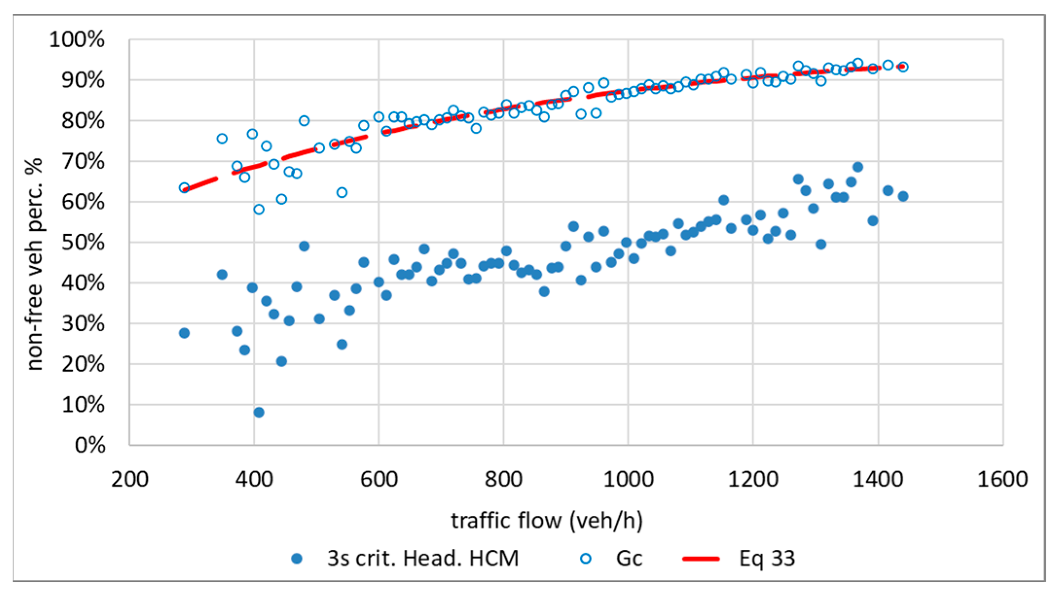
As a further comparison,
Figure 10 shows the superimposition of the results obtained for
, the trend estimated for
with Δ
t = 5, and the values of the percentage of non-free vehicles obtained by applying the 3 s headway threshold, according to the indications of the HCM for the calculation of the PF indicator.
Figure 12 shows how the percentage is largely underestimated if the 3 s critical headway is used to identify vehicles that are in non-free following situations. This circumstance is also observed by [
23]. They underline how the percentages of non-free vehicles obtained with the headway threshold seem to stabilize on percentages that are far below 100% as the traffic flow increases for values that tend to reach a maximum. This situation, which also clearly emerges in the case presented here, as shown in
Figure 12, could be related to the fact that, with an intense flow, there can be a considerable number of non-free vehicles that prefer to proceed with headways greater than 3 s, but with speeds lower than desired. It is clear that if the classification criterion is based only on the 3 s threshold, this situation of a constrained speed with a headway higher than the critical one cannot be adequately recognized and considered.
Another helpful comparison can be expressed in terms of FD [
18,
23], expressed as the product of the percentage of non-free vehicles and the estimated flow density, the latter as the ratio between hourly flow and average speed.
Figure 13 shows the FD values, as the hourly flow varies for the entire daytime period, obtained by estimating the percentage of free vehicles over 5 min intervals, alternately using Equation (33) and the 3 s threshold criterion.
In terms of the density of non-free vehicles and in an analogy to what Catbagan and Nakamura [
23] found for the Japanese case, the 3 s threshold criterion highlights the underestimated values compared to what is obtained when considering the method proposed here.
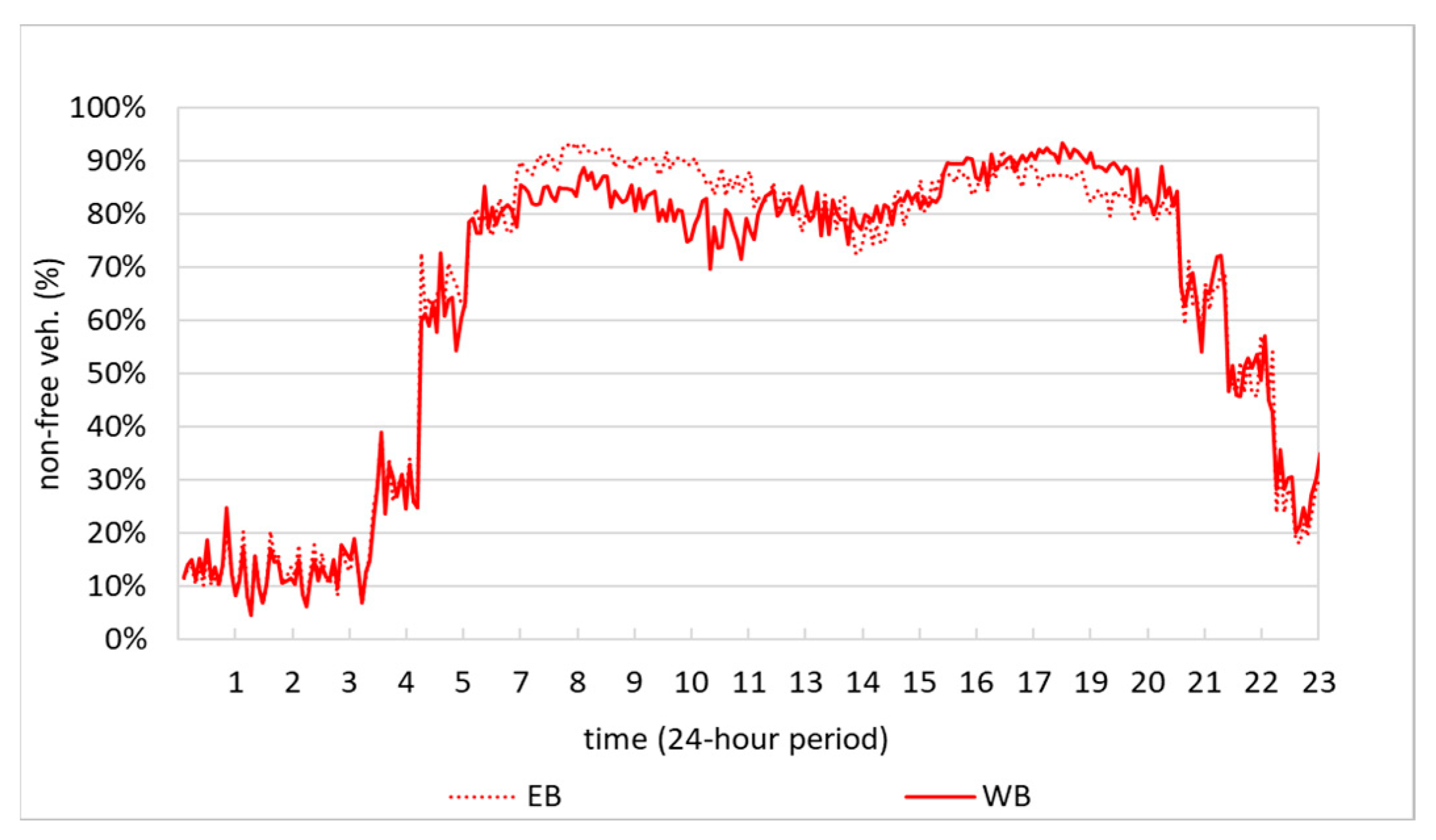
Now, if we use Equation (33) to analyze the vehicular influences starting from the whole traffic time series and aggregated with respect to a 5 min time interval, we can see an estimated percentage of non-free vehicles that remains relatively high all day long.
For the whole 24 h period, as shown in
Figure 14, the percentage of non-free vehicles is around 50%, even with hourly flows below 400 veh/h, with peaks that exceed 90% in the daytime interval. In addition to the reciprocal influences of the vehicles on the traffic flow, we can explain this evidence, considering the effects of the road geometry and the no-overtaking rule.
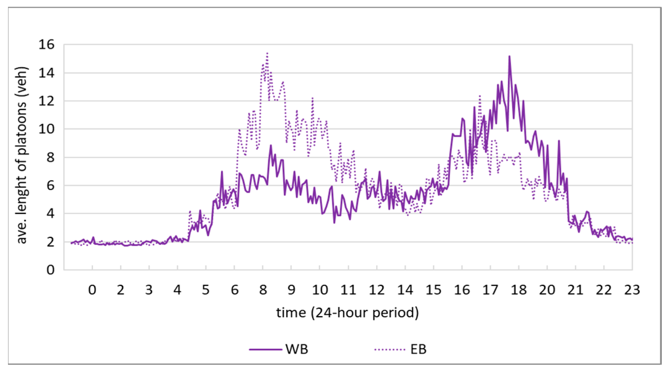
The non-free vehicle percentage estimations also allow for evaluations about the average length of the platoons. Starting from the definition by Drew [
36], we can assume that the probability that a vehicle belongs to a moving queue, or a platoon, coincides with the probability that it is not free in its behaviour. Drew’s approach [
36] to moving queues is based on a Bernoulli test, with the probability
of the presence of a queue (success) and
of the absence of a queue (failure). Assuming that the headways between the vehicles are independent, the probability
of having only one vehicle in the queue, i.e., an isolated vehicle, is equal to
, with
being the probability that the second vehicle is delayed with respect to the first by a time interval greater than the threshold (failure). Similarly, considering the third vehicle, the probability of a queue of two vehicles will be given by the combination of a success (headway less than the threshold between vehicle 2 and vehicle 1), with the probability
and a failure (headway greater than the threshold between vehicle 3 and vehicle 2) with probability
, and we will have
. We can obtain the probability of a moving tail of n vehicles from the geometric distribution
by induction.
Considering that in the case under examination,
, we will have that
The expected value of the number of vehicles in the moving queue, i.e., the average length of the platoon, as a function of the traffic flow, is therefore given by
.
Figure 15 shows the trend of the average length of the platoon for the entire day in both directions for 5 min intervals. In this case, we can see that the no-overtaking rule determines that there are two vehicle platoons, even with meager traffic.
The Effects of the Elimination of the No-Overtaking Rule in a Downstream Section
Interesting elements for the discussion can appear by simulating the effect of eliminating the no-overtaking rule in a downstream cross-section of the road in both travel directions. Thus, we can calculate the probability
that a vehicle can overtake another in front of it as a function of the flow
on the opposite lane and
on the same lane. The percentage of non-free vehicles in a downstream section where overtaking is allowed can be obtained as the product of the non-free vehicle percentage
upstream and the percentage
of vehicles that cannot overtake downstream. The probability
can be estimated by considering the product between the probability
of having a gap greater than a minimum value needed for the overtaking maneuver in oncoming traffic, and the probability
of having a gap greater than a minimum safety value for merging the right lane. The minimum time gap
for passing may be considered equal to twice the average duration of an overtaking maneuver [
37]. Considering for the latter a value equal to 6 s, as in Vlahogianni’s studies for this type of road [
38], we can assume
= 12 s, which corresponds to the total time of the overtaking maneuver phases according to the Italian model [
19], which is equal to 10 s [
39,
40] and which is increased by 20%. The minimum time gap
for merging the right lane can be assumed to be equal to 8 s, in such a way as to ensure an adequate headway of approximately 4 s with respect to the previous and following vehicle when merging into the right lane. Considering a headway distribution in the two traffic streams according to [
28] as:
- 8.
A negative exponential distribution for flows up to 300 veh/h;
- 9.
An Erlang distribution for flows greater than 300 veh/h;
the probability of having a gap
greater than or equal to
= 12 s for the overcoming and
= 8 s for the merging traffic flow can be calculated with the expressions:
The values of hourly traffic, the parameter k, and the probability of overtaking and merging the lane are shown in
Table 1, using the relationship
as was indicated by [
28]. The probability values in
Table 1 show the evident reduction of the percentage of overtaking
and merging in the lane
as the traffic flow
increases, due to the reduction of acceptable headways in consideration of the safety thresholds that we have assumed (
= 12 s and
= 12 s).
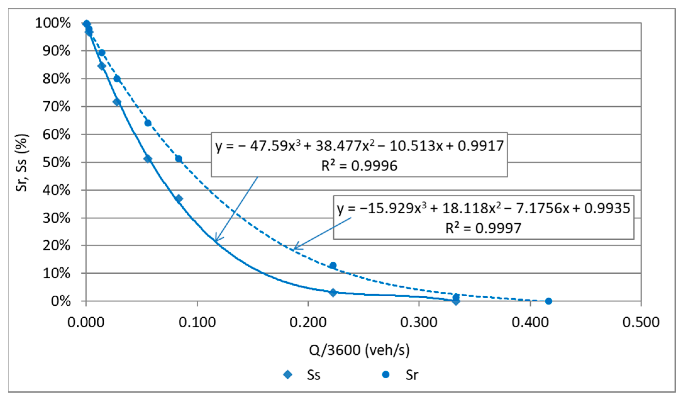
Figure 16 shows the curves
and
for
veh/h interpolated, assuming the values in
Table 1, using third-degree polynomials, to be used for the calculation of the probability
, which are expressed as follows:
The modified daily trends are shown in
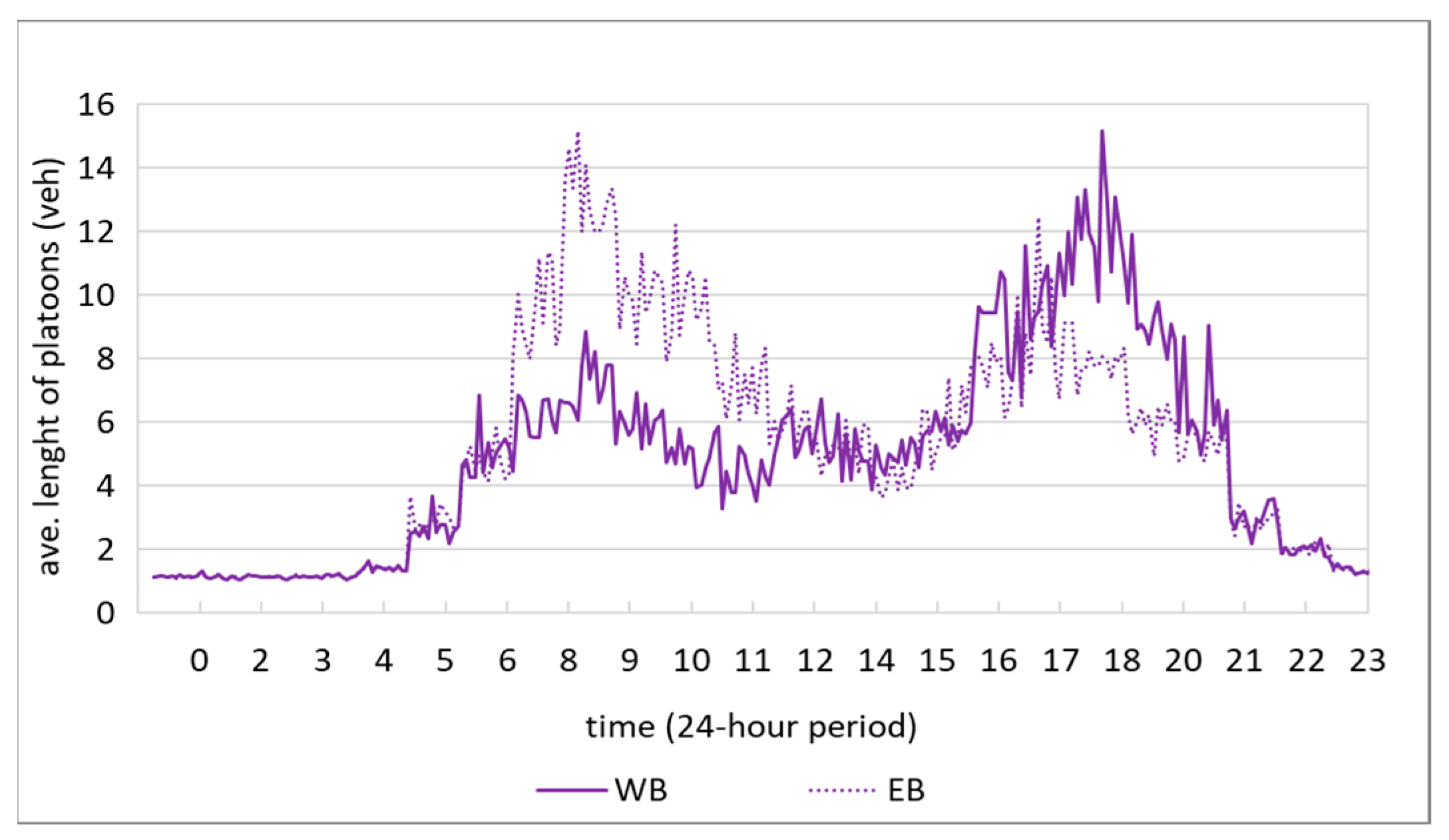
Figure 17, highlighting how the overtaking possibility allows for lower no-free vehicle rates in the hours with lower traffic, as was previously qualitatively supposed. It is possible to evaluate the average length of the platoon in intervals of 5 min, obtaining the daily trends shown in
Figure 18. Comparing
Figure 15 and
Figure 18, we can see how the absence of the no-overtaking rule lowers the average length of the platoon during the night period, bringing it below two vehicle units.
7. Conclusions
This paper presents a computational procedure that allows for evaluating the average percentage of vehicles free to travel at the desired speed and of non-free vehicles constrained to travel at lower speeds than desired as a function of the traffic flow on a two-lane road. The TLR-SPM constitutes an improvement of a method in literature by [
27,
32], with a more general approach deriving from the removal of the assumptions of normal distribution of the actual speeds and constancy of the means and variances of the same, relating to the variable time headways.
Without hypothesizing, identifying, and estimating the probability laws for speed and time headway, such as in probabilistic mixed-type models, the TLR-SP Model bases its computing on the average link between the vehicle speeds of the traffic flow through the determination of their covariance as a function of the time headway. In this way, it is possible to obtain more precise information with respect to applying the widespread criterion of the 3 s threshold, which does not consider vehicles that can be free (or not free) to travel at their desired speed while traveling over smaller (or greater) distances.
In particular, the proposed TLR-SP Model:
Allows us to overcome the approach that we find in a part of the technical literature, which sets a deterministic headway threshold for the distinction between free and non-free vehicles;
Decouples analyses from the specification of certain probabilistic distributions for the headways and the estimation of the related parameters that we can find in research works more focused on the probabilistic modeling aspects;
Constitutes an improvement of a method in the literature by [
27,
32], with a more general approach deriving from the removal of the assumptions of the normal distribution of the actual speeds and constancy of the means and variances of the same;
Achieves greater adaptability to experimental data due to its data-driven approach based on behaviors that emerge statistically from real-life, compared to other models in the literature;
Provides an agile but not simplistic method for evaluations in technical applications related to traffic quality assessment on two-lane roads;
Offers helpful support for two-lane road operating conditions improvement to promote their safety and efficiency as part of a sustainable transport system.
The explicative application to the case study of the two-lane road in Northern Italy also helps to specify the overall effects on the level of service, linked to the road section geometry and the driving rules, especially concerning the no-overtaking rule.
The results show how, with a more in-depth approach than the threshold value suggested by the HCM, but without hypotheses on the distribution of progress and speeds, it is possible to analyze the phenomena of interest with a data-driven approach based on some statistics and some interpolation. It is evident that, although the results of the case study may not have general validity because they refer to a specific section where there is a speed limit of 90 km/h, a rule prohibiting the passage of heavy vehicles over 3.5 tons, and a no-overtaking rule for all vehicle categories, the generalized model has no restrictions in its application. From this point of view, further investigations will be addressed through continuing the research on TLR-SPM. These will concern interesting insights about the presence of other vehicular categories, such as heavy-duty (HD) and connected automated vehicles (CAV) [
9,
10,
11] in the “smart road” context [
41], and the influence of local fluctuations in traffic parameters extended to different geometric characteristics and road regulations than those examined here, with comparisons, sensitivity analyses, and the application of other alternative methods.


