Spatiotemporal Variation of Groundwater Extraction Intensity Based on Geostatistics—Set Pair Analysis in Daxing District of Beijing, China

Abstract

In this paper, the authors studied the impact of human activities on the groundwater environment to reduce the impacts such activities for sustainable groundwater use. The authors took the monthly water table depth data of 32 long-term observation wells in the Daxing District of Beijing from 1986 to 2016 as samples. The authors used seven interpolation methods in the statistics module of ArcGIS by comparing the average error (ME) and root mean square error (RMSE) between the measured and predicted values so that the authors can select the best interpolation method. Using the geostatistical variogram model variation, the authors analyzed the nugget effect through time in the study area. On the basis of the set pair analysis, the main factors causing the increase in groundwater exploitation intensity were quantitatively evaluated and identified. The results were as follows. (1) After comparing the simulation accuracy of the seven interpolation methods for water table depth, ordinary Kriging interpolation was selected as the best interpolation model for the study area. (2) The spatial correlation of the water table depth gradually weakened, and the nugget effect from 2006 to 2016 was 25.92% (>25%). The data indicated that human groundwater exploitation activities from 2006 to 2016 greatly influenced the spatial correlation of the water table depth. (3) The average mining intensity of groundwater from 2006 to 2016 was medium (Level II), and a bleak gradual deterioration trend was observed. The evaluation results of the subtraction set pair potentials in 2010 and 2013, the years of key regulation of groundwater exploitation intensity, are partial negative potential and negative potential, respectively. In 2010, three indicators had partial negative potential: industrial product, tertiary industry product, and irrigated field area. In 2013, five indicators were in negative potential: irrigated area, vegetable area, facility agricultural area, fruit tree area, and the number of wells. Herein, the spatial and temporal variations in the water table depth of the study area are analyzed using a geostatistical method. Moreover, the influence of each water part on the groundwater exploitation intensity is further diagnosed and evaluated based on set pair analysis. The obtained results can provide a theoretical and methodological reference for the sustainable utilization of groundwater in regions where groundwater is the main water supply source, providing a basis for industrial regulation policies in the region.

1. Introduction

As an important freshwater resource, groundwater is significant for urban life and industrial and agricultural production. Especially in areas lacking surface water, groundwater may be the only stable water supply source. In Beijing, a city located north of North China Plain, the average annual rainfall is 585 mm. Its average water resource is 165 m³ per capita, accounting for approximately 8% of China’s water resources per capita. Moreover, Beijing is located in a semiarid and semihumid region affected by a continental monsoon climate, and the uncertainty of groundwater exploitable volume increases. These reflect the dire water resources situation in Beijing. In addition, rapid urbanization in the past 20 years has changed the original natural underlying surface and, consequently, the groundwater recharge and discharge processes. It has caused environmental problems, such as the continuous water table depth decrease in regional groundwater, settling of the ground surface, and deterioration of water quality. Even with the South-to-North Water Diversion Project in Beijing, groundwater still covers a significant proportion of the city’s water supply. The exploitable amount of groundwater resources refers to the maximum amount of water that can be obtained from the aquifer without causing deterioration of the ecological environment, which is mainly related to the recharge and consumption of groundwater. According to the relevant research results from 1989 to 2000 [1], the average annual recharge of groundwater in the Beijing plain area was 27.66 × 10⁸ m³/a, in which rainfall infiltration accounted for 47.92%, lateral recharge in mountainous areas accounted for 24.74%, irrigation recharge accounted for 12.86%, and canal infiltration recharge accounted for 14.48%. More than 92% of the lateral supply in mountainous areas comes from the atmospheric precipitation. Furthermore, atmospheric precipitation accounts for a large proportion of groundwater recharge. According to the Beijing Water Resources Bulletin, the average rainfall in Beijing from 2006 to 2019 was 549.86 mm, and from 1989 to 2000 was 549.92 mm, a minute difference indicating that the overall change in groundwater recharge was not considerable. The average annual groundwater consumption in Beijing plain from 1989 to 2000 was 30.27 × 10⁸ m³/a, in which groundwater exploitation accounted for 87.64%. The artificial exploitation of groundwater has an absolute advantage over the consumption of groundwater. Therefore, studying the spatiotemporal variability of groundwater exploitation intensity is of great practical significance and theoretical value for reducing the impact of human activities on the groundwater environment and realizing the sustainable utilization of groundwater.

Changes in water table depth significantly correlate with groundwater exploitation intensity [2,3,4]. Thus, these can reflect the intensity of groundwater extraction in a region by collecting water table depth data from monitoring wells at the water level and establishing a correlation model. However, because water table data around monitoring wells are limited, the authors should choose a spatial interpolation model with the slightest error if the authors must characterize the spatial variation of the water table depth in the whole region. Deterministic and geostatistical interpolation methods are commonly used for this purpose [5,6,7,8,9]. On the basis of similarity or smoothness within the study area, deterministic interpolation methods create surfaces using known points [10,11]. The deterministic interpolation methods can be divided into two types: global and local. Global interpolation methods use the sample data set of a whole study area to calculate predictive values (e.g., global polynomial interpolation [GPI]). In contrast, local interpolation methods use known sample points within a small spatial area of a large study area to calculate predictive values (e.g., inverse distance interpolation [IDW], radial basis interpolation, and local polynomial interpolation [LPI]). Geostatistical interpolation methods mainly include ordinary Kriging interpolation (OK), simple Kriging interpolation (SK), pan-Kriging interpolation, probabilistic Kriging interpolation, disjunctive Kriging interpolation, and collaborative Kriging interpolation. These methods are based on the theory of variation function and structural analysis. These methods are used for the optimal unbiased estimation of regionalized variables in limited regions [12,13].

As a unique function of geostatistical analysis, semi-variation is a quantitative expression of the theorem of close geographic resemblance [14,15]. The strength of the geographical spatial correlation can be reflected by the nugget effect (nugget/sill). The larger the nugget effect, the greater the variation between samples caused by random factors [16,17]. Structural factors can enhance the spatial correlation of the water table depth, such as precipitation, topographic undulations, and water-containing rocks. Contrarily, human exploitation belongs to stochastic factors, which weaken the spatial correlation.

Although the nugget effect can identify the spatial variability of water table depth over time, further diagnosing and evaluating the main factors affecting groundwater exploitation is necessary for controlling it. Some evaluation methods are used in developing and utilizing groundwater. These include the water balance method [18,19], numerical simulation method [20,21], isotope tracer method [22], principal component analysis, fuzzy comprehensive analysis, risk matrix method, projection pursuit method [23], and set pair analysis method [24,25]. Among these, set pair analysis can reflect the uncertainty relationship between evaluation indexes and evaluation standards from the three aspects of identity, difference, and opposition. Thus, it has unique advantages for treating water resources systems. The adjoint functions of set pair analysis include subtraction set pair potential [26], a partial linkage coefficient [27], and a neighbor-joining coefficient [28].

To reduce the impact of human activities on groundwater environment for the sustainable utilization of groundwater, in this study, the Daxing District in Beijing is used as the research area, and the best interpolation model is selected from the seven interpolation methods in the ArcGIS statistics module. The spatial variability characteristics of groundwater depth are analyzed using the geostatistical function model. The main source of water supply in the study area is groundwater, and the types of water use mainly include agricultural water, industrial water, tertiary industry water and domestic water. Therefore, this paper uses the agricultural irrigation area, industrial output value, tertiary industry output value, population, and the number of wells as the evaluation indexes. Using set pair analysis, the authors quantitatively evaluated and identified the main factors causing the increase in groundwater exploitation intensity. The research results can provide a theoretical and methodological reference for the sustainable utilization of groundwater in areas where groundwater is the main source of water supply, providing a basis for industrial regulation policies in the region.

2. Materials and Methods

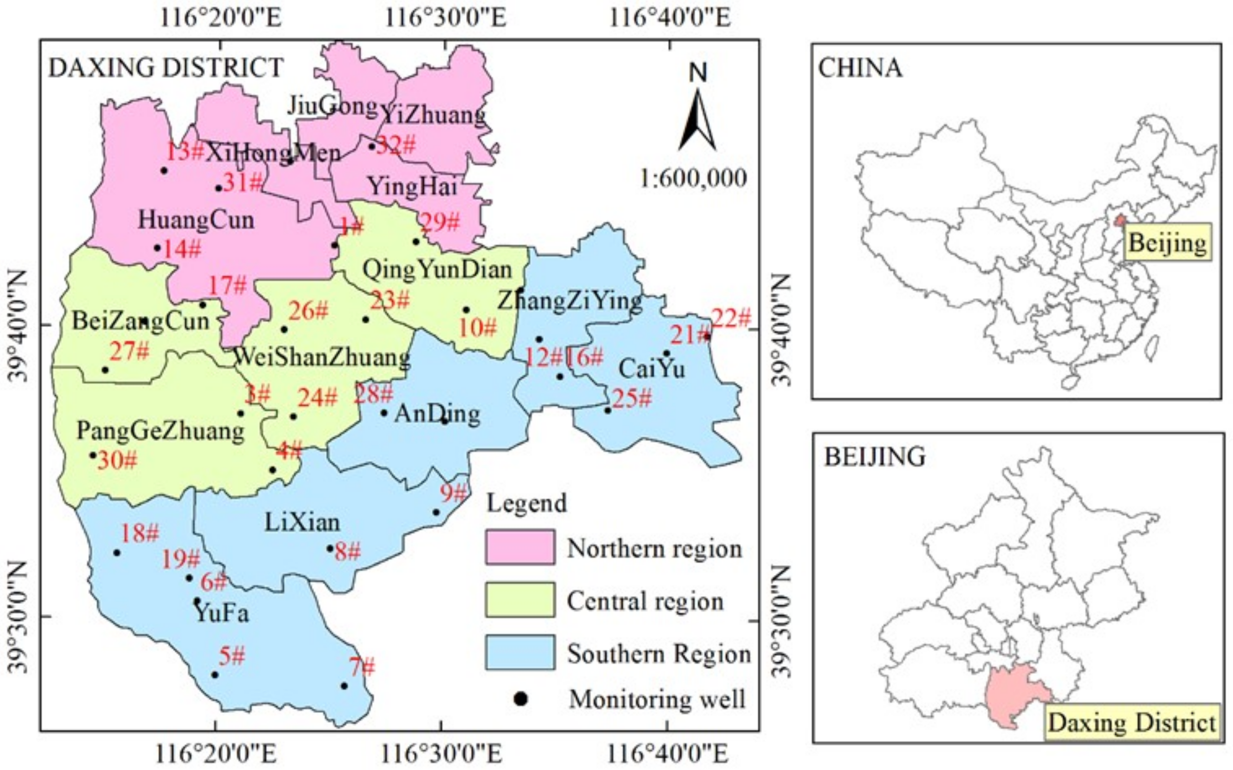
2.1. Study Area

The Daxing District is located in the southern plains of Beijing (39°26′–39°51′ N, 116°13′–116°43′ E). It has 14 townships and an area of approximately 1036 km². It has a warm, temperate, semihumid, semiarid continental monsoon climate with well-defined seasons: cold and less rainy in winter and spring, hot and rainy in summer, and comfortable in autumn. The average annual rainfall is 510.1 mm, with large annual and interannual rainfall distributions. The annual average temperature is 11.7 °C, and the maximum frozen soil depth is 69 cm. The Daxing District belongs to the Yongding River floodplain, which has a flat topography elevated from 9 to 73 m and a topographic slope of about 0.5–2.0‰. The soil type is predominantly sandy loam with a coarsening gradient from west to east. The Daxing District is an important strategic node for the Beijing–Tianjin–Hebei coordinated development. It has four primary industries: metropolitan industry, modern service industry, cultural creative industry, and urban modern agriculture. With the construction of the Beijing Daxing International Airport, the Daxing District is slated to become one of the fastest-growing regions in Beijing.

2.2. Data Sources

2.2.1. Groundwater Water Level Data

Long-term monthly water table depth monitoring data from 32 observational logs in the study area from 1986 to 2016 were collected to monitor the dynamics of water table depth. The monitored well locations are shown in Figure 1.

2.2.2. Statistical Information

The annual statistical data used in this paper were collected from relevant data, including the Beijing water service statistical yearbook from 2012 to 2017, the Daxing District statistical yearbook from 2005 to 2017, the groundwater harvest well census results of the Beijing census of water services from 2013, and the third agricultural census data compilation from the Daxing District of Beijing in 2016.

2.3. Research Method

2.3.1. Error Calculation Methods for the Interpolation Model

In this paper, seven methods are used to model the groundwater water level: IDW, GPI, LPI, tension spline interpolation (Tspline), OK, SK, and the universal Kriging method (UK). The advantages and disadvantages of each interpolation method are shown in

Table 1. Advantages and disadvantages of each interpolation method.

Method	Advantages	Disadvantages
IDW	Wide application range and fast calculation speed	IDW can produce bullseyes around data
GPI	Suitable for surface with slow change in spatial data and fast calculation speed	The edge position of data has great influence on the interpolation result
LPI	Suitable for reflecting short-range change of spatial data and medium computing speed	Prone to strip phenomenon
Tspline	Suitable for surfaces with flat spatial data. Compared with GPI, this method provides accurate interpolation and has medium calculation speed	In a short range, when the data change considerably or the sampling point data have great uncertainty, the interpolation results will be greatly affected
OK	The interpolation accuracy is less affected by the sample density and number, and the interpolation effect is good with high accuracy	Intensive calculation and slow operation speed
SK	SK is the same as OK, but also the linear estimation of regionalized variables; the interpolation effect is slightly worse than OK	Intensive calculation and slow operation speed
UK	UK is an extension of OK, which can add explanatory variables to the model	Intensive calculation and slow operation speed

. The average errors (MEs), root mean square errors (RMSEs), and Nash–Sutcliffe efficiency coefficient (NSE) of the different methods are compared to select the best model.

The mean square error, root mean square error, and Nash–Sutcliffe efficiency coefficient (NSE) are calculated as follows:

• The mean square error

  $$\mathrm{ME}=\frac{1}{n}{\displaystyle \sum _{i=1}^n\left|z^{*}\left(p_i\right)-z\left(p_i\right)\right|}$$

  (1)
• Root mean square error

  $$\mathrm{RMSE}=\sqrt{\frac{1}{n}{\displaystyle \sum }_{i=1}^n{\left|z^{*}\left(p_i\right)-z\left(p_i\right)\right|}^2}$$

  (2)
• Nash–Sutcliffe efficiency coefficient

  $$\mathrm{NSE}=1-\frac{{\displaystyle \sum _{i=1}^n{(Z^{*}(p_i)-Z(p_i))}^2}}{{\displaystyle \sum _{i=1}^n{(Z^{*}(p_i)-\overline{Z^{*}})}^2}}$$

  (3)

In these equations, ME represents the mean error, RMSE is the root mean square error, NSE represents the Nash–Sutcliffe efficiency coefficient, n represents the sample size, Z(P_i) is the measured value for position P_i, Z*(P_i) is the predicted value for position P_i, and $\overline{Z^{*}}$ is the total average of measured values. According to formula (1), formula (2), and formula (3), the average error (ME), root mean square error (RMSE), and Nash–Sutcliffe efficiency coefficient (NSE) of seven interpolation methods were compared. The interpolation method with the smallest ME and RMSE and the closest NSE to one was selected as the best interpolation method.

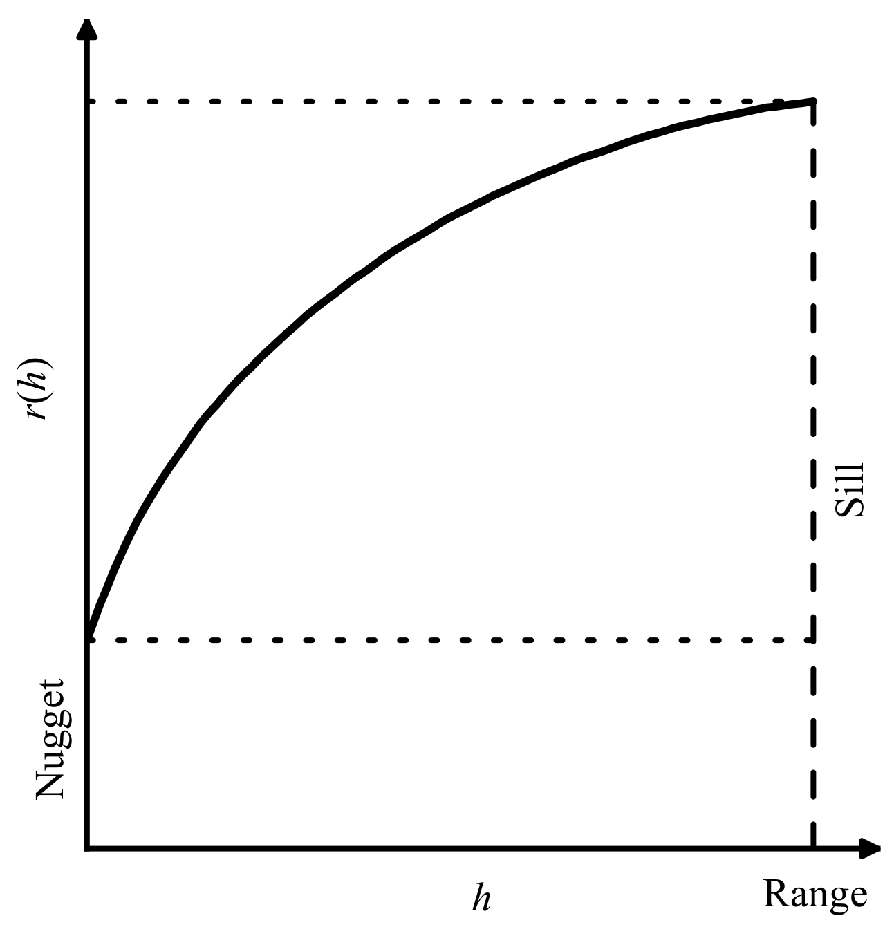
2.3.2. Calculating the Nugget Effect

The semi-variation coefficient expresses the geographic proximity of similarly quantified expressions [14].

Figure A1 shows that the semi-variation value r(h) increases with distance h because the semi-variation function manifests the spatial correlation coefficient of things. These things are more similar when they are closer to each other and have smaller half mutation values. At greater distances, their similarity weakens, and the half mutation value increases.

When the sampling site distance is 0, the semi-variation function value should be 0. However, when two sampling sites are so close because of measurement error and spatial variation, the semi-variation function value is not 0; that is, these sites form a nugget. The abutment value is when the sampling point increases with the distance h and the semi-variation function r(h) reaches a relatively stable constant from the initial nugget value, called the sill. The spatial correlation does not exist when the variant function value exceeds the abutment value; that is, the functional value does not change with the sampling site interval distance. The variable range is the interval distance between sampling sites when the value of the semi-variation function is taken to reach the abutment value from an initial tuber value.

The nugget effect, which is the ratio of the nugget to the sill, characterizes the strong spatial correlation across samples. The smaller the nugget effect, the smaller the impact of artificial mining on water table depth, and the greater the spatial correlation of water table depth. The greater the nugget effect, the greater the influence of artificial mining on water table depth, and the smaller the spatial correlation of water table depth. A nugget effect <0.25 indicates that the variables are strongly influenced by natural structural factors and have strong spatial correlations. A nugget effect between 0.25 and 0.75 indicates that the variable is influenced by both natural structural and stochastic factors, and the spatial correlation is moderate. When the nugget effect is >0.75, the variables are greatly affected by stochastic factors and have a weak spatial correlation [29].

The nugget effect is calculated as

$$Nugget effect=\frac{Nugget}{Sill}$$

(4)

2.3.3. Evaluation and Diagnosis of Groundwater Exploitation Intensity Based on Set Pair Analysis

The connection number of set pair analysis is calculated, and the grade of exploitation intensity determined to establish the evaluation and diagnosis model of groundwater exploitation intensity. Then, subtraction sets are used to identify the main factors affecting the intensity of groundwater extraction. The main steps are as follows:

• Establishment of an evaluation index system and classification of regional groundwater extraction intensity

Because the local natural surface water resources in the study area are insufficient, have low water quality, and cannot be used directly as a water supply, the regional water supply is mainly groundwater and regenerated water. Groundwater composes about 70% of the total water supply. Regenerated water is primarily used for ecological river use, accounting for about 30%. The types of water used in the study area mainly include agricultural water, industrial water, tertiary industry water, domestic water, and ecological water. Agricultural water is used mainly in grain fields, gardens, facility agriculture, and fruit tree irrigation, and the irrigation area of each type is taken as an evaluation indicator. The industrial output is taken as an industrial water evaluation indicator. The tertiary industry output is taken as a tertiary industry water evaluation indicator. The population number is taken as a domestic water evaluation indicator. In addition, the number of wells in the study area is used as a groundwater mining index of groundwater extraction intensity. Therefore, considering practicality, hierarchy, and operability [30], an evaluation index system for evaluating the intensity of groundwater extraction in the township and town areas of the Daxing District and jurisdiction is constructed in this paper. The evaluation indicators of this system are the population (10,000 people), total industrial output (100 million yuan), tertiary industry output (100 million yuan), irrigated area (10,000 mu), vegetable area (10,000 mu), facility agriculture area (10,000 mu), fruit tree area (10,000 mu), and number of machine wells (10,000 eyes).

By referring to the results of previous studies [31] and comprehensively considering economic, social, ecological, and other factors and expert opinions, the intensity of groundwater extraction is classified into three levels, namely, Levels 1, 2, and 3, representing “weak,” “medium,” and “strong” groundwater extraction intensity, respectively.

2.

Calculation of connection numbers for evaluation samples

Equation (5) is used to calculate the connection number of evaluation samples. u_1i represents the number of ternary contacts of sample i. n_a, n_b, and n_c indicate the number of evaluation indicators of sample i that are in Levels 1, 2, and 3, respectively. w_j is the weight value of the jth indicator. a₁, b₁, and c₁ respectively denote the sample set pair degrees of identity, divergence, and antagonism, and their values are v_1i1, v_1i2, and v_1i3, respectively. I and J denote the coefficient of difference and the coefficient of opposition, respectively.

$$u_{1i}={\displaystyle \sum _{j=1}^{n_a}{w}_j+{\displaystyle \sum _{j=n_a+1}^{n_a+n_b}{w}_{j}I+{\displaystyle \sum _{j=n_a+n_b+1}^{n_a+n_b+n_c}{w}_j}}}J=v_{1i1}+v_{1i2}I+v_{1i3}J=a_1+b_{1}I+c_{1}J$$

(5)

3.

Calculation of the connection number of the evaluation index

The number of contact u_2ijk of the evaluation index must be calculated to represent the affiliation degree between the evaluation index x_ij and the evaluation standard S_kj, where i is the ith sample, j represents the jth indicator, and k represents the rank number.

If the evaluation index is a positive indicator and S_0j < x_ij ≤ S_1j or it is a reverse indicator and S_0j > x_ij ≥ S_1j, the index contact number is calculated using equation (6):

$$\left\{\begin{array}{l}{u}_{2ij1}=1\\ u_{2ij2}=1-\frac{2\left(S_{1j}-x_{ij}\right)}{\left(S_{1j}-x{i}_j\right)}\\ u_{2ij3}=-1\end{array}\right.$$

(6)

If the evaluation index is a forward indicator and S_1j < x_ij ≤ S_2j or it is a reverse indicator and S_1j > x_ij ≥ S_2j, the index contact number is calculated using Equation (7):

$$\left\{\begin{array}{l}{u}_{2ij1}=1-\frac{2\left(x_{ij}-S_{1j}\right)}{S_{2j}-S_{1j}}\\ u_{2ij2}=1\\ u_{2ij3}=1-\frac{2\left(S_{2j}-x_{ij}\right)}{S_{2j}-S_{1j}}\end{array}\right.$$

(7)

If the evaluation index is a forward indicator and S_2j < x_ij ≤ S_3j or it is a reverse indicator and S_2j > x_ij ≥ S_3j, the index contact number is calculated using Equation (8):

$$\left\{\begin{array}{l}{u}_{2ij1}=-1\\ u_{2ij2}=1-\frac{2\left(x_{ij}-S_{2j}\right)}{S_{3j}-S_{2j}}\\ u_{2ij3}=1\end{array}\right.$$

(8)

A forward indicator occurs when the rank value increases with the index value; otherwise, it is a reverse indicator. S_0j, S_1j, S_2j, and S_3j are the minimum, critical value of Levels 1 and 2, critical value of Levels 2 and 3, and maximum value of index j, respectively.

The degree of membership between the contact number of sample indicators and the evaluation criteria can be expressed as follows:

$$v_{2ijk}^{*}=0.5+0.5u_{2ijk}$$

(9)

In calculating the contact number of sample indicators u₂, Equation (9) is first normalized, and the calculation formula is as follows:

$$v_{2ijk}=\frac{v_{2ijk}^{*}}{{\displaystyle \sum _{k=1}^3{v}_{2ijk}^{*}}}$$

(10)

$$u_{2i}={\displaystyle \sum _{j=1}^{n_a}{w}_j{v}_{2ij1}+{\displaystyle \sum _{j=n_a+1}^{n_a+n_b}{w}_j{v}_{2ij2}I+{\displaystyle \sum _{j=n_a+n_b+1}^{n_a+n_b+n_c}{w}_j}}}{v}_{2ij3}J=v_{2i1}+v_{2i2}I+v_{2i3}J=a_2+b_{2}I+c_{2}J$$

(11)

In the formula, v_2ijk represents the contact number component of the jth indicator in the ith sample. u_2i indicates the contact number of sample indicators i. a₂, b₂, and c₂ respectively represent the sample index set pairs’ degree of identity, divergence, and antagonism, and their values are v_2i1, v_2i2, and v_2i3, respectively.

4.

Calculation of average contact number

The average contact number by sample is obtained by taking the contact number of a sample and the contact number of an index to sufficiently extract sample information [26]:

$$v_{ik}=\frac{{\left(v_{1ik}{v}_{2ik}\right)}^{0.5}}{{\displaystyle \sum _{k=1}^3{\left(v_{1ik}{v}_{2ik}\right)}^{0.5}}}$$

(12)

$$u_i=v_{i1}+v_{i2}I+v_{i3}J$$

(13)

In the formula, v_ik represents the mean number of contact components of the ith sample. u_i indicates the average number of contacts for the ith sample.

5.

Determination of the intensity levels of underground extraction

The values of groundwater extraction intensity between sample i and index j are calculated separately using the level eigenvalue method [32], and the calculations are as follows:

$$h\left(i\right)={\displaystyle \sum _{k=1}^3{v}_{ik}k}$$

(14)

$$h\left(j\right)={\displaystyle \sum _{k=1}^3{v}_{2ijk}k}$$

(15)

In the formula, h(i) represents the value of groundwater extraction intensity for the ith sample, and h(j) represents the groundwater extraction intensity value of the jth indicator.

6.

Diagnosis of groundwater extraction intensity based on the number of linkages

The identification of key indicators affecting the intensity of groundwater extraction uses subtraction set pair potentials [26].

According to the set pair analysis theory, the subtraction set pair potential for the number of contacts essentially reflects the relative ascertainment status and developmental trends of the study subjects. The subtraction set pair potential S_f(u) is defined as

$$s_f\left(u\right)=a-c+ba-bc=\left(a-c\right)\left(1+b\right)$$

(16)

In the formula, s_f(u) ∈ [−1, 1]. According to the principle of uniformity, the subtraction set pair potentials can be divided into five grades: negative potential, s_f(u) ∈ [−1, −0.6); partial negative potential, s_f(u) ∈ [−0.6, −0.2); balanced potential, s_f(u) ∈ [−0.2, 0.2]; partial positive potential, s_f(u) ∈ (0.2, 0.6]; and positive potential, s_f(u) ∈ (0.6, 1.0]. Positive and partial positive potentials illustrate that research subjects favorably develop. Negative and partial negative potentials illustrate that research subjects develop in an unfavorable direction and thus require focusing on and regulating indicators of these negative states. The homogeneous potential is an uncertain state.

The total adjacent subtraction is obtained by calculating the difference between the degree of identity a and the degree of difference b, degree of opposition c, and degree of difference b, which reflects developmental changes of things [33]. The specific calculation procedure is as follows:

$$u_3=\left(a-c\right)+\left(b-c\right)\left(a-b\right)+\left(b-a\right)\left(c-b\right)$$

(17)

In the formula, u₃ ∈ [−2, 1.0625], where, when a = 0, b = 1, and c = 0, u_3min = −2; when a = b = 0, c = 1, and c = 1, u₃ = −1; when a = 0.875, b = 0.125, and c = 0, u_3max = 1.0625. When u₃ changed from −2 to 1.0625, the trend of the research object gradually changes from inverse potential to potential, but the critical state cannot be determined.

The potential function can also judge the trend of the set toward the development of events. Its value is also larger, indicating that the research subjects move toward the same potential [28]. The specific calculation is as follows:

$$Shi\left(u_4\right)=\left(\raisebox{1ex}{$a$}\!\left/ \!\raisebox{-1ex}{$b$}\right.\right)/\left(\raisebox{1ex}{$b$}\!\left/ \!\raisebox{-1ex}{$c$}\right.\right)=ac/b^2$$

(18)

3. Results and Discussion

3.1. Results of the Interpolation Calculation of Water Table Depth

The parameters selected for each interpolation method to obtain the spatial distribution characteristics of water table depth in the study area should have minimal errors. The selection of model parameters and error accuracy is shown in

Table 2. Interpolation model parameters and interpolation error table of water table depth from 1986 to 2016.

Interpolation Model	Data Conversion	Maximum Number of Predicted Points within the Search Radius	Minimum Number of Predicted Points within the Search Radius	Variation Function	Mean (m)	Root Mean Square (m)	Nash-Sutcliffe Efficiency Coefficient
IDW	no	15	10	/	0.1816	4.5373	0.70
GPI	no	/	/	/	0.0787	5.2072	0.81
LPI	no	20	10	/	0.1309	3.9898	0.83
Tspline	no	25	10	/	0.1348	4.2010	0.80
OK	no	15	5	Globular model	0.0507	3.9577	0.89
SK	no	16	5	Gaussian model	0.0517	4.0492	0.86
UK	no	12	5	Globular model	0.0536	3.9865	0.88

.

Table 2 shows the deterministic interpolation method is less accurate than the geodesic statistical interpolation method. Among all listed methods, IDW has the largest error and a poor interpolation effect, which may be due to the existence of some extreme points in the interpolation process [5,15]. Tspline, similar to IDW, is susceptible to the influence of extreme value points [7,17], resulting in less effective interpolation, as shown by its ME and RMSE. LPI, which is suitable for local spatial interpolation, shows high simulation accuracy for short-range variations [7,11]. However, it predicts a large fluctuation of results for the analysis of 30 older sequences in the water table depth; thus, its interpolation accuracy is low. GPI is based on the sample data as a whole [5,7,14]. The higher the number of interpolations, the better the interpolation effect. However, the complexity and error are also relatively increased. This high number of interpolations also results in the largest RMSE and a poor prediction effect.

The ME of OK, SK, and UK differ minimally, but the RMSE of the OK method is less than those of SK and UK. Furthermore, the NSE of the geostatistical interpolation method is closer to 1 than that of the deterministic interpolation method, indicating that the geostatistical method is more reliable than the deterministic interpolation method. Among the geostatistical interpolation methods, the NSE of the OK is higher than that of SK and UK, indicating that OK has the highest reliability. Thus, the best interpolation method selected is the OK method.

3.2. The Spatial-Temporal Distribution Rules of Water Table Depth

The water table depth in 1986, 1996, 2006, and 2016 is spatially interpolated using the OK method.

Figure 2 shows that the overall water table depth in the Daxing region constantly decreased. From 1986 to 2016, the water table depth of the regional subsurface decreased from 8.1 to 17.60 m, with an average annual decline rate of 0.30 m. From 1986 to 1996, the water table depth decreased from 8.1 to 10.80 m, with an average annual decline of 0.27 m. From 1996 to 2006, the water table depth decreased from 10.80 to 17.34 m, with an average annual decline of 0.65 m. From 2006 to 2016, the water table depth decreased from 17.34 to 17.60 m, with an average annual decline rate of 0.03 m.

From the above analysis, the period with the most significant decline rate of water table depth in the Daxing District is from 1996 to 2006. This indicates that the groundwater in this period is in a state of overdraft, resulting in a continuous decline of water table depth. From 2006 to 2016, the water table depth was almost flat, although it decreased slightly. This indicates that groundwater is basically in the state of mining–compensation balance, which may be related to the extensive use of regenerated water locally. However, environmental and geological problems caused by groundwater overmining remained serious because of the previous continuous years of overdraft.

From 1986 to 2016, the decline rates of water table depth in the northern, central, and southern Daxing District are 0.23, 0.49, and 0.18 m/a, respectively. These indicate that the central region had the largest rate of water table depth decline, followed by the northern and southern regions. Groundwater depression funnels can be found in the Qingyundian and Beizangcun in the central region, with a continuous outward diffusion trend. Thus, groundwater exploitation control in the region should be strengthened. The deepest water table depth in the north is always higher than that in the middle and south, which may be related to population distribution and the industrial layout in the Daxing District. Compared with those in the northern and central regions, the water table depth and water table decline rate in the southern region are relatively small. However, from 1986 to 2006, the water table depth decreased from 6.04 to 11.82 m, and the water table depth continued to decline. Thus, the southern region is also in a state of continuous overextraction.

3.3. Spatial Variability Analysis of Groundwater Depth

In identifying the main factors causing the decline of water table depth, the nugget effects of the three periods from 1986 to 1995, 1996 to 2005, and 2006 to 2016 are calculated to analyze the spatial variability characteristics of water table depth using the OK method.

As shown in

Table 3. Semi-variogram model parameters of water table depth from 1986 to 2016.

Name	1986–1995	1996–2005	2006–2016
Nugget value	1.88	5.85	28.03
Partial sill	47.06	45.53	78.95
Sill	48.94	51.38	106.98
Nugget effect	0.04	0.10	0.26

, the nugget effect of water table depth increased from 1986 to 2016, indicating that its spatial correlation gradually weakened and that the influence of human activities on water table depth increased. The nugget effect increased from 0.04 to 0.10 in 1986–1995 and 1996–2005. Compared with that in 1996–2005, the nugget effect increased from 0.10 to 0.26 in 2006–2016 (greater than 0.25), indicating that human extraction activities have become an essential factor affecting water table depth. Therefore, further evaluating and diagnosing the existing groundwater exploitation intensity is necessary to reduce the influence of human mining activities on the water table depth.

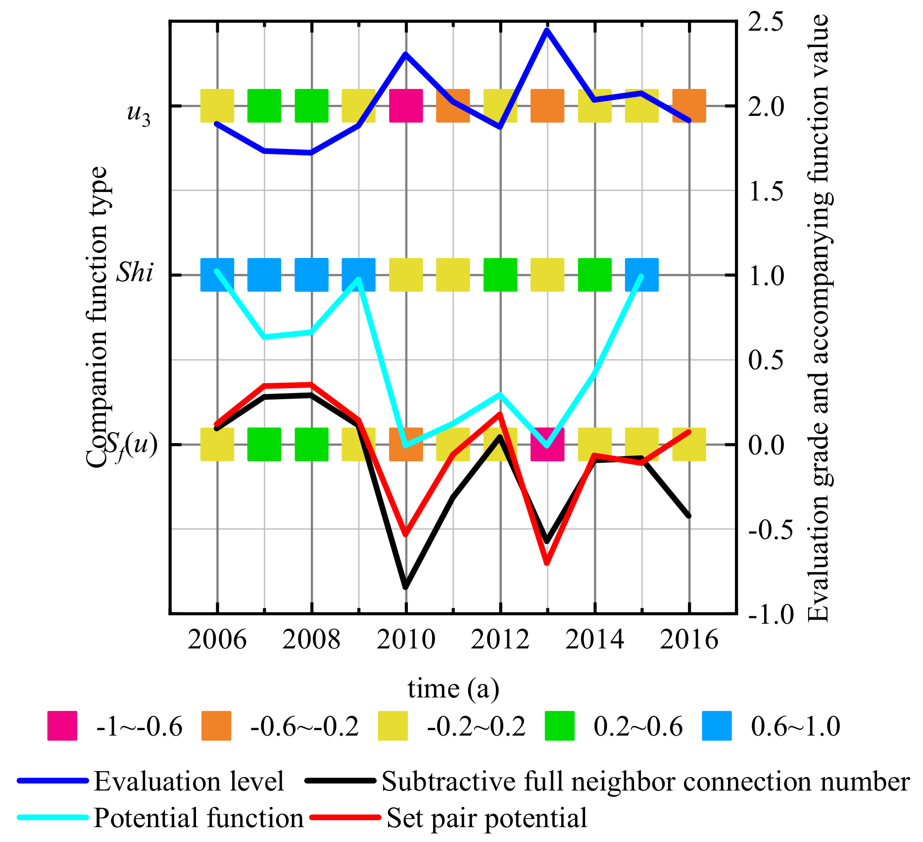
3.4. Determination of Groundwater Exploitation Intensity Levels and Identification of Key Control Years in the Daxing District Using Set Pair Analysis

An index system and an evaluation standard level of groundwater exploitation intensity in the Daxing District are determined according to the calculation method in Section 2.3.3 to analyze the spatiotemporal variation of groundwater exploitation intensity in the Daxing region from 2006 to 2016. The weight of each index is determined using the entropy weight–AHP method, as shown in

Table 4. Evaluation index, standard grade, and index weight of groundwater exploitation intensity in the Daxing District.

No.	Subsystem	Evaluation Index	Symbol	Evaluation Index			Index Weight
				Weak (Level I)	Medium (Level II)	Strong (Level III)
1	Domestic water	Population (10,000)	X1	≤115.90	115.90–150.70	>150.70	0.1480
2	Industrial water	Gross industrial production (100 million yuan)	X2	≤109.28	109.28–202.48	>202.48	0.1476
3	Tertiary industry water	GDP of the tertiary industry (100 million yuan)	X3	≤189.81	189.81–338.37	>338.37	0.1586
4	Agricultural water	Irrigation area (10,000 mu)	X4	≤18.42	18.42–19.35	>19.35	0.1132
5		Vegetable field area (10,000 mu)	X5	≤3.04	3.04–3.15	>3.15	0.1141
6		Facility agricultural area (10,000 mu)	X6	≤7.87	7.87–7.98	>7.98	0.0862
7		Fruit tree area (10,000 mu)	X7	≤6.96	6.96–31.33	>31.33	0.0565
8	Number of underground wells	Number of motorized wells (10,000 eyes)	X8	≤1.17	1.17–1.23	>1.23	0.1788

.

The subtraction set pair potential, total adjacent subtraction, and the potential function can all reflect the trend of event development. Thus, the potential function values and the total adjacent subtraction of each sample are calculated using Equations (18) and (17), respectively, to verify the rationality of the results of the subtraction set pair potential evaluation.

However, Equation (18) shows that the difference degree b of the potential function cannot be 0; when the difference degree is 0, the potential function method cannot judge the trend of event development. Equation (17) shows that the subtraction of all neighbors can judge the trend of an event. Still, it cannot judge the critical value of the situation where it is located. Fortunately, the subtraction set pair potential can deal with situations where the difference degree b is 0 and determines the critical value of the development trend of events. Therefore, it is selected for evaluating the potential of groundwater extraction intensity in this paper.

Figure 3 shows that the evaluation results using subtraction set pair potential, evaluation level, potential function, and subtractive full neighbor connection number are basically consistent. However, the evaluation level has a trend opposite to those of the other three methods. With greater development intensity, the evaluation level increased, whereas the other three methods decreased. Figure 3 shows that the groundwater development intensity is largest in 2013 in the Daxing District and smallest in 2008. The groundwater development intensity from 2006 to 2013 had an increasing trend year by year. However, it slightly eased from 2013 to 2016. The average connection number of groundwater development intensities for the whole region in 2010 and 2013 had partial negative potential and negative potential, respectively. In 2006, 2009, 2011–2012, and 2014–2016, they had balanced potential. In 2007–2008, they had partial positive potential. These were consistent with the results of the comprehensive review of the connection numbers. According to the evaluation results, the average mining intensity of groundwater in the Daxing District from 2006 to 2016 was medium (Level II) with a bleak gradual deterioration trend. The evaluation results of the subtraction set pair potential in 2010 and 2013 were partial negative potential and negative potential, respectively, and the comprehensive evaluation results were 2.31 and 2.45. The years 2010 and 2013 were the groundwater exploitation intensity key control years.

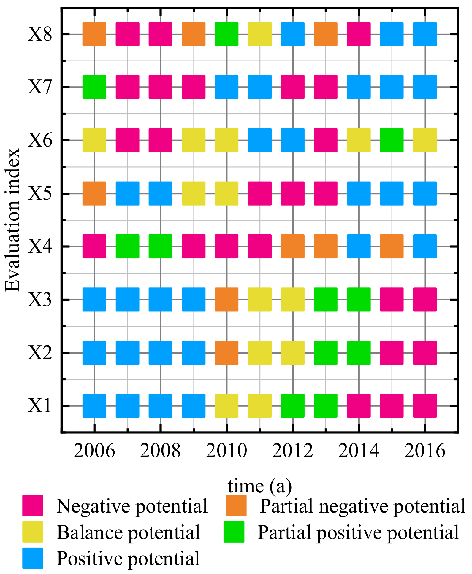
3.5. Identification of Main Factors Affecting Groundwater Exploitation Intensity in the Daxing District Based on Subtraction Set Pair Potential

The authors further identified the main factors affecting the intensity of groundwater extraction and provided technical support for groundwater management and protection. In this paper, the subtraction set of each evaluation index was used to diagnose and analyze the jth index of the ith evaluation sample, which can be obtained as the main index that caused the increase in groundwater extraction from 2006 to 2016 in the Daxing District. As shown in Figure 4, in 2010, three indicators had partial negative potential: industrial GDP, tertiary industry GDP, and irrigation area. In 2013, five indicators had negative potential: irrigated land area, vegetable field area, facility agriculture area, fruit tree area, and the number of wells. In Figs. 4 and 5, the trends of the subtracted set pair potential (evaluation level) of the gross industrial product (X2), gross tertiary industrial product (X3), and irrigation area (X4) are basically consistent between 2006 and 2016. However, the subtraction set pair potentials (evaluation grade) of these indicators significantly decreased (increased) in 2010, which may be related to the adjustment of the industrial structure in the Daxing District. The Daxing District began vigorous industrial and tertiary industrial developments from 2009 to 2010. Its industrial and tertiary industry output values in 2010 increased by 16.12% and 17.54%, respectively, compared with those in 2009. This rapid development resulted in the rapid increase of industrial water and tertiary industry water consumption.

The subtraction set pair potential (evaluation rank) of vegetable area (X5) from 2006 to 2016 had a continued decreasing (rising) trend from 2008 to 2013 (Figure 5). These indicate that the vegetable area (X5) had an increasing trend at this stage, leading to increased water consumption. The subtraction set pair potential (evaluation rank) of the facility agricultural area (X6) continued to increase (decrease) from 2008 to 2012, indicating that it had a decreasing trend at this stage. In 2013, the subtraction set pair potential appeared to increase, indicating that facility agricultural area (X6) had an increasing trend compared with that in 2012. The subtraction set pair potential (evaluation rank) of the fruit tree area (X7) had an increasing (decreasing) trend from 2008 to 2011 and a decreasing (increasing) trend from 2011 to 2013, indicating that it had an increasing trend in 2011–2013 compared with that in the previous stage. From these analyses and from Figs. 2 and 3, the authors can observe that the use of agricultural water has continuously decreased since 2014, which is considerably related to the implementation of agricultural water policies in Beijing. This indicates that the Daxing region has achieved good results in its water-saving social construction practice. The subtraction set pair potential (evaluation grade) of the number of wells (X8) showed an increasing (decreasing) trend from 2008 to 2012 and a decreasing (increasing) trend from 2012 to 2014. This indicates that the number of wells (X8) had a decreasing trend from 2008 to 2012, an increasing trend from 2012 to 2014, and a decreasing trend since 2014. The initial increasing and the ensuing decreasing trends for the number of wells (X8) indicate rapid population growth and the development of three major industries from 2008 to 2014, which continuously increased the demand for groundwater. Conversely, the number of opportunistic wells (X8) tended to decrease since 2014, which may be related to the water-affecting evaluation and approval system implemented in Beijing city and the rigor of new water use. It may additionally be related to the substitution of some subsurface water sources after the north-to-south water diversion into Beijing.

3.6. Research Implications and Limitations

The above analysis shows that from 1986 to 2016, the water table depth of the study area has been continuously declining as a whole, indicating that groundwater is in a state of continuous overexploitation and the impact of human exploitation on water table depth is increasing. Through set pair analysis, the main factors causing the increase in the groundwater exploitation intensity were further diagnosed and identified, showing that the groundwater exploitation intensity in this area had a bleak, gradual deterioration trend. The proposed research method can provide a method and theoretical reference for the sustainable utilization of groundwater in the region where the groundwater is the main source of water supply, providing a basis for the industrial regulation policy in this region. However, there are still some limitations in this paper, such as groundwater quality problems caused by the decline in the water table depth. Moreover, the best interpolation method selected in this paper may only be suitable for this area. Therefore, when performing spatial interpolation in other areas, the actual situation must be considered to reselect the optimal method.

4. Conclusions

The spatial variability of groundwater table depth in the study area is combined with the evaluation and diagnosis of groundwater exploitation intensity in this paper. The authors studied the impact of human extraction activities on the water table burial depth and identified the main factors affecting the groundwater extraction intensity. This research can provide theoretical support for sustainable groundwater use and industrial regulation policies in areas with water shortages. The conclusions are as follows:

• The OK method is selected as the best interpolation model after comparing the prediction accuracies of seven interpolation methods for the water table burial depth in the study area. The OK method had significantly higher accuracy than those of SK and UK. Its ME did not differ much from those of the other methods, but it had a significantly smaller RMSE.
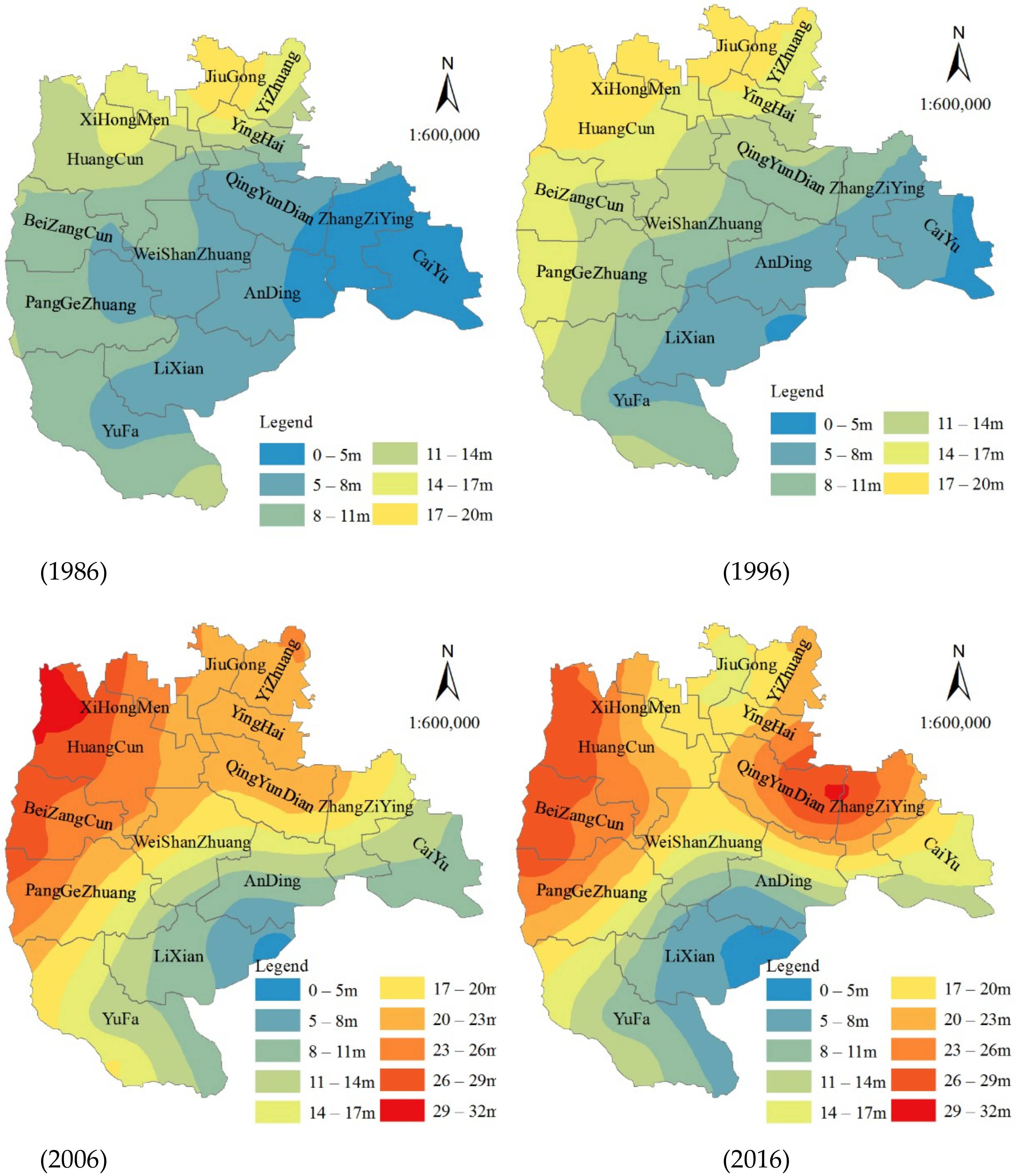
• The spatial interpolation of groundwater table depth in the study area from 1986 to 2016 is conducted using the OK method. The interpolation results showed that the overall groundwater table depth in the Daxing District increased from 1986 to 2016. The rate of groundwater decline was fastest from 1996 to 2006, with an annual decline rate of 0.65 m. The region with the largest decline rate of groundwater table depth in the Daxing District from 1986 to 2016 is the central area, followed by the northern and southern areas. Groundwater downwelling funnels occurred in Qingyundian and Beizangcun in the central region, which tended to continuously spread outward.
• The nugget effect from 1986 to 2016 was calculated using the geostatistical variation function model, which showed that the nugget effect of groundwater table depth increased continuously. The spatial correlation gradually weakened from 1986 to 2016. From 1986 to 2005, the effect of natural structural factors on the burial depth played a dominant role. From 2006 to 2016, human extraction activities have become important factors affecting the burial depth of the water table.
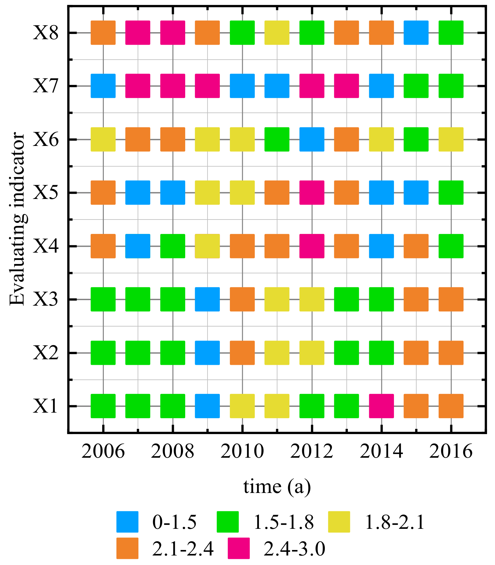
• The evaluation grade of groundwater exploitation intensity in the Daxing District from 2006 to 2016 was calculated using set pair analysis. The subtraction set pair potential was used to identify the key regulation years and the main factors affecting groundwater exploitation intensity. The results show that the groundwater extraction intensity in the Daxing area is moderate (grade II) with a bleak gradual deterioration trend. The evaluation results in 2010 and 2013, the years of key regulation of groundwater exploitation intensity, are partial negative potential and negative potential, respectively. The comprehensive evaluation results are 2.31 and 2.45, respectively. In 2010, three indicators had partial negative potential: industrial GDP, tertiary industry GDP, and irrigation area. In 2013, five indicators had negative potential: the irrigation area, vegetable area, facility agriculture area, fruit tree area, and number of wells.

To conclude, in the process of urbanization in the study area, the influence of human exploitation on the water table depth is increasing. Therefore, to reduce the impact of human exploitation on the groundwater resources, the regional water table depth monitoring system must be improved to understand the dynamic changes in the water table depth in time. Then, the regional total water consumption and the water consumption of each water-using sector must be analyzed and evaluated to understand the change in the groundwater exploitation intensity in that year and the main water-using sector that caused the change in the groundwater exploitation intensity. Based on the above analysis results of groundwater consumption and groundwater exploitation intensity, it provides the basis for groundwater exploitation planning and industrial regulation policy in the next year. Finally, unconventional water sources should be actively developed, and areas with water diversion conditions should actively strive for external water sources to reduce groundwater exploitation.

References

1. Zhang, A.J.; Ye, C. Beijing Groundwater, 1st ed.; Geological Publishing House: Beijing, China, 2008; pp. 122–126. [Google Scholar]
2. Zhang, Z.; Guo, H.; Zhao, W.; Liu, S.; Cao, Y.; Jia, Y. Influences of groundwater extraction on flow dynamics and arsenic levels in the western Hetao Basin, Inner Mongolia, China. Hydrogeol. J. 2018, 26, 1499–1512. [Google Scholar] [CrossRef]
3. Sahoo, S.; Russo, T.A.; Elliott, J.; Foster, I. Machine learning algorithms for modeling groundwater level changes in agricultural regions of the U.S. Water Resour. Res. 2017, 53, 3878–3895. [Google Scholar] [CrossRef]
4. Chen, M.; Tomás, R.; Li, Z.; Motagh, M.; Li, T.; Hu, L.; Gong, H.; Li, X.; Yu, J.; Gong, X. Imaging Land Subsidence Induced by Groundwater Extraction in Beijing (China) Using Satellite Radar Interferometry. Remote Sens. 2016, 8, 468. [Google Scholar] [CrossRef] [Green Version]
5. Pellicone, G.; Caloiero, T.; Modica, G.; Guagliardi, I. Application of several spatial interpolation techniques to monthly rainfall data in the Calabria region (southern Italy). Int. J. Climatol. 2018, 38, 3651–3666. [Google Scholar] [CrossRef]
6. Thiesen, S.; Vieira, D.M.; Mälicke, M.; Loritz, R.; Wellmann, J.F.; Ehret, U. Histogram via entropy reduction (HER): An information-theoretic alternative for geostatistics. Hydrol. Earth Syst. Sci. 2020, 24, 4523–4540. [Google Scholar] [CrossRef]
7. Ohmer, M.; Liesch, T.; Goeppert, N.; Goldscheider, N. On the optimal selection of interpolation methods for groundwater contouring: An example of propagation of uncertainty regarding inter-aquifer exchange. Adv. Water Resour. 2017, 109, 121–132. [Google Scholar] [CrossRef]
8. Adhikary, P.P.; Dash, C. Comparison of deterministic and stochastic methods to predict spatial variation of groundwater depth. Appl. Water Sci. 2017, 7, 339–348. [Google Scholar] [CrossRef] [Green Version]
9. Uc Castillo, J.L.; Ramos Leal, J.A.; Martínez Cruz, D.A.; Rodríguez Robles, U.; Cervantes Martínez, A.; Marín Celestino, A.E. Identification of the Dominant Factors in Groundwater Recharge Process, Using Multivariate Statistical Approaches in a Semi-Arid Region. Sustainability 2021, 13, 11543. [Google Scholar] [CrossRef]
10. Bronowicka-Mielniczuk, U.; Mielniczuk, J.; Obroślak, R.; Przystupa, W. A Comparison of Some Interpolation Techniques for Deter-mining Spatial Distribution of Nitrogen Compounds in Groundwater. Int. J. Environ. Res. 2019, 13, 679–687. [Google Scholar] [CrossRef] [Green Version]
11. Fazeli Sangani, M.; Namdar Khojasteh, D.; Owens, G. Dataset characteristics influence the performance of different inter-polation methods for soil salinity spatial mapping. Environ. Monit. Assess. 2019, 191, 1–12. [Google Scholar] [CrossRef]
12. Karami, S.; Madani, H.; Katibeh, H.; Marj, A. Assessment and modeling of the groundwater hydrogeochemical quality param-eters via geostatistical approaches. Appl. Water Sci. 2018, 8, 1–13. [Google Scholar] [CrossRef] [Green Version]
13. Zafor, M.A.; Alam, M.J.B.; Rahman, M.A.; Amin, M.N. The analysis of groundwater table variations in Sylhet region, Bangladesh. Environ. Eng. Res. 2017, 22, 369–376. [Google Scholar] [CrossRef] [Green Version]
14. Chandan, K.S.; Yashwant, B.K. Optimization of Groundwater Level Monitoring Network Using GIS-based Geostatistical Method and Multi-parameter Analysis: A Case Study in Wainganga Sub-basin, India. Chin. Geogr. Sci. 2017, 27, 201–215. [Google Scholar] [CrossRef] [Green Version]
15. Hussain, M.M.; Bari, S.H.; Tarif, M.E.; Rahman, M.T.U.; Hoque, M.A. Temporal and spatial variation of groundwater level in Mymensingh district, Bangladesh. Int. J. Hydrol. Sci. Technol. 2016, 6, 188. [Google Scholar] [CrossRef]
16. Zhang, H.; Wang, X.S. The impact of groundwater depth on the spatial variance of vegetation index in the Ordos Plateau, China: A semivariogram analysis. J. Hydrol. 2020, 588, 125096. [Google Scholar] [CrossRef]
17. Yin, S.; Gu, X.; Xiao, Y.; Wu, W.; Pan, X.; Shao, J.; Zhang, Q. Geostatistics-based spatial variation characteristics of groundwater levels in a wastewater irrigation area, northern China. Water Sci. Technol. Water Supply 2017, 17, 1479–1489. [Google Scholar] [CrossRef]
18. Wakode, H.B.; Baier, K.; Jha, R.; Azzam, R. Impact of urbanization on groundwater recharge and urban water balance for the city of Hyderabad, India. Int. Soil Water Conserv. Res. 2018, 6, 51–62. [Google Scholar] [CrossRef]
19. Yue, H.; Liu, Y. Water balance and influence mechanism analysis: A case study of Hongjiannao Lake, China. Environ. Mental. Monit. Assess. 2021, 193, 1–17. [Google Scholar] [CrossRef] [PubMed]
20. Mahmoudpour, M.; Khamehchiyan, M.; Nikudel, M.R.; Ghassemi, M.R. Numerical simulation and prediction of regional land subsid-ence caused by groundwater exploitation in the southwest plain of Tehran, Iran. Eng. Geol. 2016, 201, 6–28. [Google Scholar] [CrossRef]
21. Dash, C.; Sarangi, A.; Singh, D.K.; Adhikary, P.P. Numerical simulation to assess potential groundwater recharge and net ground-water use in a semi-arid region. Environ. Monit. Assess. 2019, 191, 1–14. [Google Scholar] [CrossRef]
22. Négrel, P.; Petelet-Giraud, E.; Widory, D. Strontium isotope geochemistry of alluvial groundwater: A tracer for ground-water resources characterisation. Hydrol. Earth Syst. Sci. 2004, 8, 959–972. [Google Scholar] [CrossRef]
23. Yue, C.F.; Wang, Q.J.; Li, Y.Z. Evaluating water resources allocation in arid areas of northwest China using a projection pursuit dynamic cluster model. Water Supply 2019, 19, 762–770. [Google Scholar] [CrossRef]
24. Tian, R.; Wu, J. Groundwater quality appraisal by improved set pair analysis with game theory weightage and health risk estimation of contaminants for Xuecha drinking water source in a loess area in Northwest China. Hum. Ecol. Risk Assess. Int. J. 2019, 25, 132–157. [Google Scholar] [CrossRef]
25. Giao, N.T.; Nhien, H.T.H.; Anh, P.K.; Van Ni, D. Classification of water quality in low-lying area in Vietnamese Mekong delta using set pair analysis method and Vietnamese water quality index. Environ. Monit. Assess. 2021, 193, 1–16. [Google Scholar] [CrossRef] [PubMed]
26. Jin, J.L.; Shen, S.X.; Li, J.Q.; Cui, Y.; Wu, C.G. Assessment and Diagnosis Analysis Method for Regional Water Resources Carrying Capac-ity Based on Connection Number. J. North China Univ. Water Resour. Electr. Power 2018, 39, 1–9. [Google Scholar] [CrossRef]
27. Yang, Y.F.; Wang, H.R.; Zhao, W.J.; Yan, G.W. Evaluation Model of Water Resources Carrying Capacity Based on Set Pair Potential and Partial Connection Number. Adv. Eng. Sci. 2021, 53, 99–105. [Google Scholar] [CrossRef]
28. Yang, H.M.; Zhao, K.Q. The calculation and application of partical connection numbers. CAAI Trans. Intell. Syst. 2019, 14, 865–876. [Google Scholar] [CrossRef]
29. Cambardella, C.A.; Moorman, T.B.; Novak, J.M.; Parkin, T.B.; Karlen, D.L.; Turco, R.F.; Konopka, A.E. Field-Scale Variability of Soil Properties in Central Iowa Soils. Soil Sci. Soc. Am. J. 1994, 58, 1501–1511. [Google Scholar] [CrossRef]
30. Gao, F.; Wang, H.X.; Liu, C.M. Variation in groundwater resources carrying capacity in Beijing between 2001 and 2015. Chin. J. Eco-Agric. 2019, 27, 1088–1096. [Google Scholar] [CrossRef]
31. Yu, H.Z.; Li, L.J.; Li, J.Y. Evaluation of water resources carrying capacity in the Beijing-Tianjin-Hebei Region based on quantity-quality-water bodies-flow. Resour. Sci. 2020, 42, 02000358. [Google Scholar] [CrossRef]
32. Li, Y.L.; Guo, X.N.; Guo, D.Y.; Wang, X.H. An evaluation method of water resources carrying capacity and application. Prog. Geogr. 2017, 36, 342–349. [Google Scholar] [CrossRef] [Green Version]
33. Jin, J.L.; He, P.; Zhang, H.Y.; Li, J.Q.; Chen, M.L.; He, J. Subtractive full neighbor connection number and its application in trend analysis of re-gional water resources carrying capacity. J. Northwest Univ. 2020, 50, 438–446. [Google Scholar] [CrossRef]
Figure 1. Geographic location map of the study area.
Sustainability 14 04341 g001
Figure 2. Variation of water table depth from 1986 to 2016.
Sustainability 14 04341 g002
Figure 3. Groundwater exploitation intensity in the Daxing District from 2006 to 2016.
Sustainability 14 04341 g003
Figure 4. Subtraction set potential of each evaluation index in the Daxing District from 2006 to 2016.
Sustainability 14 04341 g004
Figure 5. Evaluation grade of each evaluation index in the Daxing District from 2006 to 2016.
Sustainability 14 04341 g005