Forecasting the Volatility of European Union Allowance Futures with Climate Policy Uncertainty Using the EGARCH-MIDAS Model

Abstract

We propose the EGARCH-MIDAS-CPU model, which incorporates the leverage effect and climate policy uncertainty (CPU) to model and forecast European Union allowance futures’ (EUAF) volatility. An empirical analysis based on the daily data of the EUAF price index and the monthly data of the CPU index using the EGARCH-MIDAS-CPU model shows that the EUAF’s volatility exhibits a leverage effect, and the CPU has a significantly negative impact on the EUAF’s volatility. Furthermore, out-of-sample analysis based on three loss functions and the Model Confidence Set (MCS) test suggests that EGARCH-MIDAS-CPU model yields more accurate out-of-sample volatility forecasting results than various competing models. There is room for further application of the model, such as this model could be applied to price carbon futures, so as to improve the liquidity of the carbon market and achieve carbon peak and carbon neutrality as soon as possible.

1. Introduction

With the continuous development of industry and science and technology, people’s living environment has been deteriorating. In order to improve people’s living environment and ensure the sustainable development, the European Union established the Emission Trading System (EU ETS), which was set up to mitigate the environmental press about carbon emissions. European Union allowance futures (EUAF) have been sold in the market since the EU ETS was established, and the EUAF have played a crucial role in derivative products. Modeling and forecasting the EUAF’s volatility could effectively capture EUAF market risk and optimize the market risk management mechanism.

Carbon is a natural product, which is inevitably affected by climate change. The EUAF are carbon financial derivative products, and they are also inevitably affected by climate change and economic policy changes. The existing literature demonstrates that climate change and policy uncertainty adjustment would affect carbon futures’ price fluctuation [1], the impact of climate change and policy adjustment uncertainty on carbon futures price is analyzed from the following three perspectives. First, based on demand perspective, residents would increase the demand for carbon products when the sudden climate change occurs. Increasing consumption demand of carbon products would promote enterprises to increase production, and enterprises would purchase the carbon emissions products when the carbon emissions reach the upper limitations, which could reduce carbon emissions and accelerate carbon market development [2]. Then, based on the supply perspective, when extreme climate change occurs, the crude material not being supplied in time leads to an increase in the cost of carbon emissions. To reduce the cost of purchasing the crude material of carbon, enterprises would mitigate carbon emissions. Lastly, based on the social welfare perspective, the demand and supply would create an imbalance when climate change occurs, and the government would sustain the balance of carbon price for society [3].

It could be concluded from the above analysis that climate change would impact the carbon price fluctuation, but climate change has been difficult to accurately forecast. Meanwhile, climate change generates economic policy uncertainty adjustments that cannot be forecast. Hence, there are fewer scholars researching the relationship between climate policy uncertainty and EUAF volatility. There are two reasons to explain this phenomenon: One is that it is uneasy to measure the climate policy uncertainty; the other is that there is not a suitable model to demonstrate the relationship between themselves.

Gavriilidis [4], based on major American newspapers and the latest laws about carbon emissions, such as the global strike on climate change and the president’s statement on climate policy, constructed the climate policy uncertainty (CPU) index. We use the CPU to research the relationship between the CPU and EUAF volatility and to explore whether the model containing the CPU yields more accurate out-of-sample volatility forecasting results. CPU is a monthly index, and the EUAF price is a daily index. The data frequency of the two indicators is inconsistent. If the daily data of EUAF price is converted into monthly data, important information contained in the daily data will be lost, leading to deviation in the empirical results. Therefore, it is important to select a suitable model that could contain different frequencies of data to research the relationship between CPU and EUAF volatility and to explore the prediction ability of CPU to EUAF volatility.

In the view of this, Engle et al. [5] combined the GARCH model with the mixed frequency data sampling (MIDAS) model to propose the GARCH-MIDAS model, the significant characteristic of the GARCH-MIDAS model is that volatility is divided into the short-term and long-term components. The short-term component was modeled by daily return, and the long-term component was modeled by low-frequency (monthly) variables. The GARCH-MIDAS model could not only capture the influence from different frequencies of data to volatility, but the volatility forecasting ability of GARCH-MIDAS model outperform the traditional GARCH-type models. Therefore, the GARCH-MIDAS model has focused on the stock market [6,7,8], the futures market [9], foreign exchange market [10,11] and energy market [12,13,14].

However, GARCH-MIDAS model has a drawback, which could not capture the leverage effect of volatility. Hence, we propose the EGARCH-MIDAS-CPU model that contained the CPU. Comparing the EGARCH-MIDAS-CPU model with the GARCH-MIDAS model, this model could not only capture the leverage effect of volatility but could also explore the relationship between CPU and EUAF volatility and study whether the introduction of CPU could improve the prediction accuracy of EUAF volatility.

The innovations of the paper are twofold. First, we propose the EGARCH-MIDAS-CPU model framework combing the CPU index. Compared to benchmark models (GARCH, GARCH-MIDAS, GARCH-MIDAS-CPU model), the EGARCH-MIDAS model allows us to capture the leverage effect of EUAF volatility. Second, we study the relationship between CPU and EUAF volatility, and find that the CPU has a significantly negative impact on the EUAF’s volatility. Moreover, CPU could improve the forecast accuracy for the EUAF’s volatility. Most importantly, we find that the superior forecast ability of EGARCH-MIDAS-CPU model is robust to short-term and medium-term forecasting windows.

The remainder of this paper is organized as follows. Section 2 presents the literature review. Section 3 introduces methodology and data. Section 4 reports the results. Section 5 provides the further discussion. Section 6 makes a conclusion.

2. Literature Review

As one of the most important characteristics of carbon futures, the modeling and prediction of carbon futures volatility can not only measure the risk in the carbon futures market but can also provide reference for investors to formulate hedging strategies and policy makers to formulate corresponding risk management regulations. Therefore, it is of great theoretical and practical significance to accurately model and forecast the carbon futures’ volatility. The volatility prediction model has employed the generalized autoregressive conditional heteroscedasticity (GARCH) model [15]. The hypothesis of volatility in the GARCH model is the certainty function about historical information, and parameters are easily estimated by the maximum likelihood function. Therefore, the GARCH model has been employed to model and forecast volatility in many areas.

However, the GARCH model has many defects in modeling volatility. On the one hand, the GARCH model could not capture the asymmetry of volatility. Conrad et al. [16] used the asymmetric GARCH-type models to capture the dynamic characteristics of the EUAF’s volatility, and demonstrated that the EUAF’s volatility exists as asymmetric characteristic (leverage effect). Dutta et al. [17] explored the relationship of EUAF and the implied volatility of crude oil by using the EGARCH model, which contains a dynamic jump component. The result of empirical research found that not only is there a high correlation between two markets, but the volatility of both markets has a leveraging effect. Zhang et al. [18] conducted an empirical study for China’s carbon emission markets’ volatility by using the EGARCH model and found that China’s carbon emission markets have “the counter leverage effect”, which means that China’s carbon emission markets have severe reaction to good news rather than bad news after policies were published.

On the other hand, GARCH-type models (GARCH and EGARCH model) also could not consider the existence of exogenous variables that could affect the EUAF’s volatility. For example, energy markets (coal, carbon, crude oil, and nature gas, etc.) affect the carbon emissions markets’ volatility [19,20], as well as the economy and policy [21,22]. In addition, Wang et al. [13] found the relationship of the EUAF and climate change and uncovered the close connection between the EUAF’s volatility and climate change. Batten et al. [23] explored the connection of energy markets, extreme change in climate, and EUAF and demonstrated that extreme change in climate would affect the volatility of EUAF. Gugler et al. [24] demonstrated the effectiveness of England and Germany in reducing carbon emissions from the perspective of climate policy. Hambel et al. [25] constructed the equilibrium model about climate change and systematically analyzed the relationship between climate uncertainty and the social cost of carbon emissions.

Climate change and policy adjustments have a significant uncertainty. There are many papers measuring the climate policy uncertainty. The climate policy uncertainty (CPU) has been used in many areas since the CPU index was proposed. Lopez et al. [26] found a positive correlation between uncertainty caused by climate policies and reduced corporate investment from a sample of 250 European companies. Golub et al. [27] illustrated that earning profit is not stable in risk-neutral conditions, and the CPU would be a hinderance for enterprises to make investments and take loans from banks in reducing carbon emissions. Based on the above analysis, we could find that the study of the CPU concentrates on investors, enterprises, and banks. Fewer scholars have studied the relationship between the CPU and the carbon futures market, and the CPU maybe have some abilities to explain and predict EUAF price fluctuation. Therefore, we use the CPU to research the relationship between it and the EUAF’s volatility and, at the same time, to see whether the introduction of the CPU index into models could improve the EUAF volatility prediction accuracy.

In the past, the GARCH model was used to forecast the volatility of carbon financial products. For example, Huang et al. [28] used the GARCH model to research and forecast the EUAF’s volatility and found that the single-factor GARCH model did not yield the accuracy in volatility forecasting, but extended GARCH models could yield higher prediction accuracy in predicting EUAF volatility. Zhao et al. [29] researched the relationship between energy markets and the EUAF’s volatility by using the mixed frequency data sampling (MIDAS) model and found that the MIDAS model could capture the effective information in mixed energy and economic variables and that the model containing a MIDAS component could predict the EUAF’s volatility very well. In view of this, Dai et al. [30] used the GARCH-MIDAS model to research the impact of economic policy uncertainty on EUA spot volatility and found that economic policy uncertainty would affect the long-term volatility of the EUA’s spot volatility. Meanwhile, the model containing economic uncertainty would improve the EUA’s spot volatility forecasting accuracy. Liu et al. [31] researched the relationship between economic policy uncertainty and the EUAF’s volatility by using the GARCH-MIDAS model and demonstrated that economic policy uncertainty would affect the EUAF’s volatility and that the GARCH-MIDAS model containing economic policy uncertainty outperformed the GARCH-type models in EUAF volatility prediction.

In this paper, we propose the EGARCH-MIDAS-CPU model to model and forecast volatility. The outstanding advantage of this model is that it could not only obtain the superior forecasting ability of GARCH-MIDAS model, but also could capture the leverage effect of EUAF volatility. Therefore, it is reasonable to use the EGARCH-MIDAS-CPU model to analyze and predict EUAF volatility. The empirical results also show that the out-of-sample prediction accuracy of EGARCH-MIDAS-CPU model outperforms that of GARCH-type models, which provides a new perspective for modeling and predicting EUAF volatility.

3. Methodology and Data

3.1. EGARCH-MIDAS-CPU Model

We propose an EGARCH-MIDAS-CPU model that could combine data of different frequencies. The expression of the model is as follows:

$$r_{i,t}=\mu +{\sigma }_{i,t}{ϵ}_{i,t},\forall i=1,\dots ,N_t$$

(1)

$${\sigma }_{i,t}^2=g_{i,t}{\tau }_t$$

(2)

$${ϵ}_{i,t}|{\mathrm{\Phi }}_{i-1,t}~i.i.d.N(0,1)$$

(3)

where $r_{i,t}$ denotes the logarithmic return day $i$ of month $t$, namely, $r_{i,t}=log{P}_{i,t}-log{P}_{i-1,t}$, and $P_{i,t}$ is the price of futures day $i$ of $t$ month. ${ϵ}_{i,t}$ is independent identically distributed standard normally distributed random variables at the set of ${\mathrm{\Phi }}_{i-1,t}$.

It can be seen in Equation (2) that the conditional variance of the daily return is divided into two components: a short-term $g_{i,t}$ and a long-term ${\tau }_t$. The short-term $g_{i,t}$ follows the EGARCH (1,1) process:

$$log(g_{i,t})=\gamma {ϵ}_{i-1,t}+\alpha (\left|{ϵ}_{i-1,t}\right|-E(\left|{ϵ}_{i-1,t}\right|)+\beta log(g_{i-1,t}))$$

(4)

where $\beta <1$ sustains the sequence stable, $\gamma$ is a coefficient of leverage effect, if $\gamma <0$ shows that negative impact on the EUAF volatility is greater than that of positive impact on the EUAF volatility under the same conditions, and vice versa.

The form of the long-term component, the regression formula of MIDAS model, is used in this paper that was derived from Dai et al. [32] and Liu et al. [8]; the expression of ${\tau }_t$ is as follows:

$$log({\tau }_t)=m+{\theta }_1{\displaystyle \sum _{k=1}^K{\psi }_k}({\omega }_1)log(R{V}_{t-k})+{\theta }_2{\displaystyle \sum _{k=1}^K{\psi }_k}({\omega }_2)log(CP{U}_{t-k})$$

(5)

where $m$ is an intercept term, ${\theta }_1$ is the influence coefficient of $RV$ on long-term component ${\tau }_t$, ${\theta }_2$ is the influence coefficient of the CPU on the long-term component. If ${\theta }_2>0$, this indicates that there is a positive correlation between climate policy uncertainty and long-term EUAF volatility. If ${\theta }_2<0$, this indicates that there is a negative correlation between climate policy uncertainty and long-term EUAF volatility, namely, improving the value of the CPU would mitigate the long-term EUAF volatility in the future. $K$ is the maximum MIDAS lag order of the low-frequency variables. ${\psi }_k(\omega )$ is the Beta weight function. Consistent with Yu et al. [33], we set the Beta weight function as follows:

$${\psi }_k(\omega )=\frac{{(1-k/K)}^{\omega -1}}{{\displaystyle \sum _{j=1}^K{(1-k/K)}^{\omega -1}}}$$

(6)

$R{V}_t$ is the monthly volatility, based on the square sum of the daily rates of return:

$$R{V}_t={\displaystyle \sum _{i=1}^{N_t}{r}_{i,t}^2}$$

(7)

where $N_t$ is the total number of trading days in the $t$ month. The EGARCH-MIDAS-CPU model is constructed by Equations (1)–(7), namely, considering the leverage effect and CPU that could affect the EUAF volatility.

3.2. Model Maximum Likelihood Estimation

The parameters of the EGARCH-MIDAS-CPU model could be estimated by using the maximum likelihood function. The logarithmic likelihood function of the model is derived as follows:

$$\mathcal{\ell }(r;\mathrm{\Theta })=-\frac{1}{2}{\displaystyle \sum _{t=1}^T{\displaystyle \sum _{i=1}^{N_t}[}}\log (2\pi )+\log (g_{i,t}{\tau }_t)+\frac{{(r_{i-1,t}-\mu )}^2}{\log (g_{i,t}{\tau }_t)}]$$

(8)

where $N_t$ and $t$ denote the total number of trading days in the month of $t$ and the total number of months in transaction data, respectively.$\mathrm{\Theta }=(\mu ,m,{\theta }_1,{\theta }_2,{\omega }_1,{\omega }_2,\gamma ,\alpha ,\beta {)}^{\prime }$ is the vector set of parameters. Furthermore, the maximum likelihood estimate of model parameters can be obtained by maximizing the logarithmic likelihood function:

$$\widehat{\mathrm{\Theta }}=\underset{\mathrm{\Theta }}{arg\max \mathcal{\ell }(R;\mathrm{\Theta })}$$

(9)

3.3. Model Maximum Likelihood Estimation

We choose the GARCH, GARCH-MIDAS, and GARCH-MIDAS-CPU models as the benchmark models to demonstrate the superiority of data fitting and prediction ability of the EGARCH-MIDAS-CPU model. In order to make the models comparable, we set the GARCH model to follow the GARCH (1,1) process, and the presentation of the GARCH model is as follows:

$$r_t=\mu +{\sigma }_t{ϵ}_t$$

(10)

$${\sigma }_t^2=m+\alpha {({\sigma }_{t-1}{ϵ}_{t-1})}^2+\beta {\sigma }_{t-1}^2$$

(11)

$${ϵ}_t|{\mathrm{\Phi }}_{t-1}~i.i.d.N(0,1)$$

(12)

where $r_t$ denotes to the logarithmic return on day of t, namely, $r_t=log{P}_t-log{P}_{t-1}$. $\mu$ is conditional mean of $r_t$, where $\alpha$, $\beta$ are the parameters of ARCH and GARCH components, respectively, where $0<\alpha$ and $0<\beta$, and $\alpha +\beta <1$. The GARCH model is constructed by Equations (10)–(12).

The GARCH-MIDAS model and the GARCH-MIDAS-CPU model have the same short-term components. In order to make a comparison, we set the short-term volatility components in accordance with the GARCH (1,1) process:

$$r_{i,t}=\mu +{\sigma }_{i,t}{ϵ}_{i,t},\forall i=1,\dots ,N_t$$

(13)

$${\sigma }_{i,t}^2=g_{i,t}{\tau }_t$$

(14)

$$g_{i,t}=(1-\alpha -\beta )+\alpha \frac{{(r_{i-1,t}-\mu )}^2}{{\tau }_t}+\beta g_{i-1,t}$$

(15)

The long-term component of GARCH-MIDAS model is as follows:

$$log({\tau }_t)=m+{\theta }_1{\displaystyle \sum _{k=1}^K{\psi }_k}({\omega }_1)log(R{V}_{t-k})$$

(16)

The setting form of the long-term component of the GARCH-MIDAS-CPU model is the same as the form of Equation (5), which is not repeated here.

3.4. Data and Statistical Description

Since the EU ETS was established, the EU ETS has finished three phases and has been working on its fourth phase: phase I: from 3 January 2005 to 31 December 2007; phase II: from 2 January 2008 to 31 December 2012; phase III: from 2 January 2013 to 31 December 2020; and phase IV: from 4 January 2021 to 31 December 2030. Because phase I is a trial stage, the EU ETS was restricted in bank loans at the end of phase I that resulted in the price of the EUAF tending to be zero [33]. This paper chose phase II to phase IV to conduct empirical research; the data period is contained from 2 January 2008 to 31 March 2021, with 3410 data from the WIND database. The CPU is derived from http://www.policyuncertainty.com/ (accessed on 25 April 2021) website, that is, constructed by Gavriilidis [5]. The sample is selected from January 2008 to March 2021, with 159 monthly data.

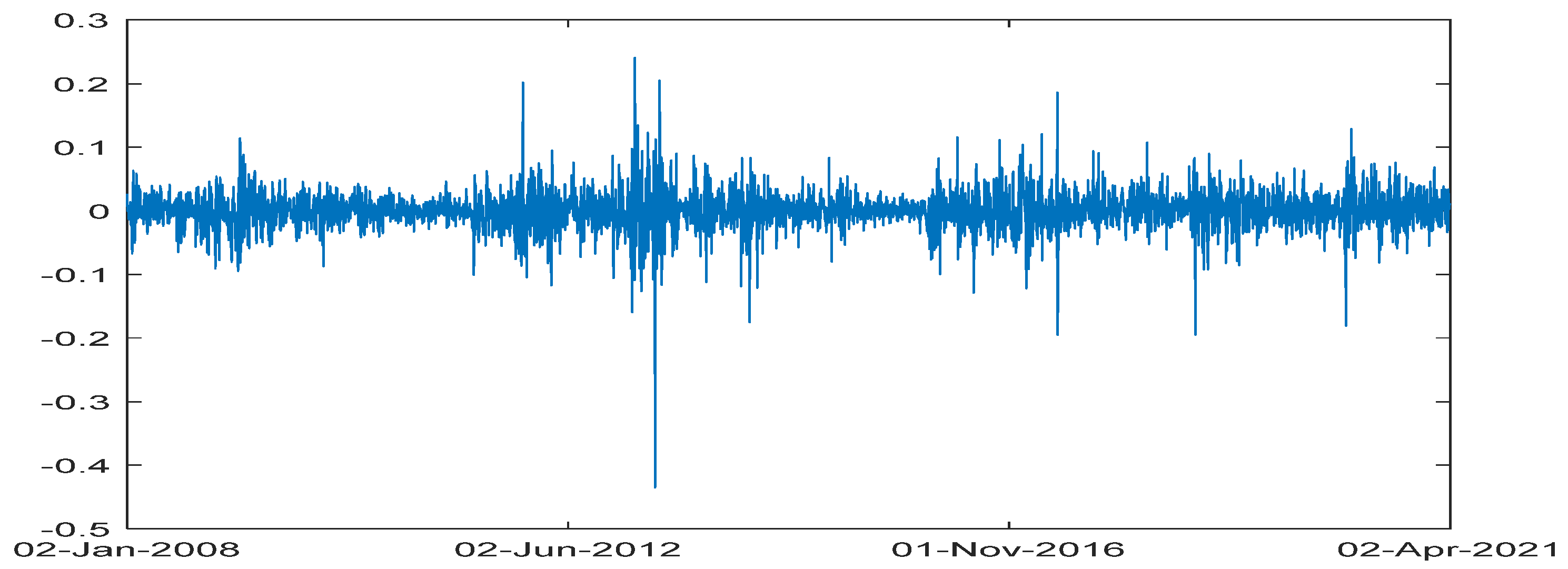
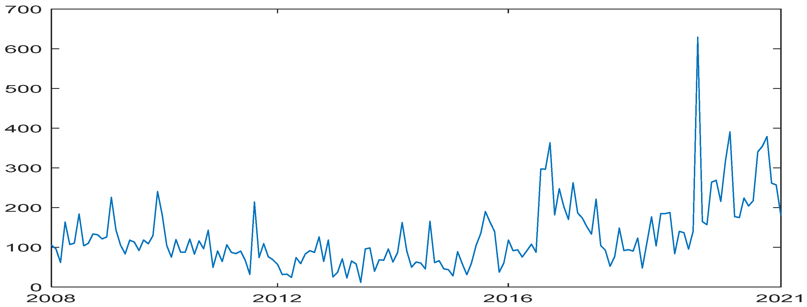
Figure 1 displays the time series of the EUAF returns, the returns of EUAF presents clustering. We found that Figure 2 climate change shows obvious difference from the time series of CPU. Especially after the Paris Agreement was signed and the outbreak of COVID-19, the CPU change has been bigger than before. In addition, we could obtain a result from the comparison between the EUAF return and CPU figure that when the CPU fluctuates greatly, the return would significantly change.

Table 1. Statistical description.

	Obs	Mean	Min	Max	Std	Skewness	Kurtosis	J-B	Q(10)
r	3409	0.0002	−0.4347	0.2405	0.0315	−0.7665	18.3156	33652.0038	32.5790
CPU	159	128.1951	11.7800	629.0200	86.0910	2.0870	10.068	446.3868	265.4308

Note: J-B represents Jarque–Bera statistic, and Q (10) represents LJung-Box Q statistic with a lag of 10 orders.

shows the descriptive statistics of EUAF’s return and the CPU index. The skewness is less than 0, and the kurtosis is bigger than 3, which deviates significantly from the normal distribution. Comparison of the value of $r$ and the CPU found that the CPU has the bigger mean and standard deviation; this indicates that the CPU index has a large fluctuation.

4. Results

4.1. Estimation Results

We choose the GARCH, GARCH-MIDAS, GARCH-MIDAS-CPU, and EGARCH-MIDAS-CPU models to conduct empirical research for the sample period from 2 January 2008 to 31 December 2018, with 2830 data. The biggest lags order (K) of MIDAS of the GARCH-MIDAS, GARCH-MIDAS-CPU, and EGARCH-MIDAS-CPU models are set to 12, namely, employing the total information of the CPU filter of the last year obtains the long-term fluctuation of the EUAF. The parameter estimation results of the models are presented in

Table 2. Estimation results.

	GARCH	GARCH-MIDAS	GARCH-MIDAS-CPU	EGARCH-MIDAS-CPU
$\mu$	0.0010	0.0010	0.0010	0.0007
	(0.0004)	(0.0004)	(0.0004)	(0.0006)
$m$	0.0000	−3.9721	−3.5619	−3.0748
	(0.0000)	(0.1189)	(0.1048)	(0.1204)
${\theta }_1$		0.6319	0.6446	0.5869
		(0.0248)	(0.0188)	(0.0349)
${\theta }_2$			−0.0825	−0.3157
			(0.0197)	(0.0235)
${\omega }_1$		1.0043	0.9973	4.0518
		(0.0175)	(0.0189)	(0.1788)
${\omega }_2$			0.1158	0.9218
			(0.0000)	(0.0179)
$\gamma$				−0.0557
				(0.0158)
$\alpha$	0.1426	0.1541	0.1540	0.3026
	(0.0088)	(0.0089)	(0.0080)	(0.0205)
$\beta$	0.8544	0.8222	0.8213	0.9252
	(0.0087)	(0.0104)	(0.0102)	(0.0091)
$\mathcal{\ell }\left(r;\mathrm{\Theta }\right)$	6246.4271	6254.5821	6255.0531	6255.1814
AIC	−12,484.8542	−12,497.1642	−12,494.1062	−12,492.3627
BIC	−12,461.0621	−12,461.4760	−12,446.5219	−12,438.8304

Note: AIC and BIC denote the Akaike information criterion and Bayesian information criterion, respectively. The number in parenthesis is the standard error.

.

As can be seen from Table 2, the volatility persistence coefficient $\alpha +\beta$ of the GARCH-type models (GARCH, GARCH-MIDAS, and GARCH-MIDAS-CPU models) close to 1, and the volatility persistence coefficient of EGARCH-MIDAS-CPU is also close to 1, it demonstrates that the short-term EUAF’s volatility has the highest level of volatility persistence. The parameter estimation result of $\gamma$ shows that the EUAF volatility exhibits a leverage effect. That is, the negative impact on the EUAF volatility is greater than the positive impact on the EUAF volatility under the same conditions.

Then, the parameter estimation results of ${\omega }_1$ and ${\theta }_1$ are significant, namely, RV has a positive effect in the long-term EUAF volatility. That is, the bigger fluctuation in the RV would cause the bigger long-term EUAF fluctuation. In addition, ${\omega }_2$ and ${\theta }_2$ are significant, that means that the lag information of the CPU could not only affect the long-term fluctuation in the EUAF, but the impact is also significantly negative [14]; that is, the higher value of the CPU could forecast the lower long-term EUAF volatility. The explanation is that when drastic climate change, the EUAF volatility would wildly fluctuate, government would publish some regulations to mitigate the EUAF volatility for achieving carbon peak and carbon neutral targets, some policies would be published for price stabilization, the relationship between these are negative, so the relationship of the CPU and EUAF volatility is negative.

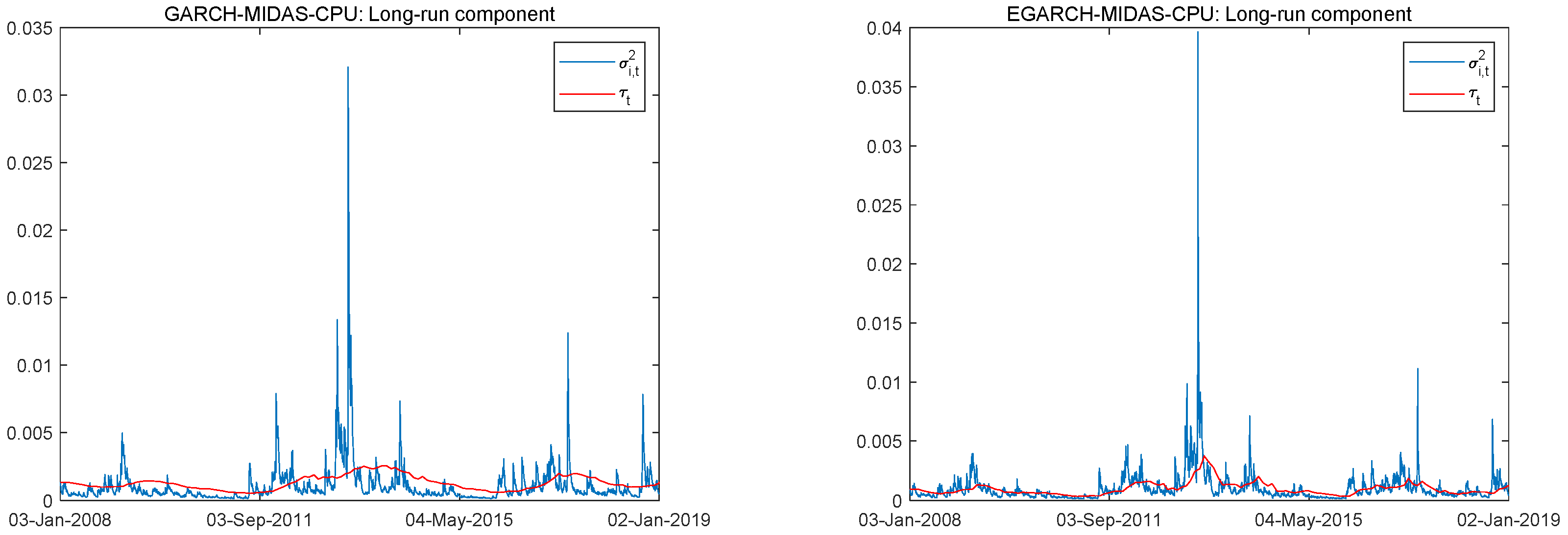
As can be seen from Figure 3, the long-term component fitting effect of EGRCH-MIDAS-CPU model is significantly better than that of the GARCH-MIDAS-CPU model. It further shows that the EGARCH-MIDAS-CPU model can better fit the data of the EUAF market, considering the asymmetry of the volatility of EUAF and the influence of CPU on the volatility of the EUAF market.

4.2. Out-of-Sample Results

Investors would be more interested in out-of-sample predictive ability of the models and the indicators that could accurately predict future volatility than the estimated results in a sample. We employ a rolling time window scheme to prove the predictive ability of the EGARCH-MIDAS-CPU model. The timespan from 2 January 2019 to 31 March 2021 obtains the 579 out-of-sample predictive samples. In this paper, three loss functions would be used to evaluate the prediction performance of the models. Mean Absolute Error (MAE), Mean Squared Error (MSE), and Quasi-likelihood (QLIKE) are shown in Equations (17)–(19), respectively:

$$MAE=\frac{1}{T}{\displaystyle \sum _{t=1}^T|{\sigma }_{t+1}^2-{\widehat{\sigma }}_{t+1}^2(m)|}$$

(17)

$$MSE=\frac{1}{T}{\displaystyle \sum _{t=1}^T({\sigma }_{t+1}^2-{\widehat{\sigma }}_{t+1}^2(m))}$$

(18)

$$QLIKE=\frac{1}{T}{\displaystyle \sum _{t=1}^T(}\frac{{\sigma }_{t+1}^2}{{\widehat{\sigma }}_{t+1}^2(m)}-log(\frac{{\sigma }_{t+1}^2}{{\widehat{\sigma }}_{t+1}^2(m)})-1)$$

(19)

where $T$ is the numbers of out-of-sample forecasting, ${\sigma }^2$ represents the variance of the return rate of the EUAF. ${\widehat{\sigma }}^2(m)$ denotes the forecasting volatility proxy, and $m$ presents the GARCH, GARCH-MIDAS, GARCH-MIDAS-CPU, and EGARCH-MIDAS-CPU forecasting models.

As can be seen from the

Table 3. Out-of-sample results.

	GARCH	GARCH-MIDAS	GARCH-MIDAS-CPU	EGARCH-MIDAS-CPU
MAE	9.3879 × 10−4	9.3361 × 10−4	9.2028 × 10−4	8.9909 × 10−4
MSE	3.7593 × 10−6	3.7307 × 10−6	3.6968 × 10−6	3.6017 × 10−6
QLIKE	1.4042	1.4024	1.3939	1.4016

Note: The lowest ratio in each row is shown in bold.

, the EGARCH-MIDAS-CPU model could yield more accurate out-of-sample volatility forecasting results than the benchmark models (GARCH, GARCH-MIDAS, and GARCH-MIDAS-CPU models) in most cases. This illustrates that the model contained a leveraging effect, and the CPU could improve prediction accuracy for EUAF volatility forecasting. In addition, compared to the GARCH-type models (GARCH, GARCH-MIDAS, and GARCH-MIDAS-CPU models), we found that the GARCH-MIDAS-CPU model obtains a higher out-of-sample prediction accuracy on the whole, followed by the GARCH-MIDAS model and the GARCH model, which further prove that the models containing the CPU index could improve the volatility prediction accuracy of the models.

4.3. MCS Test Results

In order to test and evaluate out-of-sample prediction, the statistical significance of the EGARCH-MIDAS-CPU and benchmark models were assessed. The Model Confidence Set (MCS), proposed by Hansen et al. [34], is employed to identify optimal models with the certain reliability. Setting the $M^0$ is the original set of competition models, the null hypothesis is that the predictive ability of any two models is the same. The theorem-type environments (including propositions, lemmas, corollaries etc.) can be formatted as follows:

$$H_{0,M}:E(d_{uv,t})=0,\forall u,v\subset M^0,M^0\subset M$$

(20)

where $d_{uv}=Los{s}_t(u)-Los{s}_t(v)$ represents the difference between the loss function values of model u and v at the same loss function MAE, MSE, and QLIKE.

Based on equivalence test and elimination rules, the optimal prediction combination is selected to construct statistical test:

$$T_M=\underset{u,v\in \mathcal{M}}{Max}\left|t_{uv}\right|$$

(21)

where ${\overline{d}}_{uv}$ is the average difference in between any two prediction models ($u$ and $v$) relative to the loss function. $\widehat{Var}({\overline{d}}_{uv})$ represents the value of $Var({\overline{d}}_{uv})$ estimated using bootstrap method. When the statistical value of T is greater than the critical value, the null hypothesis is rejected and the poor prediction model is eliminated. The above process is repeated until there are no further models to be eliminated. Finally, the optimal prediction combination is obtained. For implementing the MCS procedure, we use a block bootstrap of ${10}^5$ replications and a significance level of 10%. According to the basic principle of MCS test, if the p-value of MCS test is less than 0.1, the model cannot pass the MCS test, which also indicates that the model has a poor volatility predictive ability. On the contrary, the model has a p value greater than 0.1, which could pass the MCS test, and it is a model with better volatility predictive ability.

As can be seen from

Table 4. MCS test results.

	GARCH	GARCH-MIDAS	GARCH-MIDAS-CPU	EGARCH-MIDAS-CPU
MAE	0.0042	0.0000	0.0478	1.0000
MSE	0.0579	0.1318	0.1318	1.0000
QLIKE	0.0791	0.0825	1.0000	0.3763

Note: The numbers in the table are the p-values of MCS test. p-values are greater than 0.1 (bold) indicate that the models are included in the MCS test, that is, the model with good volatility predictive ability.

, the EGARCH-MIDAS-CPU model not only passes the whole MCS test in three loss functions but also yields the biggest p value (p=1) in the most cases. Thus, the model containing the leverage effect and CPU could forecast the EUAF’s volatility very well. Meanwhile, the out-of-sample forecasting results of GARCH-type models are compared, the GARCH-MIDAS-type models (GARCH-MIDAS and GARCH-MIDAS-CPU models) outperform the GARCH model in the out-of-sample prediction. Furthermore, the GARCH-MIDAS-CPU model outperforms the GARCH-MIDAS model in most cases, and it could also demonstrate that the model contained CPU could improve volatility prediction accuracy.

5. Further Discussion

In order to test whether the out-of-sample forecasting abilities of the models are robust, this paper chooses different rolling time windows to perform out-of-sample forecasting. The out-of-sample forecasting periods are from 10 November 2020 to 31 March 2021, 23 June 2020 to 31 March 2021, and 25 April 2019 to 31 March 2021. The forecast intervals are 100, 200, and 500 days, respectively, to test whether the model constructed in this paper has robustness and applicability in different prediction periods.

Table 5. Out-of-sample results.

	GARCH	GARCH-MIDAS	GARCH-MIDAS-CPU	EGARCH-MIDAS-CPU
100
MAE	1.0696 × 10−3	1.0507 × 10−3	1.0410 × 10−3	9.9992 × 10−4
MSE	5.7411 × 10−6	5.6838 × 10−6	5.6475 × 10−6	5.5139 × 10−6
QLIKE	1.4459	1.4380	1.4308	1.4452
200
MAE	1.0036 × 10−3	9.8285 × 10−3	9.6551 × 10−3	9.3439 × 10−3
MSE	5.0822 × 10−6	5.0254 × 10−6	5.0053 × 10−6	4.8673 × 10−6
QLIKE	1.4533	1.4459	1.4467	1.4505
500
MAE	1.0612 × 10−3	1.0445 × 10−3	1.0376 × 10−3	9.862410−4
MSE	6.5978 × 10−6	6.5525 × 10−6	6.5554 × 10−6	6.4527 × 10−6
QLIKE	1.5346	1.5227	1.5307	1.5450

Note: The lowest ratio in each row is shown in bold.

and

Table 6. Out-of-sample results.

	GARCH	GARCH-MIDAS	GARCH-MIDAS-CPU	EGARCH-MIDAS-CPU
100
MAE	0.0003	0.0016	0.0024	1.0000
MSE	0.0483	0.0666	0.1198	1.0000
QLIKE	0.2109	0.2109	1.0000	0.2109
200
MAE	0.0000	0.0015	0.0132	1.0000
MSE	0.0569	0.1506	0.1506	1.0000
QLIKE	0.4582	1.0000	0.9172	0.9172
500
MAE	0.0000	0.0000	0.0000	1.0000
MSE	0.3132	0.6752	0.6752	1.0000
QLIKE	0.1185	1.0000	0.1644	0.1185

Note: The numbers in the table are the p-values of MCS test. p-values are greater than 0.1 (bold) indicate that the models are included in the MCS test, that is, the model with good volatility predictive ability.

show the different loss function values and MCS test results under different rolling time windows.

As can be seen from Table 5 and Table 6. In the short-term and medium-term, the model containing the CPU could improve the accuracy of volatility prediction. Furthermore, the EGARCH-MIDAS-CPU model could yield the highest out-of-sample prediction accuracy in the short-term and the medium-term, indicating that the model contained a leverage effect and the CPU could forecast EUAF volatility very well. However, in the long-term, the EGARCH-MIDAS-CPU model also obtains the highest accuracy in the most cases, but the prediction accuracy is not significantly compared to benchmark models.

6. Conclusions

EUAF volatility modeling and forecasting is of great significance for allocation assessment, hedging, and risk management. Therefore, it is significant to accurately forecast EUAF volatility, and it is also a hot research orientation in finance and energy. The traditional model does not take into account the leverage effect (asymmetry) of the EUAF’s volatility and the impact of climate policy uncertainty (CPU) on the EUAF’s volatility. To address this issue, this paper proposes an extension of the GARCH-MIDAS model, namely, the EGARCH-MIDAS-CPU model, which incorporates the leverage effect and CPU to model and forecast the EUAF’s volatility. An empirical analysis based on the daily data of the EUAF index and the monthly data of the CPU index shows that the EUAF’s volatility exhibits a leverage effect and the CPU has a significantly negative impact on the long-term component of the EUAF’s volatility. Furthermore, out-of-sample analysis based on three loss functions and the model confidence set (MCS) test suggests that EGARCH-MIDAS-CPU yields more accurate out-of-sample volatility forecasts than the benchmark models. In particular, the superior forecasting ability of the EGARCH-MIDAS-CPU model is robust to short-term and medium-term forecasting windows, but the robustness of the EGARCH-MIDAS-CPU model is not significant in the long-term forecasting window. Hence, the model, which contained the leverage effect and the CPU, could only yield more accurate out-of-sample volatility forecasts in the short and medium terms.

According to the conclusion of this paper, we discuss the economic value of this paper from the theoretical and practical aspects. From the theoretical point of view, the EGARCH-MIDAS-CPU model proposed in this paper not only fills in the blanks of EUAF volatility prediction but also clarifies the relationship between climate policy uncertainty and EUAF volatility, that is, how the change in climate policy would adversely affect the EUAF’s volatility. From a practical point of view, researching the relationship between CPU and EUAF volatility can help carbon emission enterprises analyze the relationship between climate policy changes and their own emission reduction costs, so as to adjust their emission strategies and achieve the purpose of energy conservation and emission reduction. It is helpful for policy makers to make reasonable risk avoidance policies based on climate policies and EUAF market fluctuations, promote the healthy and stable development of EUA market, and achieve the goal of carbon neutrality and carbon peak at an early date.

It is worth pointing out that the model proposed in the paper still has room for further improvement. For example, jump can be introduced into the EGARCH-MIDAS-CPU model to capture the jump phenomenon of the volatility in the EUAF market. In addition, the EGARCH-MIDAS-CPU model could be applied to different fields, such as risk measurement (e.g., Value at Risk) and option pricing, to further illustrate the usefulness of our EGARCH-MIDAS-CPU model.

References

- Byun, S.J.; Cho, H. Forecasting carbon futures volatility using GARCH models with energy volatilities. Energy Econ. 2013, 40, 207–221. [Google Scholar] [CrossRef]
- Bertini, M.; Buehler, S.; Halbheer, D.; Lehmann, D.R. Carbon Footprinting and Pricing Under Climate Concerns. J. Mark. 2020, 86, 186–201. [Google Scholar] [CrossRef]
- Van der Ploeg, F.; de Zeeuw, A. Pricing carbon and adjusting capital to fend off climate catastrophes. Environ. Resour. Econ. 2019, 72, 29. [Google Scholar] [CrossRef] [Green Version]
- Gavriilidis, K. Measuring Climate Policy Uncertainty. Working paper. 2021. [Google Scholar] [CrossRef]
- Engle, R.F.; Ghysels, E.; Sohn, B. Stock market volatility and macroeconomic fundamentals. Rev. Econ. Stat. 2013, 95, 776–797. [Google Scholar] [CrossRef]
- Fang, T.; Lee, T.H.; Su, Z. Predicting the long-term stock market volatility: A GARCH-MIDAS model with variable selection. J. Empir. Financ. 2020, 58, 36–49. [Google Scholar] [CrossRef]
- Wang, L.; Ma, F.; Liu, J.; Yang, L. Forecasting stock price volatility: New evidence from the GARCH-MIDAS model. Int. J. Forecast. 2020, 36, 684–694. [Google Scholar] [CrossRef]
- Yu, H.; Fang, L.; Sun, W. Forecasting performance of global economic policy uncertainty for volatility of Chinese stock market. Phys. A Stat. Mech. Its Appl. 2018, 505, 931–940. [Google Scholar] [CrossRef]
- Fang, L.; Chen, B.; Yu, H.; Qian, Y. The importance of global economic policy uncertainty in predicting gold futures market volatility: A GARCH-MIDAS approach. J. Futures Mark. 2018, 38, 413–422. [Google Scholar] [CrossRef]
- Zhou, Z.; Fu, Z.; Jiang, Y.; Zeng, X.; Lin, L. Can economic policy uncertainty predict exchange rate volatility? New evidence from the GARCH-MIDAS model. Financ. Res. Lett. 2020, 34, 101258. [Google Scholar] [CrossRef]
- Ma, F.; Lu, X.; Wang, L.; Chevallier, J. Global economic policy uncertainty and gold futures market volatility: Evidence from Markov regime-switching GARCH-MIDAS models. J. Forecast. 2021, 40, 1070–1085. [Google Scholar] [CrossRef]
- Pan, Z.; Wang, Y.; Wu, C.; Yin, L. Oil price volatility and macroeconomic fundamentals: A regime switching GARCH-MIDAS model. J. Empir. Financ. 2017, 43, 130–142. [Google Scholar] [CrossRef]
- Wang, Z.; Dong, H.; Huang, Z. Carbon spot prices in equilibrium frameworks associated with climate change. J. Ind. Manag. Optim. 2021. [Google Scholar] [CrossRef]
- Salisu, A.A.; Gupta, R.; Bouri, E.; Bouri, E.; Ji, Q. Mixed-frequency forecasting of crude oil volatility based on the information content of global economic conditions. J. Forecast. 2022, 41, 134–157. [Google Scholar] [CrossRef]
- Bollerslev, T. Generalized autoregressive conditional heteroskedasticity. J. Econom. 1986, 31, 307–327. [Google Scholar] [CrossRef] [Green Version]
- Conrad, C.; Rittler, D.; Rotfuß, W. Modeling and explaining the dynamics of European Union Allowance prices at high-frequency. Energy Econ. 2012, 34, 316–326. [Google Scholar] [CrossRef] [Green Version]
- Dutta, A. Modeling and forecasting the volatility of carbon emission market: The role of outliers, time-varying jumps and oil price risk. J. Clean. Prod. 2018, 172, 2773–2781. [Google Scholar] [CrossRef]
- Zhang, Y.; Liu, Z.; Xu, Y. Carbon price volatility: The case of China. PLoS ONE 2018, 13, e0205317. [Google Scholar] [CrossRef] [Green Version]
- Ji, Q.; Zhang, D.; Geng, J. Information linkage, dynamic spillovers in prices and volatility between the carbon and energy markets. J. Clean. Prod. 2018, 198, 972–978. [Google Scholar] [CrossRef]
- Ullah, S.; Chishti, M.Z.; Majeed, M.T. The asymmetric effects of oil price changes on environmental pollution: Evidence from the top ten carbon emitters. Environ. Sci. Pollut. Res. 2020, 27, 29623–29635. [Google Scholar] [CrossRef]
- Chevallier, J. Carbon futures and macroeconomic risk factors: A view from the EU ETS. Energy Econ. 2009, 31, 614–625. [Google Scholar] [CrossRef]
- Chevallier, J. A model of carbon price interactions with macroeconomic and energy dynamics. Energy Econ. 2011, 33, 1295–1312. [Google Scholar] [CrossRef]
- Batten, J.A.; Maddox, G.E.; Young, M.R. Does weather, or energy prices, affect carbon prices? Energy Econ. 2021, 96, 105016. [Google Scholar] [CrossRef]
- Gugler, K.; Haxhimusa, A.; Liebensteiner, M. Effectiveness of climate policies: Carbon pricing vs. subsidizing renewables. J. Environ. Econ. Manag. 2021, 106, 102405. [Google Scholar] [CrossRef]
- Hambel, C.; Kraft, H.; Schwartz, E. Optimal carbon abatement in a stochastic equilibrium model with climate change. Eur. Econ. Rev. 2021, 132, 103642. [Google Scholar] [CrossRef]
- Lopez, J.M.R.; Sakhel, A.; Busch, T. Corporate investments and environmental regulation: The role of regulatory uncertainty, regulation-induced uncertainty, and investment history. Eur. Manag. J. 2017, 35, 91–101. [Google Scholar] [CrossRef]
- Golub, A.A.; Lubowski, R.N.; Piris-Cabezas, P. Business responses to climate policy uncertainty: Theoretical analysis of a twin deferral strategy and the risk-adjusted price of carbon. Energy 2020, 205, 117996. [Google Scholar] [CrossRef]
- Huang, Y.; Dai, X.; Wang, Q.; Zhou, D. A hybrid model for carbon price forecasting using GARCH and long short-term memory network. Appl. Energy 2021, 285, 116485. [Google Scholar] [CrossRef]
- Zhao, X.; Han, M.; Ding, L.; Kang, W. Usefulness of economic and energy data at different frequencies for carbon price forecasting in the EU ETS. Appl. Energy 2018, 216, 132–141. [Google Scholar] [CrossRef]
- Dai, P.F.; Xiong, X.; Huynh, T.L.D.; Wang, J. The impact of economic policy uncertainties on the volatility of European carbon market. J. Commod. Mark. 2021, 100208. [Google Scholar] [CrossRef]
- Liu, J.; Zhang, Z.; Yan, L.; Wen, F. Forecasting the volatility of EUA futures with economic policy uncertainty using the GARCH-MIDAS model. Financ. Innov. 2021, 7, 1–19. [Google Scholar] [CrossRef]
- Asgharian, H.; Christiansen, C.; Hou, A.J. Macro-finance determinants of the long-run stock-bond correlation: The DCC-MIDAS specification. J. Financ. Econom. 2016, 14, 617–642. [Google Scholar] [CrossRef]
- Tian, Y.; Akimov, A.; Roca, E.; Wong, V. Does the carbon market help or hurt the stock price of electricity companies? Further evidence from the European context. J. Clean. Prod. 2016, 112, 1619–1626. [Google Scholar] [CrossRef] [Green Version]
- Hansen, P.R.; Lunde, A.; Nason, J.M. The model confidence set. Econometrica 2011, 79, 453–497. [Google Scholar] [CrossRef] [Green Version]