1. Introduction
To comply with the Paris climate agreement, decarbonization of the global energy system is one of the greatest challenges facing humanity in the 21st century. The war in Ukraine has recently put additional pressure on the worldwide energy system and is forcing an accelerated energy transition. In a 10-point plan to reduce the European Union’s reliance on Russian natural gas, the International Energy Agency calls for the accelerated installation of renewable energy capacities, particularly heat pumps, solar, and wind projects, and accelerated improvements in energy efficiency [
1]. The low-carbon economy transition is also seen as an important part of COVID-19 pandemic-related economic recovery plans [
2].
Due to the volatility of renewable energy sources, the planning of renewable energy capacities is often significantly more complex in relation to conventional fossil fuel-driven energy systems. In the area of heat supply for industrial companies, for example, Lauterbach [
3] and Wolf [
4] showed the complexity of the planning process for solar thermal process heat plants and large-scale heat pumps. To balance the heat demand of a particular consumer and the fluctuating availability of renewable energy sources, such as solar irradiation or surplus heat, when planning renewable energy generators, predicting rather than measuring heat load profiles can save time and money. In addition to this example, many other applications related to renewable heating systems and energy-efficient operation of heating systems can benefit from accurate prediction of heat load profiles, e.g., in anomaly detection or model predictive control (MPC).
Load profiles are a sequence of data points of energy consumption or production. The data can either be measured or predicted. Models for load profile prediction can be distinguished between white- and black-box models. White-box approaches use physical models. Consequently, white-box models require a detailed knowledge of the modeled process and its physical laws and parameters. As a result, white-box models are complex but describe a system in more detail [
5]. In contrast, black-box models are data-driven and do not require an understanding of the system’s physics. If measured data on the operation of a system is available, mathematical models (e.g., statistical regression or machine learning) are used to establish a relationship between input and output variables. Consequently, black-box models are simple but require a significant amount of training data [
5].
First, this section summarizes examples of uses for load profile models established in practice, focusing on heat demand load profiles of individual consumers in industry and in the tertiary sector. Electricity load profiles or aggregated load profiles of groups of consumers are out of scope. The following paragraphs give an overview of recent literature on heat load profile prediction of individual consumers for the considered uses of heat load profile prediction models. Additionally, recent literature on the correlation between heat and electricity demand of individual consumers is outlined, as this correlation forms a basis for the models developed in this study. Finally, the objective of this study is outlined based on identified research gaps.
1.1. Operation of Energy Networks
Natural gas and electricity network operators use load profiles for billing reasons and to ensure the security of supply. To feed as much energy as requested to the supply networks, network operators predict the energy consumption for the next days. Large consumers’ predictions are usually based on measured load profiles. For instance, German law defines an electricity consumption of 100 MWh/a [
6] and a natural gas consumption of 1.5 GWh/a or 500 kWh/h [
7] as thresholds for mandatory online load measurements. If one these thresholds is exceeded, measuring devices have to transmit an average load value to the grid operator every 15 min (electricity) or every hour (natural gas). Additionally, all electricity consumers are to be equipped with digital measuring systems by 2032 [
8]. To ensure the security of supply of groups of small consumers below the measuring thresholds, their energy demand is predicted based on the Standard Load Profile (SLP) methodologies for electricity [
9] and natural gas [
10]. The billing of these small consumers is based on offline measurements, which are usually only read out manually once a year.
1.2. Potential and Feasibility Studies on Renewable Heating Systems
For the performance evaluation of renewable heating systems, the heat load profiles of energy sources and sinks are an important input. This is especially the case if energy sources are volatile, e.g., irradiation, excess, or environmental heat. Previous potential studies, e.g., on solar thermal heating systems or heat pumps in industry, are based on simple assumptions about load profiles. Lauterbach et al. [
11] and Wolf [
4] created load profiles by combining stylized daily, weekly, and annual load patterns. Due to a lack of suitable industrial heat load profiles, Lauterbach also makes use of consumption patterns derived from electricity load profiles.
1.3. Design of Renewable Heating Systems
For the design of renewable heating systems, the system’s capacity must be adjusted regarding the availability of renewable heat sources and the heat sink’s demand. For existing systems, historical load profiles may be available. If this is not the case, a heat demand load profile must be predicted. For the preliminary design of solar thermal systems in industry, Lauterbach [
3] uses the same simplified assumptions about daily, weekly, and annual load profiles that are part of the two potential studies cited above. For residential buildings, a standard to create reference load profiles for power, heat, and domestic hot water is available [
12]. No standards or other methods for load profile prediction that are established in practice could be identified for large industrial and commercial consumers. The lack of such a methodology is confirmed by the German Association of Engineers (VDI) [
13].
1.4. Model Predictive Control
For economic or technical optimization of the operation of industrial heating systems, information about future energy demand is crucial. For instance, heat generators could supply heat required in the future to storage when renewable energy sources are available, or energy prices are low. The storage can then supply heat when few renewable sources are available, or energy prices are high. Detailed information on future heat demand is required to avoid heat surpluses and, consequently, to increase economic and energetic efficiency. The generation and storage of energy for the purpose of covering future peak loads (peak shaving) can also increase capacity utilization and therefore also increase economic and energetic efficiency.
1.5. Anomaly Detection
If an energy monitoring system at a consumer site is established, measured load profiles can be compared to predicted values. If deviations between measured and predicted load profiles exceed a previously determined threshold, an anomaly is detected. Anomaly detection can help to prevent inefficient operation by automatically detecting unexpected consumption, e.g., due to faulty operation or faulty components. Energy monitoring systems that include anomaly detection in the electricity consumption are already commercially available [
14]. As far as the authors know, there is no energy monitoring system available, which includes an anomaly detection in natural gas or heat consumption.
1.6. Load Profile Prediction for Individual Consumers in Recent Literature
Drgoňa et al. [
15] provided a comprehensive overview on MPC for buildings. They cited numerous studies of MPCs based on white-, grey-, and black-box models. However, most of the studies listed, which have been implemented in real life, use black-box models. Mugnini et al. [
16] compared a black- and white-box model based on MPCs for heating cost optimization. Both models result in a 16% reduction in heating costs. Nevertheless, the artificial neural network (ANN) based black-box model is a poorer reflection of system dynamics, resulting in more frequent comfort restrictions due to deviations from the desired room temperature. In contrast, Smarra et al. [
17] found that the performance of a shallow learning (random forest) based MPC for building energy optimization and climate control is similar to that of a white-box controller.
Lindberg et al. [
18] provided a comprehensive review of the literature on building load modeling. They distinguish between heat and electricity as well as the application categories at residential, non-residential, or grid level. They conclude that most studies in literature relate to electricity and households. None of the studies mentioned analyzes or predicts the heat load of industrial consumers.
Several studies focus on modeling the hot water demand of residential consumers. Gelažanskas and Gamage [
19] developed a methodology to predict the volumetric hot water demand of about 100 dwellings. They evaluated different artificial neural network (ANN) architectures, different input features, and time lags. The most accurate models achieve a Pearson correlation coefficient (R) of about 0.8, which corresponds to an R
2 of 0.64. Heidari and Khovalyg [
20] use a feed forward ANN as a baseline model and compare it to a Long Short-Term Memory (LSTM) model, an attention-based LSTM model, and an attention-based LSTM model using decomposed data for domestic hot water demand prediction. Compared to the feed forward ANN, the three LSTM-based models yield a 25%, 28%, or 41% reduced Mean Absolute Error (MAE).
Predicting cooling loads of buildings is another key aspect in the literature. Li et al. [
21] used Support Vector Machines (SVM) to predict the hourly cooling load of an office building. In addition to SVM, Fan et al. [
22] investigated five other shallow learning algorithms and one deep ANN for building cooling load prediction. They concluded that supervised Extreme Gradient Boosting (XGBoost) combined with unsupervised deep learning feature extraction leads to the most accurate predictions of the cooling load for the next 24 h. Wang et al. [
23] compared seven shallow learning, two deep learning, and three heuristic methods for modeling the thermal load of a building to optimize the chiller plant and thermal storage operation. They found that XGBoost is the most accurate shallow learning method and recommended it for long-term load prediction for the next 24 h. LSTM is the most accurate deep learning method in their study, and it is recommended for short-term prediction of the next hour’s load.
The LSTM algorithm was developed by Hochreiter and Schmidhuber [
24] in 1997 to solve the vanishing gradient problem that often arises when recurrent neural networks are trained for time series prediction. In 2000, Gers et al. [
25] further developed the LSTM algorithm and added forget gates, which additionally increased the LSTM performance in time series modeling tasks.
As described above, electricity load profiles are already available to many industrial consumers. By 2032, all German electricity consumers connected to a public grid will be equipped with a digital measuring system. Due to the high availability, it makes sense to use electricity load profiles in heat load profile prediction. There are studies that detect a clear correlation between electricity consumption, natural gas consumption, and ambient temperature on the grid level for different regions, e.g., the USA [
26] or the UK [
27]. Studies that use electricity consumption profiles to predict heat load profiles, or even systematic studies of the relationship between electricity consumption and natural gas or heat consumption at the consumer or process level, could not be found.
Studies that analyze a broad database of industrial heat load profiles are also not available. As far as the authors are aware, they have presented the only studies that analyze at least a high three-digit number of load profiles of large industrial consumers [
28,
29,
30]. The authors recently presented a comprehensive cluster and regression analysis of 797 industrial and commercial natural gas load profiles [
28]. Linear regressions have been developed that reflect the relationship between ambient temperature and heat demand with a high degree of accuracy. However, for consumers with a high proportion of process heat, which is independent of the ambient temperature, these regressions often only achieve an insufficient degree of accuracy. The methods and results of the authors’ previous study are a basis for the present study and therefore outlined in
Section 3.2.
1.7. Implications from Literature and the Objective
The main objective of this study is to develop data-driven black-box models for predicting heat load profiles with a resolution of one day, which provide significant higher accuracy than in the literature. This will be done using only commonly available information, such as electricity consumption or ambient temperature, but not irregularly available information, such as operated processes, products, or production capacity utilization. For this purpose, this study aims to fill two main research gaps:
Analysis of the correlation between heat and electricity consumption for consumers from industry and the tertiary sector:
No studies on the correlation between heat or natural gas and electricity consumption on the level of individual consumers from industry and the tertiary sector could be identified in the literature. However, Lauterbach et al. [
11] provided a comprehensive overview of the heat-consuming processes commonly used in industry in the temperature range of up to 200 °C, which was later supplemented by Wolf et al. [
4] and Arpagaus et al. [
31]. For many of these processes, it can be assumed that there is a correlation between electricity and heat demand, e.g., for processes such as drying or washing, where heating and the operation of electric motors are required simultaneously. In contrast, some processes, such as cooking, are expected to require only heat. Finally, there are also processes that only require electricity. Therefore, the present study is the first to investigate the relationship between measured heat and electricity load profiles systematically for a broad range of different consumers from the industrial and tertiary sectors. As an important precondition to the model development, this study examines whether there is a universal correlation pattern between natural gas and electricity consumption or whether the observed correlations are specific to individual consumers. A universal correlation pattern would suggest that a universal heating load profile model could be developed for all consumers or a group of consumers. In contrast to that, consumer-specific correlations without a universally observable pattern, would point to the need for individually trained heat load profile models for each consumer.
The development of a generally applicable heat load profile model for consumers from industry and the tertiary sector:
No study of a heat load profile models valid for consumers from different industries could be found, other than the authors’ own previous work. In their previous publications, the authors presented a method to predict normalized heat load profiles with a resolution of one day for individual consumers from industry and the tertiary sector. The accuracy of this method is sufficient for applications, such as preliminary design or potential studies for renewable heating systems. The present study aims to further increase the accuracy of this method to be sufficiently accurate for more demanding applications, such as anomaly detection. For this purpose, data-driven black-box models will be developed that evaluate commonly available and previously ignored information, such as electricity load profiles.
Electricity load profiles are selected as an input to the heat load profile model for the following reasons: The minimum threshold for online metering of energy consumption load is significantly lower for electricity consumption compared to natural gas consumption in Germany. Additionally, all consumers connected to a public grid in Germany will be equipped with a digital measurement of electricity consumption by 2032. Therefore, it can be assumed that electricity load profiles are available much more frequently than gas load profiles. At the same time, it is reasonable to assume that machine learning methods can be used to automatically extract important information on the user behavior of a particular consumer from the electricity load profiles.
The procedure of this paper is as follows: First, the database of 82 pairs of heat and electricity load profiles is presented (
Section 2). Next, the methods for data pre-processing, correlation analysis, and model development are outlined (
Section 3).
Section 4 summarizes the results. In
Section 5, the results are discussed. Finally, in
Section 6 and
Section 7, a conclusion is drawn and an outlook on future work is given.
2. Database
A collection of pairs of natural gas and electricity consumption profiles from 82 consumers from industry and the tertiary sector for the years 2018 and 2019 serves as the database of this study. The load profiles were anonymized by the natural gas and electricity utility company that provided them. The only information available on the consumers in the database is their allocation to an industry sector (according to Eurostat [
32]) and their region (Hesse, Germany). Unfortunately, both types of load profiles, natural gas and electricity, are available for only a few companies. This explains the significantly lower number of load profiles compared to the authors’ earlier work [
28], in which 797 natural gas load profiles were examined. For data protection reasons, the load profiles cannot be published.
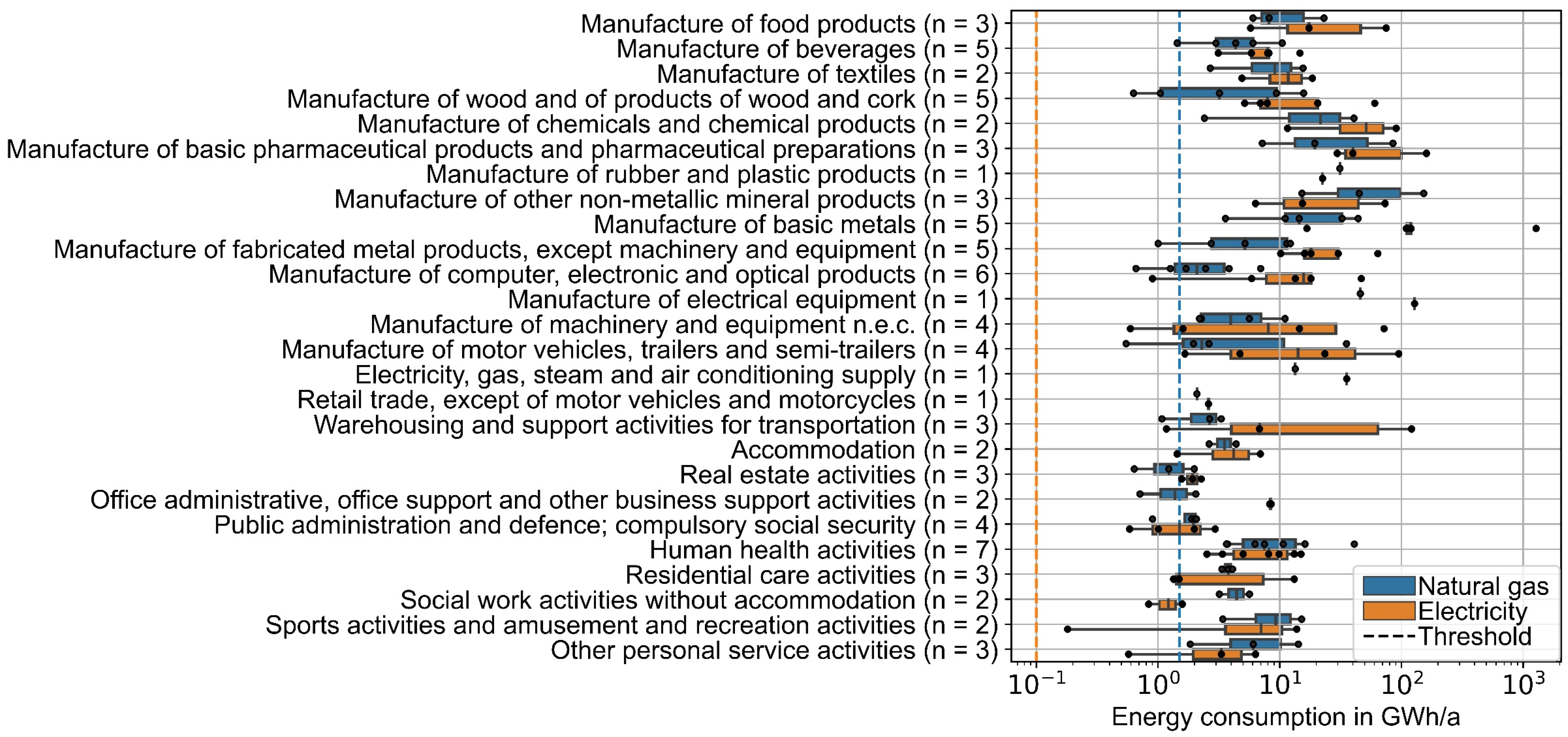
Table 1 provides an overview of the load profile database statistics, and
Figure 1 illustrates the distribution of the annual energy consumption in the 26 industry sectors for which load profiles are available. The energy consumption of most consumers is significantly higher than the thresholds for online measuring. However, the natural gas load of 12 consumers was measured online, although the annual consumption was less than 1.5 GWh/a. The highest energy consumption is observed in manufacturing industries. In all the manufacturing industries, except for the manufacture of other non-metallic mineral products, the electricity consumption is higher than natural gas consumption. In the tertiary sector, natural gas consumption is generally higher than electricity consumption.
The spread of energy consumption of the individual companies within the various industrial sectors is high. At the same time, the number of consumers in the individual industrial sectors is in the single digits. Furthermore, no additional information is available about the consumers, such as turnover or building size. Consequently, it is unreasonable to derive and compare any benchmarks on absolute energy consumption.
The 82 consumers in the load profile database are located in the German postal code regions 34 to 37. This covers the middle and northern part of Hesse and surrounding regions. Due to a lack of more detailed information on the consumers’ location, the same ambient temperature profile for all locations is used. This ambient temperature profile was measured at a weather station of the Hessian State Agency for Nature Conservation, Environment and Geology (HLNUG) in downtown Kassel, which is located approximately in the middle of the region from which the consumers originate.
3. Methods
This study compares five models for heat load profile prediction. Three models are taken from a previous study by the authors and are outlined in
Section 3.2. The only input features of these models are the type of day (wd or wknd) and the mean daily ambient temperature at the consumer’s location. These models are validated with the load profile database established for the present study (n = 82) and serve as a benchmark for evaluating the models developed in this study. Two models, one shallow learning and one deep learning model, are newly developed within this study. These models consider additional sources of information not previously evaluated. Electricity load is an input feature of both models. The deep learning model additionally evaluates time-lagged heat consumption.
For all models, a resolution of one day is applied. At this resolution, the correlation between heat demand and ambient temperature is clear. At higher resolutions, this correlation becomes unclear due to the thermal inertia of buildings. Therefore, established methods for predicting heat load profiles employ this resolution, e.g., the SLP method for the residential and commercial sector [
10]. At the same time, a resolution of one day is sufficient for most uses of load profile prediction methods mentioned above. For instance, as part of the preliminary design of renewable heating systems, the daily heat demand and fluctuating renewable energy sources must be balanced. To buffer imbalances at higher resolutions than one day, most renewable heating systems, such as solar thermal systems or heat pumps, can be equipped with storage. For example, solar thermal systems in industry are often equipped with a storage tank that can buffer the complete heat production on sunny summer days [
33]. Thus, a resolution of one day is sufficient for a first rough dimensioning of the plant capacity and a subsequent feasibility assessment. Only in detailed planning is the knowledge of a higher-resolution load profile necessary, e.g., to design the storage system. The same applies to anomaly detection. Variations of heat demand at a high resolution, e.g., hourly scale, do not necessarily indicate relevant anomalies but can have insignificant reasons, e.g., minor time shifts in the production process. In contrast, significant deviations of predicted and measured heat demand on the daily scale indicate serious system failures with higher accuracy. However, the resolution required in each case for the various applications of heat load profile prediction methods is not part of this study and must be determined in future studies on the respective applications.
In the further course of this section, pre-processing of the load profile database, model development, and model evaluation are outlined. Various Python-based software libraries are used for this study.
Appendix A gives an overview of the libraries and the version used in each case.
3.1. Pre-Processing
In the first pre-processing step, the resolution of the natural gas, electricity, and ambient temperature profiles is reduced to one day. In the next step, the load profiles are normalized. Natural gas load profiles are normalized on the mean daily consumption on days with a mean daily ambient temperature of 8 °C according to the SLP methodology [
10]. The choice of normalization temperature does not influence the qualitative results and is only a scaling factor. However, the chosen temperature corresponds approximately to the annual average temperature in Germany, so that it occurs frequently and the risk of normalization to an outlier is low. This methodology is explained in detail in the authors’ previous publication [
28]. The electricity load profiles are normalized on the maximum daily electricity consumption.
Natural gas consumption and heat demand are almost linearly correlated for standard boilers. Other technologies using natural gas are still very rare. For these reasons, this study assumes that normalized daily natural gas consumption is equal to normalized daily heat consumption. Due to the normalization, the natural gas boiler efficiency does not need to be considered. A detailed discussion of this assumption can be found in the authors’ previous work [
28].
To be used as input features for any of the tested machine learning algorithms, all numerical data (load and ambient temperature profiles) is standardized. Categorial data (day of the week) is one-hot encoded. For both standardization and one-hot encoding, the respective Scikit-Learn [
34] functions are used.
3.2. Model Development
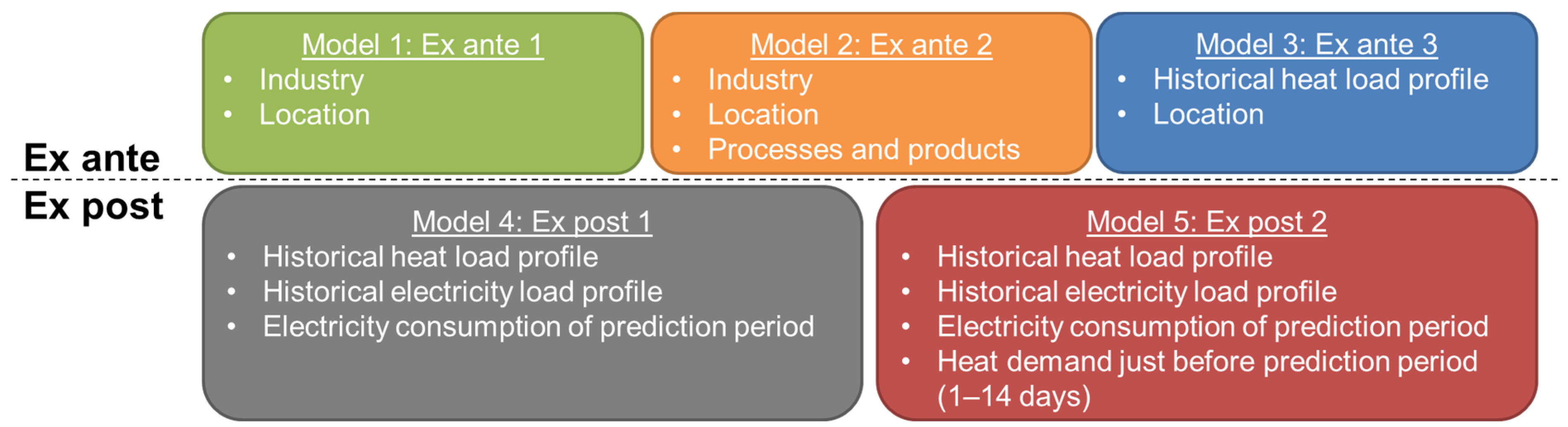
The five heat load profile models compared in this study can be distinguished by the amount of information they consider for the prediction.
Figure 2 provides an overview of the input features of each of the models. Models 1 to 5 consider successively more information. The three ex ante models are intended to predict the future heat demand, e.g., for preliminary design studies. Models 4 and 5 both consider the electricity consumption of the day when the heat demand is to be predicted. Consequently, only a prediction of the heat consumption for days in the past is possible (ex post). This limits the potential applications of these models. One potential application is automated anomaly detection in energy monitoring systems by comparing measured and predicted heat demand.
A representative ambient temperature profile is a required input of all models. For ex post prediction and training of all models, a measured ambient temperature profile of the same time span as the respective measured energy consumption profiles is used. If the ex ante models are used in practice, e.g., for feasibility studies, weather data from a test reference year (TRY) can be used. Alternatively, weather forecasts can be used for short-term heat demand prediction.
3.2.1. Ex Ante 1
In the authors’ previous study [
28], 797 annual load profiles with a resolution of one day are clustered according to their specific dependency on ambient temperature. For working days (wd), four clusters were defined (
Figure 3a). For weekends and holidays (wknd), five clusters were defined (
Figure 3b).
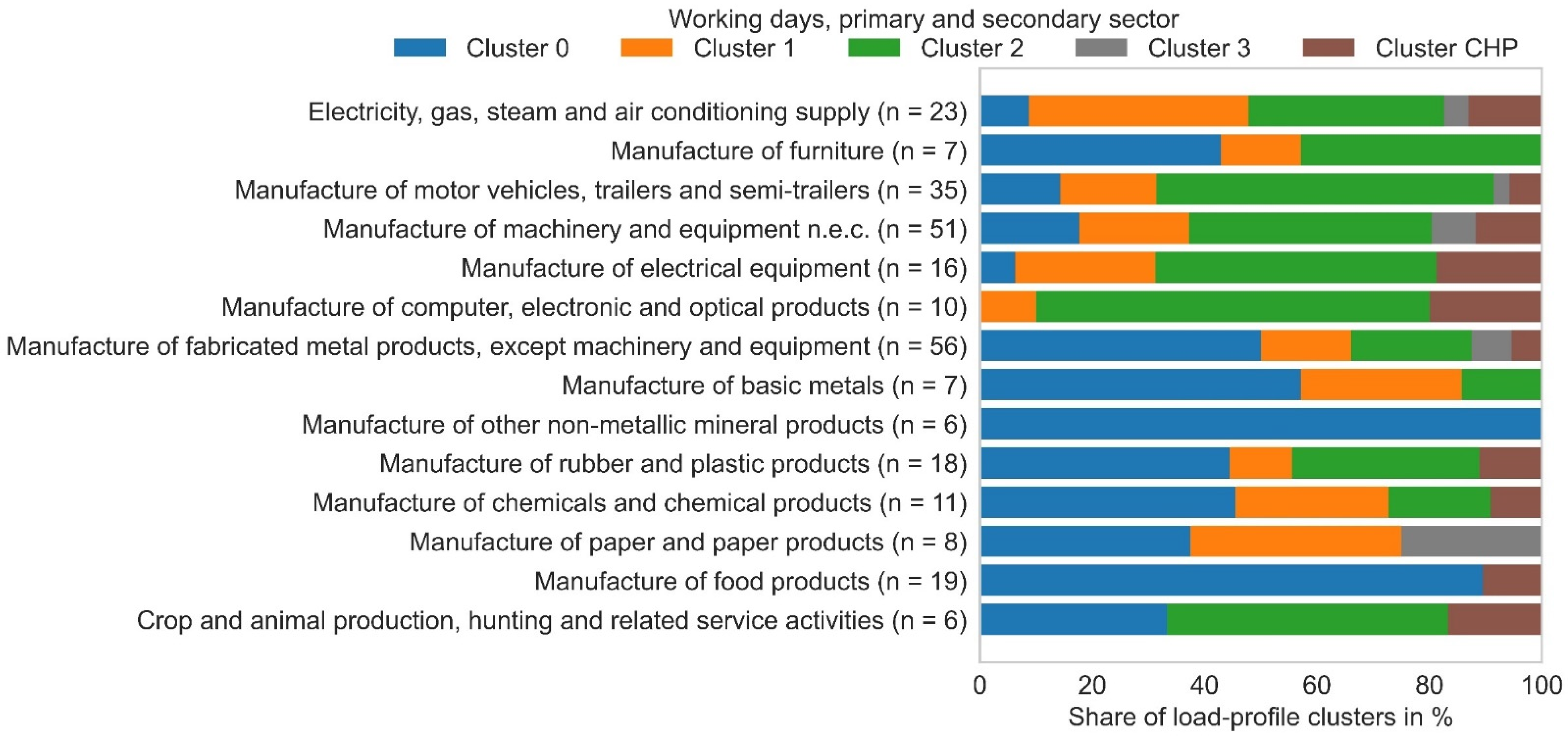
Figure 4 visualizes the frequency of each cluster within the different industry sectors [
28]. An important finding that can be seen from this figure is that the heat demand of most consumers depends on the ambient temperature, even in industry. There are only a few industry sectors in which wd-cluster 0, the cluster without dependence on ambient temperature, dominates. Consumers operating a combined heat and power plant (CHP) are not considered in the cluster analysis due to the possibility of a nonlinear relationship between natural gas consumption and heat demand.
In order to create a load profile for a particular consumer based on the results of the previous study, wd and wknd clusters must first be assigned to that consumer. For this purpose, the clusters that are most frequent in the industry of this consumer are selected (see
Figure 4 for a chart of wd frequencies for primary and secondary sectors or [
28] for tables on wd and wknd frequencies for consumers from all sectors). In the next step, the respective cluster regressions and a representative ambient temperature profile can be used to create a load profile (1) (see
Figure 3 for a diagram of cluster regressions and [
28] for tables on regression parameters). The regression function is composed of two linear functions. For ambient temperatures above the heating limit temperature (T
hl), a linear function represents the baseline heat demand in summer, e.g., due to water heating or other processes that are independent of the ambient temperature. For ambient temperatures below T
hl, a second regression line represents the heat demand, which increases linearly with decreasing ambient temperatures, e.g., due to space heating or heating processes that are dependent on the ambient temperature (drying, ventilation systems). Since wd and wknd-clusters are different, the heat demand must be calculated for wd and wknd separately [
28].
| y-axis intercept of space heating line (-) |
| y-axis intercept of domestic hot water (process heat) line (-) |
| slope of space heating line (-) |
| slope of domestic hot water (process heat) line (-) |
| normalized daily heat consumption (-) |
| daily mean ambient temperature (°C) (insert unitless) |
| heating limit temperature (°C) (insert unitless) |
3.2.2. Ex Ante 2
Since the ex ante 1 cluster assignment is based on frequencies only, cluster assignment errors are likely. In the previous work, the authors found that additional information on processes and products can be used to support a correct cluster assignment [
28]. One example for this is the cluster assignment in the manufacturing of furniture:
In this industry sector, the frequencies for the wd-clusters 0 and 2 are the same (
Figure 4). The product and process analyses of the seven companies in this industry reveal that the three consumers assigned to wd-cluster 0 manufacture furniture made of metal. They operate processes with a significant heat demand that is independent from ambient temperature, e.g., powder coating or surface treatment baths. In contrast, the three consumers assigned to wd-cluster 2 manufacture wooden furniture. They are not operating processes with a significant heat demand and space heating is their only relevant heat sink. Unfortunately, information on electricity consumption was not available for this earlier study by the authors.
The above example highlights the benefit of detailed information on a consumer’s products and processes for cluster assignment. However, this information is not available to this study. Therefore, an ideal cluster assignment is applied for the ex ante 2 model. This is done by determining the combination of wd and wknd-clusters that leads to the minimum sum of squared residuals between predicted and measured daily heat consumption of each consumer.
3.2.3. Ex Ante 3
The ex ante 3 model requires historical natural gas load profiles over a period of at least one year. These are used to fit the regression function (1) individually for each consumer. Similar to the previous models, one regression function is used for each wd and wknd.
3.3. Correlation of Heat and Electricity
This study investigates whether electricity load profiles can be used to optimize the heat load profile prediction. The idea behind this is that daily energy consumption could correlate with various other parameters that can be grouped under the umbrella term “user behavior”, e.g., utilization of production facilities, production times, vacation, or maintenance. For instance, an above-average utilization of production facilities could result in above-average daily electricity and heat consumption compared to other days with a similar ambient temperature and same type of day. The consequence would be a prediction of too-low consumption for such days by the ex ante models. A reason for the residuals of the ex ante models could therefore be that these models only consider the type of day (wd or wknd) and ambient temperatures but no user behavior. However, information on user behavior is not directly available for this study but may be derived from daily electricity consumption. Therefore, this study first investigates whether a correlation between daily electricity consumption and daily heat consumption can be verified. It is also reasonable to assume that electricity consumption is correlated to the residuals of the ex ante 3 model, which is also being investigated. Additionally, this study examines whether any of the above correlations are only stronger on weekdays or for groups of consumers assigned to one of the wd- or wknd-clusters. This correlation analysis is the basis for further load profile modeling.
3.3.1. Ex Post 1
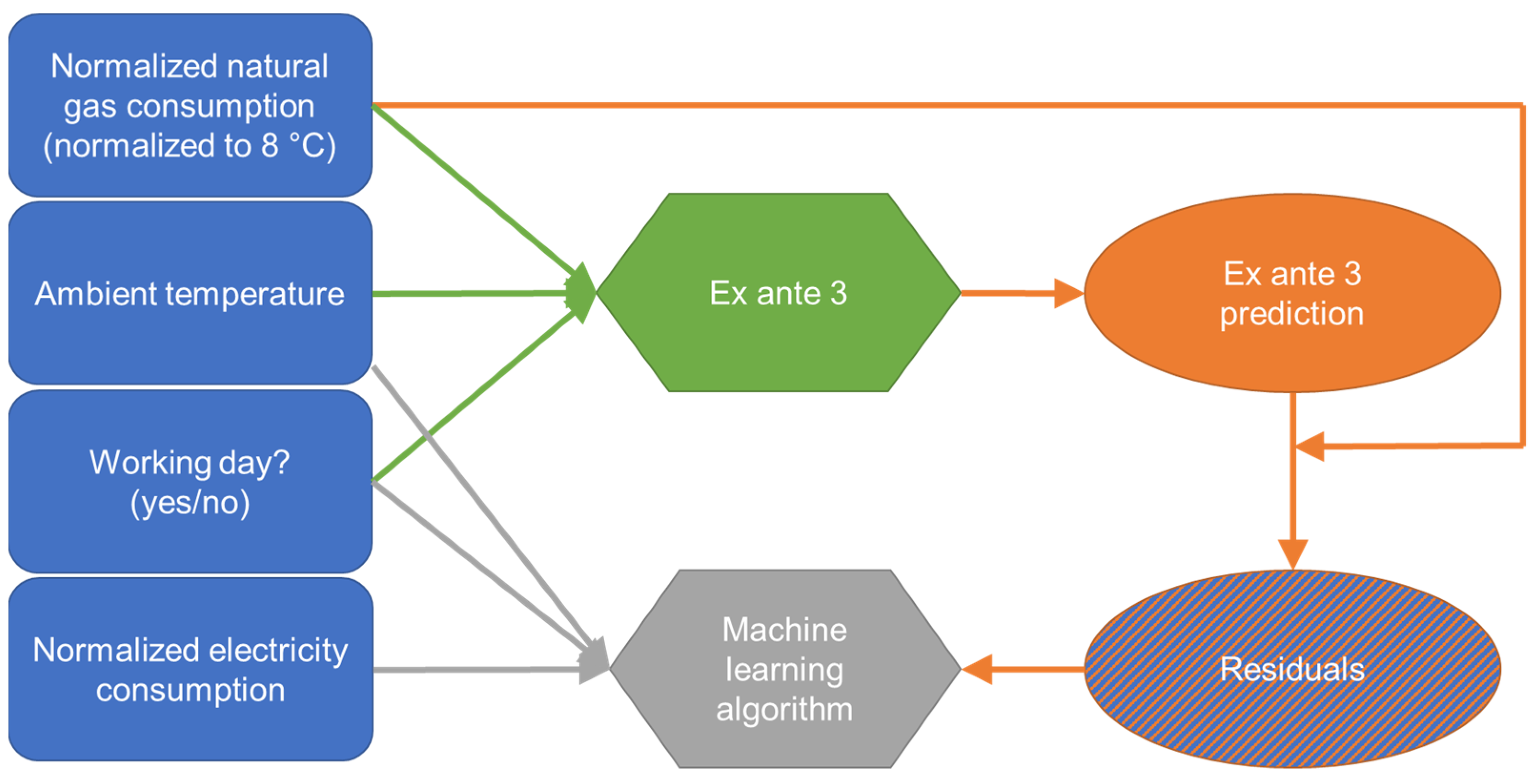
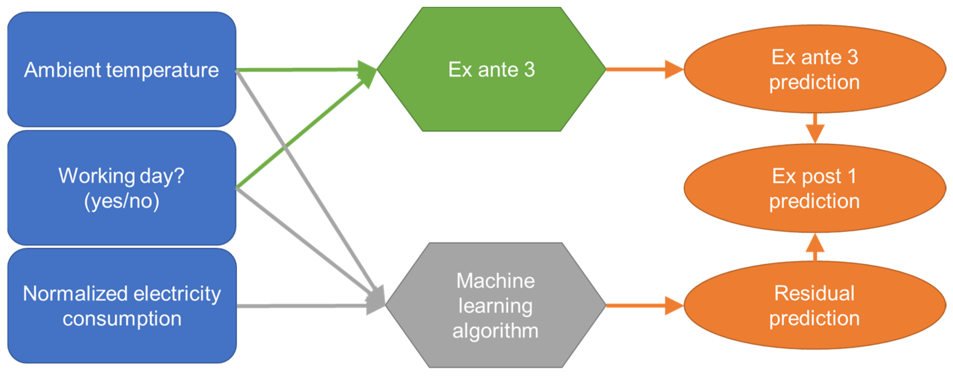
The ex post 1 model consists of two sub-models, so that the two models can be evaluated separately. The first sub-model corresponds to the ex ante model 3 and is intended to represent the influence of the ambient temperature on the heat demand. Since the heat demand is usually also affected by other influences, there are residuals between the ex ante 3 prediction and the actual heat demand. The second sub-model aims to predict these residuals, which are hypothetically mainly due to user behavior. To draw conclusions on user behavior, electricity consumption, type of day (wd or wknd), and ambient temperature are used as inputs of the second sub-model.
Figure 5 and
Figure 6 visualize the model architectures for training and prediction. As explained above, the residuals between the ex ante 3 prediction and the real heat demand are the intended result of the machine learning sub-model (residual predictions). Consequently, these residuals are used for supervised training of the machine learning algorithm (
Figure 5). When applying the final trained model, the residual predictions of the machine learning sub-model are used to improve the ex ante 3 model predictions (
Figure 6).
3.3.2. Ex Post 2
Load profiles are a sequence of observations that follow each other in time. It can be assumed that there is a relatively high similarity between observations that are close in time, but this relationship was not exploited by previous models. Arbitrarily changing the order of observations for training or prediction would not affect the results of the previous models. The ex post 2 model is intended to consider the sequence of the observations. For this purpose, lagged observations of the previous days’ heat demand are introduced as additional input features. To find the optimal time window of lagged observations, window lengths of 1 d, 2 d, 7 d and 14 d are compared. While the previous models only considered the type of day (wd or wknd), the ex post 2 model receives additional information about the day of the week. Due to time lagged heat consumption with a maximum of 14 values and a one-hot encoded type of day with 7 values, the number of input features of the ex post 2 model are significantly higher than in previous models. To ensure the model can benefit from this larger number of input features, a deep learning algorithm is selected for the ex post 2 model. The LSTM algorithm has proven to be one of the most advantageous deep learning algorithms for load profile modeling in literature and is therefore used in the ex post 2 model. Apart from the significantly increased number of input features and the more complex LSTM algorithm, the ex post 2 model architecture is simple compared to the ex post 1 model (
Figure 7).
Auto-Keras [
35] is used to create individual LSTM models for each consumer. The Auto-Keras base model consists of three blocks: The Input-block represents the input layer. An RNN-block embodies the hidden layers. A Regression-Head-block represents the output layer. The layer type of the RRN blocks is set to LSTM. All hyperparameters left unspecified are automatically tuned by Auto-Keras for each consumer individually, e.g., number of hidden layers and uni- or bidirectional architecture.
3.4. Evaluation of Correlations and Models
The dataset covers 82 natural gas and electricity load profiles for 2 complete years (2018 and 2019). First-year (2018) load profiles are used for training and second-year (2019) load profiles are used for model evaluation. This evaluation method corresponds to what is called “last block evaluation” in literature. Bergmeier and Benitéz [
36] presented a comprehensive review of cross validation methods for time series predictor evaluation. They conclude that last block evaluation tends to yield less robust error measures than cross-validation and blocked cross-validation. Nevertheless, last-block evaluation is used for the ex ante 3 to ex post 2 models for the following reasons:
Reduced computation time:
The overall sum of trained models in this study is high. For ex ante 3 to ex post 2, various regression algorithms are trained and compared with each other. Since this is done for each consumer individually, this results in a five-digit number of training runs. A more complex validation method, for example, a blocked cross-validation, would result in a higher number of training runs corresponding to the number of blocks.
Stationarity:
Bergmeier and Benitéz [
36] emphasized the importance of an adequate control for load profile stationarity before cross-validation. According to Cryer and Chan [
37], a load profile is stationary if the joint distribution
is the same as the joint distribution of
for all choices of time points
and all choices of time lag k. For annual natural gas load profiles with high seasonality, as examined in this study, the same distribution of two blocks is only given if both blocks cover at least a whole year. Only blocks of at least one year ensure that all occurring operation modes (e.g., normal operation, maintenance, holidays) are covered by each block.
Robust sample size:
For small sample sizes, accuracy metrics, such as R, can significantly deviate from the true value. Schoenbrodt and Perugini [
38] showed that a sample size of 362 is required to ensure an accuracy of R in the range of ±0.10 with a 90% confidence interval. This minimum sample size corresponds to the sample size used for the last-block evaluation (365 days). Cross-validation or blocked cross-validation with more than two blocks would result in smaller sample sizes and therefore less robust sample sizes.
The root mean square error (RSME) is used for model selection and training. Since RSME is an absolute value, it is not suitable for model comparison with other studies. Therefore, to evaluate the strength of the correlation between daily electricity consumption and daily heat demand or daily electricity consumption and ex ante 3 heat prediction residuals, the Pearson correlation coefficient (R) is used, which can range from −1 to 1. According to Cohen [
39], a strong correlation is characterized by an absolute value of R greater than 0.5. The sign of R indicates whether the respective values are positively or negatively correlated. If the correlation between two values is to be evaluated for a group of consumers, a median of approximately 0 could result, although only strong negative positive correlations are present. Therefore, whenever the strength of a correlation for a whole group of consumers is to be analyzed in this study, the coefficient of determination (R
2) is used. R
2 is usually defined to be between 0 and 1. Statistic parameters, such as the median or the quartiles of R
2, therefore evaluate the overall strength of a correlation for a group of consumers without considering their sign. The function to calculate R
2 implemented in Scikit-Learn [
34] and used in this study employs an alternative definition of R
2 (2) that can also lead to negative values if the sum of squared residuals is larger than the total sum of squares. However, negative values of R
2 are equally to be interpreted as zero values.
If the heat demand is constant throughout a period, R2 can still take values close to zero, even if the prediction is sufficiently accurate for the intended applications. Therefore, the standard deviation of the residuals (σ) is used as another metric for model accuracy evaluation.
| coefficient of determination (-) |
| SSR | sum of squared residuals (-) |
| SST | total sum of squares (-) |
| value (-) |
| mean of values (-) |
| prediction of values (-) |
4. Results
This section summarizes the results of the model development and evaluation. First, the ex ante models taken from a previous study are validated with the database of this study. In the next step, the results of the correlation analysis between electricity and heat consumption are outlined. This correlation is essential for the results of the ex post models described in the next section. Finally, the performance of all five models is compared.
4.1. Ex Ante Models
The cluster assignment based on the frequencies within each industry is only correct for 51% of wd-clusters and 54% of wknd-clusters according to the comparison of cluster identification in ex ante 1 and ex ante 2 if the ex ante 2 cluster identification is regarded as the correct cluster identification. This results in poor accuracy metrics for the ex ante 1 model (
Table 2). Improved cluster assignment for the ex ante 2 model and the individual linear regressions (ex ante 3) both result in significantly increased accuracy, which is at the same level for both models.
Figure 8 visualizes the distribution of R
2 for the ex ante 3 model separately for the four wd-clusters. The results of the other two ex ante models are similar, except that the overall accuracy of ex ante 1 is significantly poorer. For those consumers with a strong dependency on ambient temperature (wd-cluster 2 and 3), the ex ante model achieves a median of R
2 greater than 0.8. For wd-cluster 1, the cluster with only a small dependence on ambient temperature, the distribution of R
2 is much broader. For wd-cluster 0, the median of R
2 is at least 0.2 lower than the other clusters. The interquartile distance is two to three times higher than the other clusters.
4.2. Correlation of Heat and Electricity
The correlation between electricity and heat consumption varies strongly between the analyzed consumers (
Figure 9). For 41% of the consumers, a high positive correlation is detected (R > 0.5). Only 4% of the consumers show a high negative correlation (R < −0.5). For more than half of the consumers (55%), a low to medium correlation is discovered (−0.5 ≤ R ≤ 0.5). The mean R
2 is 0.33. Three examples of high, medium, and low correlation are presented below.
Figure 10 illustrates the electricity and heat consumption of an example consumer with a high correlation of both values. Heat and electricity consumption are significantly reduced on the wknd. The heat consumption shows only a slight seasonality, which can even be observed in the electricity load profile. When considering only weekdays or wknd days but also for the evaluation of the entire dataset, a clear correlation between electricity and heat consumption with R values larger than 0.9 is detected.
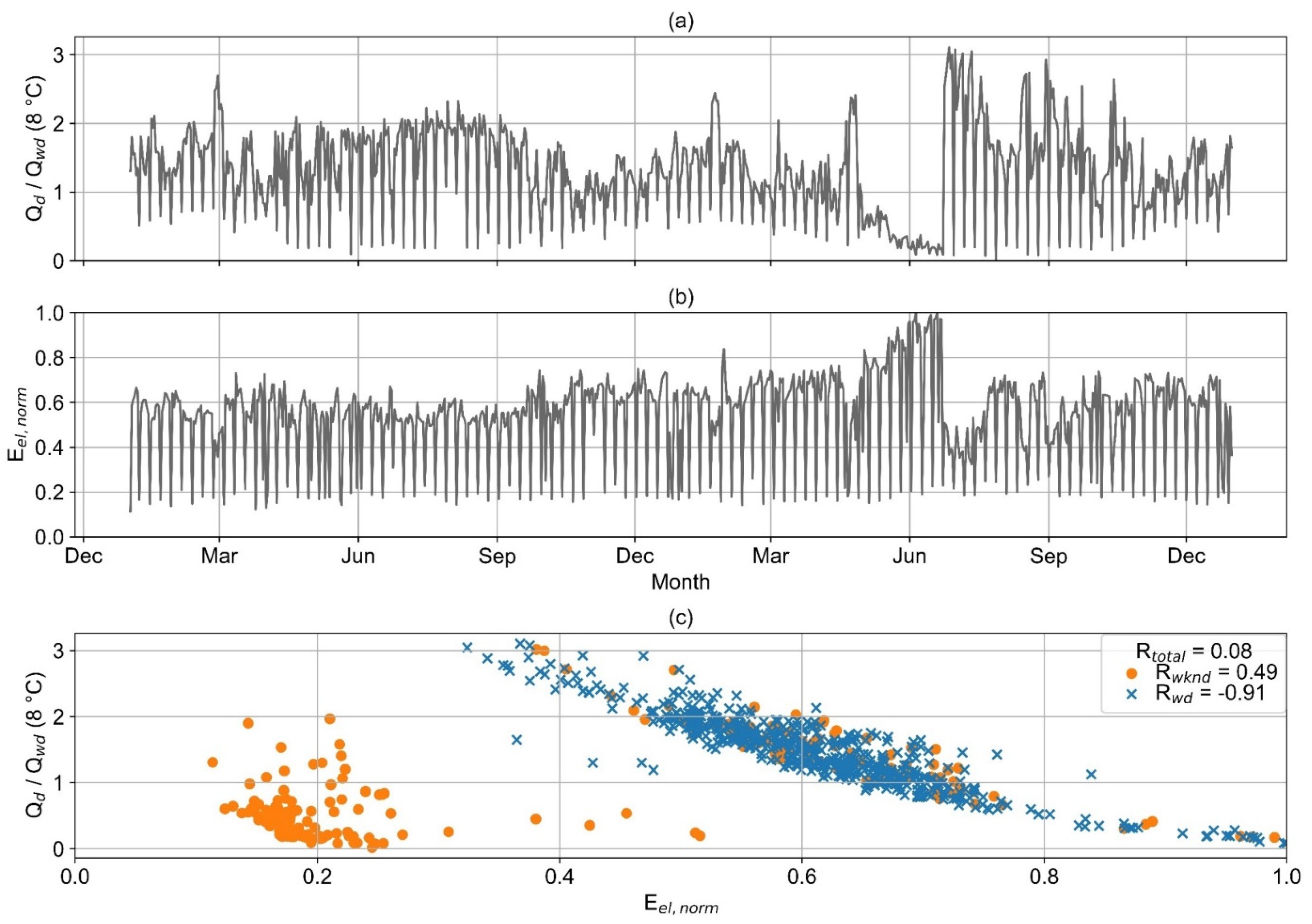
The value of R examined for the entire dataset of the second example consumer (wd and wknd) is very low (
Figure 11). Both heat and electricity consumption show no clear seasonality. For the wknd only, a medium correlation is detected (R
wknd = 0.49). The consumption of a few wknd days is in the range of wd. When only wd are considered, a high negative correlation can be detected (R = −0.91).
Figure 12 visualizes the load profiles of a consumer with a strong seasonality of their heat consumption. For about three months in the summer, there is absolutely no heat demand. In contrast, the electricity load profile shows no seasonality. As a result, the correlation between heat and electricity consumption is low. This applies for both the individual evaluation for wd or wknd, and for the evaluation of the entire dataset.
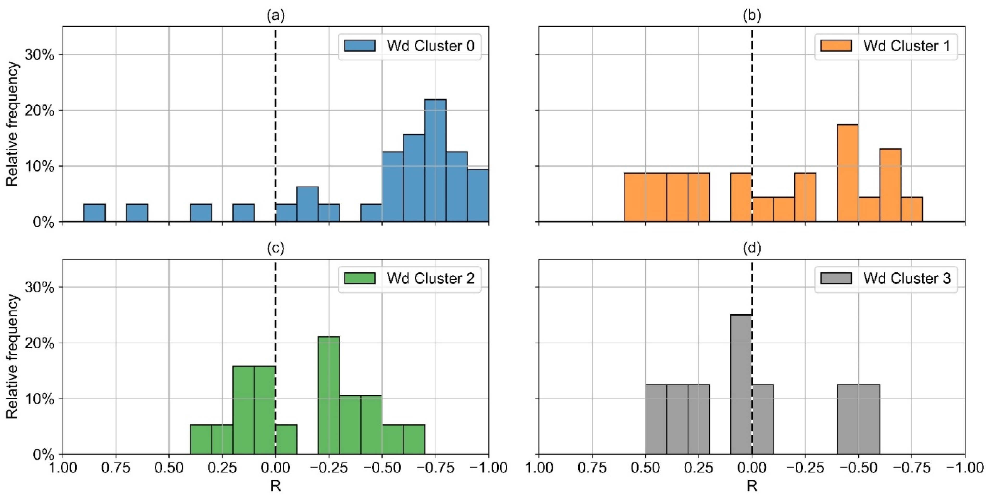
Due to different consumption patterns on wd and wknd, the correlation of heat and electricity consumption tends to be significantly higher for some of the consumers if wd and wknd are considered separately. Additionally, the correlation tends to be higher for consumers with a low seasonality in heat load profiles. For these reasons, histograms of R are shown in
Figure 13 for wd only and separately for the optimal wd-clusters.
The mean R2 only for wd is even slightly poorer than in general for all types of days (R2 = 0.33; R2wd = 0.28). In contrast, the correlation between electricity and heat consumption is significantly higher, if only non-seasonal consumers (wd-cluster 0) are considered (R2wd,cl 0 = 0.42). More than two thirds (69%) of the consumers in wd-cluster 0 show a strong correlation. For all other clusters, most consumers show a weak to medium correlation.
The seasonality of heat consumption is caused by the fluctuations of the ambient temperature during the year. This seasonality can be eliminated from the heat load profiles with the ex ante 3 model. The residuals between the ex ante 3 prediction and the actual heat consumption represent a heat load profile without the influence of ambient temperature. The distribution of R for the correlation of the ex ante 3 residuals and electricity consumption is illustrated in
Figure 14. Differences between
Figure 13 and
Figure 14 are small. The mean R
2 only for wd for all clusters is 0.26. If only consumers from wd-cluster 0 are considered, R
2 is 0.45.
4.3. Ex Post 1
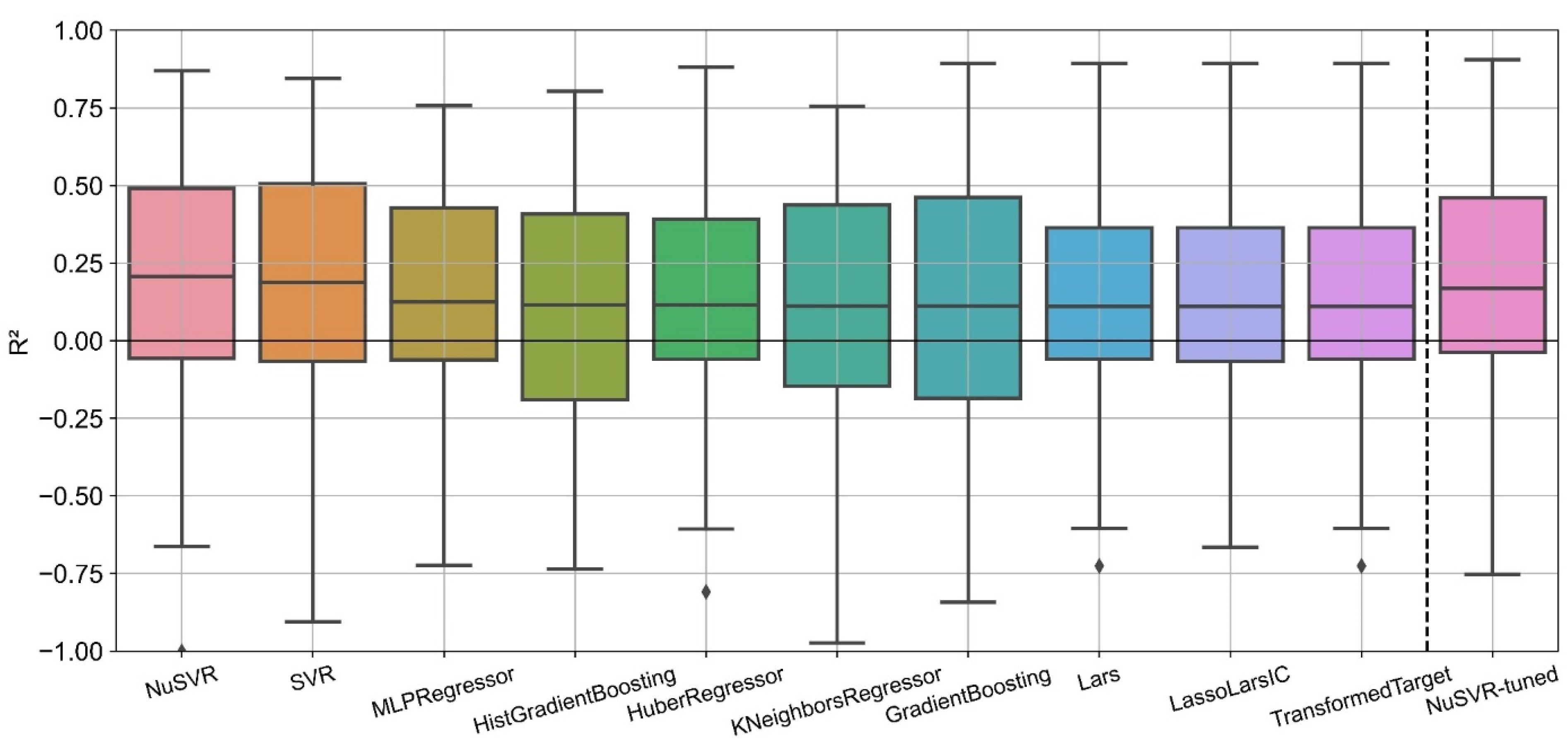
Figure 15 visualizes the distribution of R
2 for the residual prediction for 10 algorithms from Scikit-Learn with standard hyperparameters, which yield the highest median of R
2 for the 82 consumers examined in this study. For the algorithm with the highest median of R
2 (NuSVR), the plot also shows the distribution of R
2 after randomized hyperparameter tuning (NuSVR-tuned). Overall, differences between the algorithms are small. However, the variance of R
2 for each algorithm between the 82 consumers is large. For each of the algorithms, R
2 ranges roughly from −1.0 to 0.8. Negative R
2 values occur when the sum of squared model residuals is larger than the total sum of squares (see
Section 3.4). With standard hyperparameters, NuSVR yields the highest median of R
2. Therefore, the NuSVR algorithm is selected to be optimized but the randomized hyperparameter tuning of the NuSVR algorithm (NuSVR-tuned) does not lead to a significant improvement. While the maximum R
2 and the lower quartile are slightly increased, the upper quartile and the median of the tuned NuSVR algorithm are poorer than of the standard NuSVR algorithm.
Figure 16 visualizes the distribution of R
2 of the NuSVR residual prediction separated by the different clusters. Only for the wd-clusters 0 and 1, R
2 values of more than 50% are achieved. This corresponds to the results of the correlation analysis (
Figure 14). Consumers from these clusters, especially from wd-cluster 0, show by far the strongest correlations between heat consumption and ex ante 3 residuals.
For wd-cluster 2 and 3, the ex post 1 prediction results are almost identical to the ex ante 3 results (
Figure 8 and
Figure 17). For wd-cluster 1 and especially wd-cluster 0, the overall prediction accuracy is significantly improved. The distribution of R
2 is narrower and shifted towards higher values. For all wd-clusters, the median of R
2 is greater than 0.8.
R
2 of the ex post 1 sub-model’s residual prediction is below 0.5 for more than 75% of the consumers, but the complete ex post 1 model only leads to a poorer heat prediction for 13% of the consumers, compared to the ex ante 3 model (
Figure 18). However, for most consumers, only small improvements of less than 5 percentage points of σ and R
2 are observed. On average, σ is improved by 4 percentage points and R
2 by 12 percentage points. The maximum decrease in σ and R
2 is 3 percentage points and 5 percentage points, respectively.
4.4. Ex Post 2
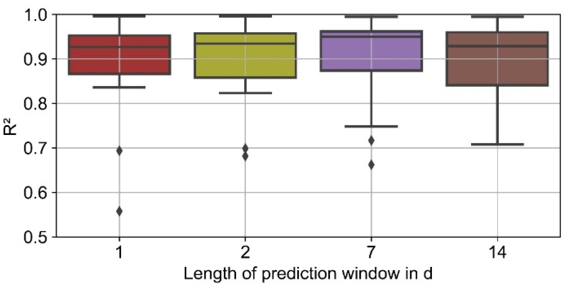
The differences between the results for the analyzed window lengths for lagged heat consumption are small (
Figure 19). Overall, a window length of 7 days leads to the highest quartiles and highest median of R
2, but to a slightly poorer minimum prediction accuracy compared to a window length of 2 days or 14 days.
For all consumers assigned to wd-clusters 1 to 3 except for 1, R
2 of the ex post 2 prediction is larger than 0.8 (
Figure 20). For most of these consumers, R
2 is even larger than 0.9. The distribution of R
2 is broader for wd-cluster 1. With one exception, however, for all consumers from wd-cluster 0, the R
2 is greater than 0.6.
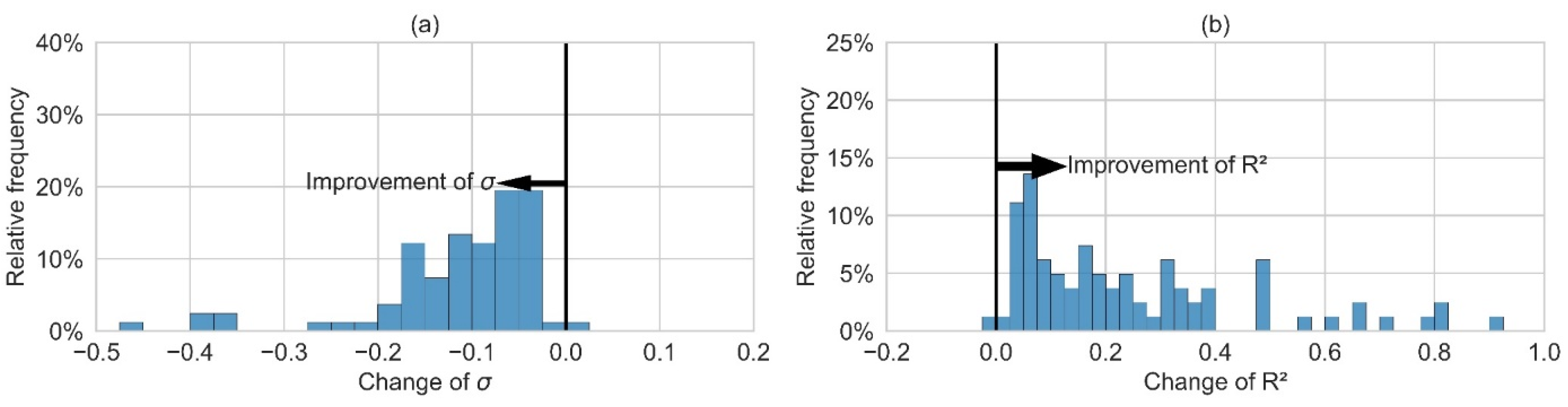
Compared to the ex ante 3 model, the ex post 2 model leads to an improvement for all but one consumer (
Figure 21). The range of improvement is broad. Again, for many consumers the improvement is small, with changes of σ and R
2 of about 5 percentage points. For most consumers, the improvement is in the range of up to 20 percentage points of σ or 40 percentage points of R
2.
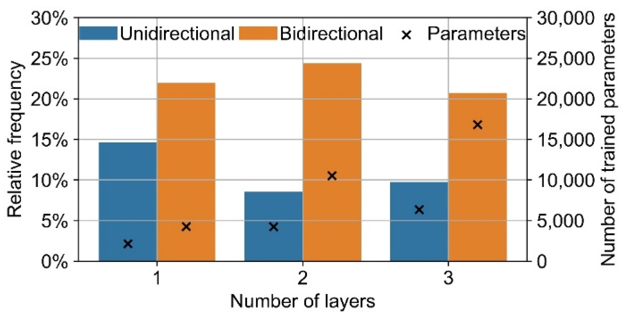
The optimization of the number of layers and layer type in Auto-Keras leads to varying LSTM architectures (
Figure 22). The depth ranges from one to three layers and is almost equally distributed. Two thirds of the models are bidirectional.
4.5. Model Comparison
The residual distribution of all models is unbiased (
Figure 23). From ex ante 1 to ex post 2, σ is successively reduced. Substantial improvement occurs especially from ex ante 1 (σ = 43%) to ex ante 2 (σ = 32%) and from ex post 1 (σ = 27%) to ex post 2 (σ = 17%). The residual distribution of ex ante 2 and 3 is almost the same. The ex ante 3 model has a slightly more pronounced peak at around 0, but also some stronger outliers, which results in almost the same σ for ex ante 2 and 3 (σ = 32%).
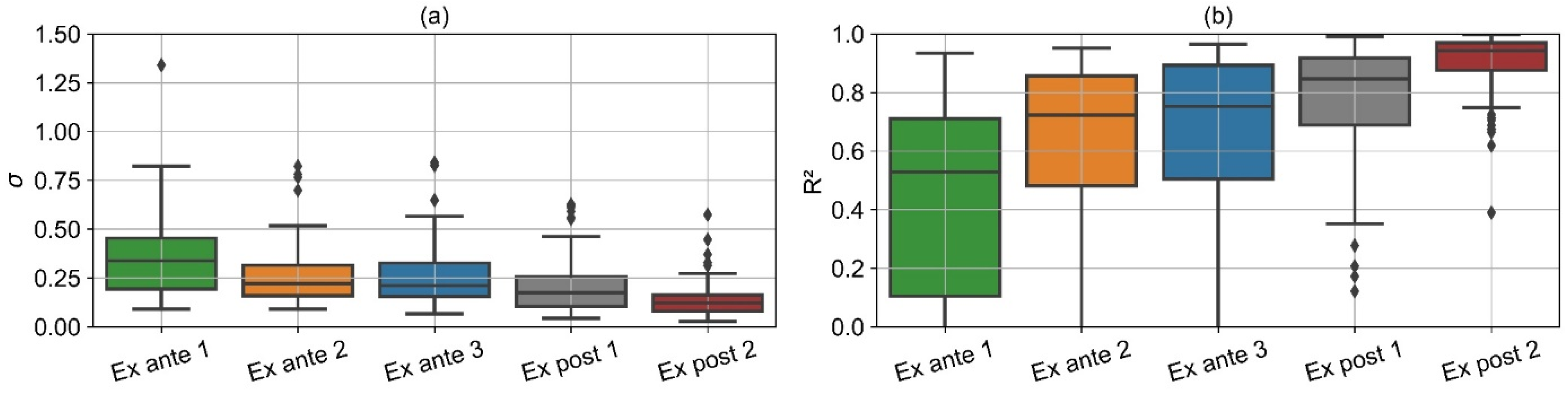
Figure 24 illustrates individual σ (a) and R
2 (b) values of each consumer. The distribution of both metrics is successively improved from ex ante 1 to ex post 2. While the improvement from ex ante 1 to ex post 1 is smooth, the ex post 2 model stands out clearly, especially in reducing poor predictions. R
2 of all models except ex post 2 ranges from negative values (not shown in
Figure 24) to about 0.9. In contrast, R
2 is below 0.6 only for one consumer for the ex post 2 model.
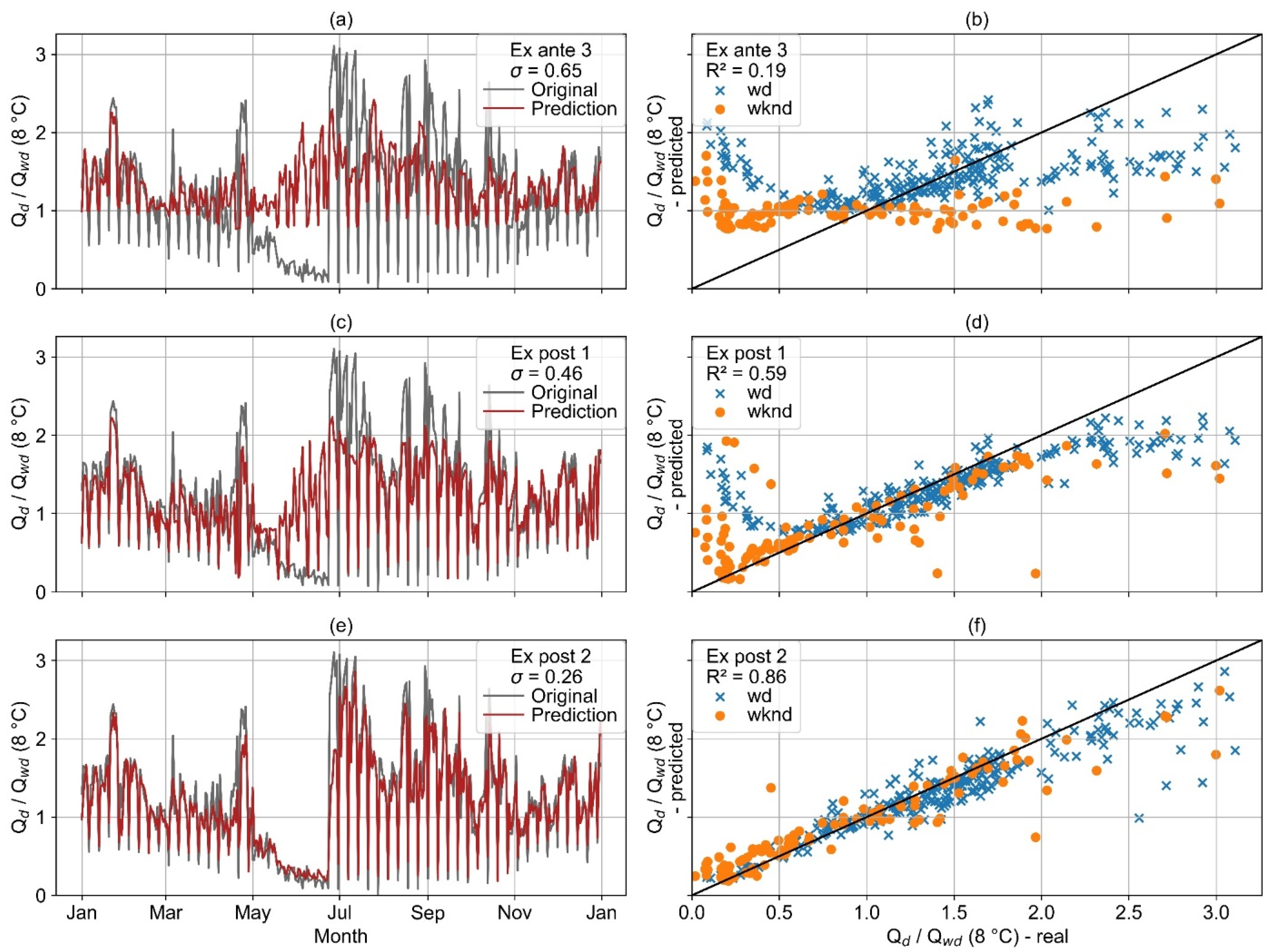
Figure 25 visualizes the actual and predicted load profiles for example consumer 1, which is characterized by a strong correlation between heat and electricity consumption. The consumer is the same as illustrated in
Figure 10. Overall, high accuracy is achieved with all models. However, the ex ante 3 prediction for wd does not correctly reflect the actual trend, but this does not have a strong negative impact on R
2 due to the overall relatively small fluctuations in heat consumption.
Figure 26 illustrates the actual and predicted load profiles of example consumer 2, which has a strong negative correlation on wd and a medium correlation on wknd (
Figure 11). Ex ante 3 and ex post 1 both fail to predict the collapse of the heat consumption from May to July and the peaks of heat demand from July to November. However, the prediction of the ex post 1 model better approximates the real load profile overall. In contrast to the ex ante 3 and ex post 1 models, the ex post 2 model predicts both types of events much better.
The actual and predicted load profiles of example consumer 3 are illustrated in
Figure 27. This consumer does not show a correlation between heat and electricity consumption (
Figure 12). The ex ante 3 and ex post 1 model both result in a significant underprediction of heat consumption during most time of the year and a minor over-prediction in the summer. In contrast, the ex post 2 model results in a highly accurate prediction for the whole year.
5. Discussion
This section presents a discussion of the results outlined above. First, the results of each model and the correlation analysis are evaluated separately. In the next step, the differences between the five models are reviewed.
5.1. Ex Ante Models
The accuracy of the ex ante 1 model is poor compared to the other models, especially for wd-cluster 0. Since the cluster assignment is correct for only about 50% of wd- and wknd clusters, many predicted load profiles significantly differ from the real load profiles. In their previous work [
28], the authors revealed that the cluster assignment based on the most probable cluster in the consumer’s industry sector can be optimized with expert knowledge and information about the consumer’s processes and products. Since the consumers in this study are anonymized, this method cannot be applied. To simulate the optimization of the cluster assignment by the ex ante 2 model, the optimal clusters are derived from first year’s data. The accuracy of the ex ante 2 model is significantly higher than that of the ex ante 1 model.
The ex ante 3 model uses individual linear regressions for each consumer. Similar to the authors’ previous work, individual regressions (ex ante 3) are only slightly more accurate than the optimal cluster regressions (ex ante 2).
In their previous work, the authors filter the load profile database and exclude load profiles for different outlined reasons. For example, load profiles are excluded that are obviously incomplete, where obvious anomalies occur, e.g., due to long maintenance shutdowns, or where CHP plants are operated. In contrast, this study’s load profile database is not filtered. This study’s load profile database contains some very unusual load profiles with conspicuous anomalies, which is evident from the visualizations in the
supplementary materials [
40]. These unusual load profiles explain why the overall accuracy of both ex ante 2 and 3 models is below that of the authors’ previous study [
28]. However, R
2 is still higher than 0.7 for the majority of the consumers. Especially for those consumers strongly dependent on the ambient temperature (wd-clusters 2 and 3), the overall accuracy is sufficient for less demanding applications, such as preliminary design studies. In contrast, strong unexplained variances in heat load often occur for consumers from wd-clusters 0 and 1, making the ex ante models less applicable for these consumers.
5.2. Correlation of Heat and Electricity
The patterns of the respective correlations between heat and electricity consumption are extremely heterogeneous for the consumers studied. This is evident not only in the statistical analysis of R and the 3 consumer examples above, but also in the
supplementary materials [
40] that contains plots of the heat and electricity load profiles of all 82 consumers in the style of
Figure 10,
Figure 11 and
Figure 12. Some consumers show strong negative or positive correlations, but for most consumers, weak to medium correlations were detected. The situation is different if only consumers without seasonal heat consumption are considered (wd-cluster 0). These consumers have an almost constant heat consumption on wd over the year. No information about the consumer’s heat sinks is available, but the constant heat demand can hypothetically be explained by a high proportion of process heat demand that is independent of the ambient temperature. Space heating seems to be secondary for these consumers. It can be assumed that both process heat and electricity consumption are strongly influenced by user behavior, which explains why both values are strongly correlated for consumers assigned to wd-cluster 0. In contrast, the consumption of wd-clusters 2 to 3 is dominated by space heating, which is mostly dependent on ambient temperature and only marginally on user behavior. This explains why only weak to medium correlations between heat and electricity consumption can be detected for most consumers from wd-clusters 2 to 3. Wd-cluster 1 is a hybrid cluster. This cluster shows a distinct dependence on ambient temperature. At the same time, roughly a third of the consumers show a strong correlation between heat and electricity consumption.
No parameter is identified that indicates the pattern of the respective correlation. The largest part of the consumers in wd-cluster 0 shows a strong correlation. However, the pattern of the relationship between heat and electricity consumption still varies strongly. Consequently, all models that consider electricity consumption for load profile prediction are trained individually for each consumer with historical data of that consumer. Therefore, if electricity consumption is to be used for the prediction of heat load profiles, the use of generally transferable models that do not need to be trained individually for each consumer, such as the models ex ante 1 and 2, is not reasonable.
5.3. Ex Post 1
No shallow learning algorithm could be identified in literature that clearly stands out for load profile modeling. This corresponds to the results of this study. The top 10 of the examined shallow learning algorithms lead to similar residual prediction results.
The ex post 1 sub-model for residual prediction only yields satisfying results if a strong correlation between electricity consumption and ex ante 3 residuals exists. This is only the case for a relevant share of the consumers assigned to wd-cluster 0. For most consumers from wd-cluster 1 and all other consumers from wd-clusters 2 and 3, residuals cannot be predicted based on the used input features and the examined shallow learning algorithms. Despite the overall poor accuracy of the residual prediction, the complete ex post 1 model is superior to the ex ante 3 model. A deterioration in prediction accuracy only occurs to a small extent for a few consumers. For most consumers, the prediction is only slightly increased. However, for those consumers where there is a strong correlation between heat and electricity consumption, a significant improvement can be achieved. This is evident by the significant improvement of the heat load prediction for consumers from wd-cluster 0.
5.4. Ex Post 2
A seven-day window of lagged heat consumption leads to the best results and is therefore selected for the present study. This could be explained by the assumption that the heat consumption on the same days of the week is more correlated than on different days of the week. A seven-day window length is just long enough to include the same weekday from the last week. The longer the time window becomes, the less the values are closely related in time, which could explain poorer results for a 14-day window.
The model architecture varies for the examined consumers. This suggests that not all input features are equally relevant to different consumers or that the relationships between inputs and outputs are not equally complex. For example, many consumers do not show a correlation between heat and electricity consumption, which reduces the number of relevant input features and could be an explanation for more shallow architectures for these consumers.
The prediction accuracy of the ex post 2 model is the highest even for consumers from wd-clusters 1 to 3, whose load profiles depend on the ambient temperature. For these consumers, the overall high prediction accuracy suggests that the input features cover all relevant parameters. In contrast, the prediction accuracy is below 0.8 for more than a quarter of the consumers in wd-cluster 0. These consumers are not dependent on ambient temperature. Additionally, a third of these consumers show only a weak correlation between heat and electricity consumption. The remaining input features (weekday and lagged heat consumption) do not include enough information to predict the heat demand with the same accuracy as achieved for almost all consumers in one of the other clusters. However, no additional information about the consumers is available to this study and the prediction accuracy can therefore not be increased for these consumers.
5.5. Model Comparison
Regular heat load profiles, which are mainly influenced by the ambient temperature, can be predicted by all models with a high accuracy. When ambient temperature is insufficient to explain most of the variation of a heat load profile of a specific consumer, electricity consumption and lagged heat consumption have proven to be useful sources of information to draw conclusions about other influences, such as user behavior.
Especially for consumers from wd-cluster 0, the ex post 1 model achieves clear improvements compared to the ex ante models. For most consumers from wd-cluster 0, the heat demand is correlated to the electricity consumption. This correlation is used by the ex post 1 model to optimize the prediction accuracy. For many consumers, however, the electricity consumption used as input feature is not correlated with the output value heat consumption. This leads to poor results of the ex post 1 residual prediction sub-model, especially for wd-cluster 2 and 3. For some consumers, this poor residual prediction, in turn, leads to a minor degradation of the complete ex post-1 prediction.
A major advantage of the ex post 2 model over the ex post 1 model is that all input features are automatically weighted. Irrelevant input features, which could lead to a deterioration of the results, are automatically ignored. Additionally, the ex post 2 model also uses lagged heat consumption to draw conclusions about other influences on heat demand, such as user behavior. In combination, this enables the ex post 2 model to achieve significant improvements over all other models, even for consumers that show no correlation between heat and electricity consumption.
The advantages of the ex post models are made clear by the three presented example consumers. For consumer 1 (
Figure 10 and
Figure 25), the wknd heat consumption is almost constant over the year and only minorly influenced by the ambient temperature. Consequently, all models achieve a high prediction accuracy for wknd. In contrast, the wd heat consumption is not only influenced by the ambient temperature. Only because the overall variation in wd heat consumption is relatively small does the ex ante 3 model still achieve a satisfactory accuracy. Since the electricity and heat consumption of example consumer 1 are strongly correlated (
Figure 10), which is typical for consumers from wd-cluster 0, both ex post models achieve highly accurate results.
The heat load profile of example consumer 2 (
Figure 11 and
Figure 26) shows strong anomalies that cannot be predicted by the ex ante models. Based upon the medium to high correlation of electricity and heat consumption (
Figure 11), both ex post models achieve better results than the ex ante models. Nevertheless, the ex post 1 model still fails to predict the anomalies. In contrast, the ex post 2 model achieves a high accuracy for the whole year. However, it is noteworthy that the ex post 2 model also initially makes incorrect predictions at the beginning of the anomalies. Only a few days later, when the anomaly also becomes clear in the lag observations, is it correctly predicted.
The ex ante 3 and ex post 1 models both fail to predict the heat consumption of example consumer 3 (
Figure 12 and
Figure 27) correctly. This can be explained by a major change of the heat consumption pattern from the training year’s data to test the year’s data of this consumer. Based on lagged consumption, this shift is detected by the ex post 2 model, which leads to the significantly better prediction results of this model compared to the rest of the models.
6. Conclusions
The most accurate possible prediction of heat load profiles with a resolution of one day is essential for many applications in the context of the energy transition. Recently, the need to accelerate energy efficiency and renewable energy projects due to global crises, such as the war in Ukraine, has further increased the demand for accurate load profile prediction methods. Previous heat load profile models are accurate for consumers dominated by ambient temperature dependent heat demand, e.g., space heating. However, previous models fail to predict the heat demand of consumers with a high share of ambient temperature independent (process) heat demand. In contrast, this study develops models that are highly accurate for all types of consumers from industry and the tertiary sector based on a database of measured load profiles from 82 German consumers from industry and the tertiary sector.
Ambient temperature independent (process) heat demand is affected by influences including utilization of production facilities, production times, vacation, or maintenance, which can be grouped under the term “user behavior”. To predict the user behavior-influenced part of heat demand correctly, this study uses the electricity consumption as an input feature. For most consumers with a high proportion of ambient temperature-independent (process) heat demand, there is a clear correlation between heat and electricity consumption. In contrast, for consumers whose heat demand depends on the ambient temperature, there is usually no correlation between heat and electricity consumption.
This study develops two model architectures, one shallow and one deep learning. With a median of R
2 of 0.84, the NuSVR algorithm showed slight advantages in overall accuracy compared to 51 other shallow learning algorithms from the Python-based Scikit-Learn library [
34]. Based on the literature review, the LSTM algorithm is selected for the deep learning model. In addition to electricity consumption, the LSTM algorithm also evaluates the heat consumption of the last 7 days prior to the predicted day and achieves by far the highest accuracy with a median of R
2 of 0.94.
The pattern of the correlation between heat and electricity consumption is user specific. Therefore, the developed models are trained for each consumer individually with measured load profiles from the past. The LSTM model architecture (number of layers, unidirectional or bidirectional) is also adapted individually for each consumer. In contrast, to apply previous models, only the information about a specific consumer’s industry and a representative ambient temperature profile is required. Thus, the higher accuracy of the models developed in this study is accompanied by higher data availability requirements and a more complex application. Possible applications are, e.g., automated anomaly detection in energy monitoring systems.
7. Directions of Future Work
The model architectures chosen are justified but represent only an initial proposal to evaluate the potential of machine learning-based prediction of heat load profiles based on commonly available information, such as electricity consumption. Depending on the intended application, the combination of optimal input features and machine learning algorithms should be examined more closely. It would also be conceivable, for example, to develop a model that makes an ex ante prediction based on a weather forecast and the electricity and heat consumption of the last few days, e.g., for model predictive control.
Since all required input features are usually available to consumers connected to public natural gas and electricity grids, or operating an energy monitoring system, and due to the achieved high accuracy, the ex post 2 model is assumed to be suitable for automated anomaly detection in energy monitoring systems. However, this study did not investigate the actual integration into energy monitoring systems, which was not possible based on the anonymized load profile database. For this purpose, a non-anonymized database with extensive information on the consumers would be necessary, to distinguish between normal operation and anomalies. Based on such a database, the anomaly detection algorithm could be developed, for which several approaches are conceivable:
If the difference of actual and predicted load profile exceeds a defined threshold, an anomaly is indicated. This threshold must be determined.
Only one classification algorithm uses the same inputs as the ex post 2 model and additionally evaluates the actual heat consumption.
A two-step algorithm first uses the ex post 2 model to predict heat consumption. In the next step, another algorithm could detect an anomaly based on actual and predicted heat consumption.
Author Contributions
M.J.: conceptualization, methodology, writing—original draft. F.P.: funding acquisition, project administration, writing—review and editing. K.V.: funding acquisition, supervision. U.J.: writing—review and editing, supervision. All authors have read and agreed to the published version of the manuscript.
Funding
This work was supported by the German Federal Ministry for Economic Affairs and Climate Action within the framework of the 7th Energy Research Program [project: “AnanaS”, grant number 03ETW014A].
Institutional Review Board Statement
Not applicable.
Informed Consent Statement
Not applicable.
Data Availability Statement
The original and normalized load profile database examined in this study cannot be published for data protection reasons. Measured weather data is available from Hessian State Agency for Nature Conservation, Environment, and Geology [
41].
Acknowledgments
The authors would like to express their sincere thanks to the involved utility for providing natural gas and electricity load profiles.
Conflicts of Interest
The authors declare no conflict of interest. The funders had no role in the design of the study; in the collection, analyses, or interpretation of data; in the writing of the manuscript, or in the decision to publish the results.
Nomenclature
| ANN | artificial neural network |
| b | y-axis intercept (-) |
| CHP | combined heat and power |
| HLNUG | Hessian State Agency for Nature Conservation, Environment, and Geology |
| HVAC | heating, ventilation, and air conditioning |
| k | time lag (d) |
| lin | linear |
| m | slope (-) |
| MAE | mean absolute error |
| MPC | model predictive control |
| n | number (-) |
| Q | natural gas consumption, heat demand (kWh) |
| R | Pearson correlation coefficient (-) |
| R2 | coefficient of determination (-) |
| RSME | root mean square error (-) |
| SLP | standard load profile |
| SSR | sum of squared residuals (-) |
| SST | total sum of squares (-) |
| SVM | support vector machines |
| T | temperature (°C) |
| TRY | test reference year |
| wd | working day |
| wknd | weekends and holidays (idle days) |
| XGBoost | extreme gradient boosting |
| y | value |
| mean of values |
| ŷ | prediction of value |
| Greek symbols |
| σ | standard deviation (-) |
| Subscripts |
| amb | ambient |
| d | day, daily |
| h | (space) heating |
| hl | space heating limit |
| w | hot water or process heat |
| wd | working day |
| wknd | weekends and holidays (idle days) |
Appendix A
Table A1.
Python software libraries and versions used in this study.
Table A1.
Python software libraries and versions used in this study.
| Library | Version | Reference |
|---|
| Auto-Keras | 1.0.12 | [35] |
| Keras | 2.4.3 | [42] |
| Matplotlib | 3.2.2 | [43] |
| Numpy | 1.19.1 | [44] |
| Pandas | 1.1.3 | [45] |
| Python | 3.8.5 | [46] |
| Scikit-Learn | 0.23.2 | [34] |
| Scipy | 1.5.0 | [47] |
| Seaborn | 0.11.0 | [48] |
References
- IEA. A 10-Point Plan to Reduce the European Union’s Reliance on Russian Natural Gas. 2022. Available online: https://iea.blob.core.windows.net/assets/1af70a5f-9059-47b4-a2dd-1b479918f3cb/A10-PointPlantoReducetheEuropeanUnionsRelianceonRussianNaturalGas.pdf (accessed on 25 March 2022).
- Hoang, A.T.; Sandro, N.; Olcer, A.I.; Ong, H.C.; Chen, W.-H.; Chong, C.T.; Thomas, S.; Bandh, S.A.; Nguyen, X.P. Impacts of COVID-19 pandemic on the global energy system and the shift progress to renewable energy: Opportunities, challenges, and policy implications. Energy Policy 2021, 154, 112322. [Google Scholar] [CrossRef] [PubMed]
- Lauterbach, C. Potential, System Analysis and Preliminary Design of Low-Temperature Solar Process Heat Systems. Ph.D. Thesis, Kassel University Press, Kassel, Germany, 2014. [Google Scholar]
- Wolf, S. Integration of Heat Pumps into Industrial Production Systems: Potentials and Instruments for Tapping Potential. Ph.D. Thesis, Universität Stuttgart, Stuttgart, Germany, 2017. (In German). [Google Scholar]
- Afroz, Z.; Shafiullah, G.M.; Urmee, T.; Higgins, G. Modeling techniques used in building HVAC control systems: A review. Renew. Sustain. Energy Rev. 2018, 83, 64–84. [Google Scholar] [CrossRef]
- Ordinance on Access to Electricity Supply Networks: StromNZV. 2021. Available online: https://www.gesetze-im-internet.de/stromnzv/StromNZV.pdf (accessed on 25 March 2022). (In German).
- Gas Network Access Ordinance: GasNZV. 2019. Available online: https://www.gesetze-im-internet.de/gasnzv_2010/GasNZV.pdf (accessed on 25 March 2022). (In German).
- Act on Metering Point Operation and Data Communication in Intelligent Energy Networks: MsbG. 2021. Available online: https://www.gesetze-im-internet.de/messbg/MsbG.pdf (accessed on 25 March 2022). (In German).
- Meier, H.; Fünfgeld, C.; Adam, T.; Schieferdecker, B. Representative VDEW-Load Profiles, Frankfurt am Main. 1999. Available online: https://www.bdew.de/media/documents/1999_Repraesentative-VDEW-Lastprofile.pdf (accessed on 7 October 2021). (In German).
- BDEW. Processing of Standard Load Profiles Gas. 2020. Available online: https://www.bdew.de/media/documents/20200331_KoV_XI_LF_SLP_Gas_clean_final.pdf (accessed on 13 November 2020). (In German).
- Lauterbach, C.; Schmitt, B.; Jordan, U.; Vajen, K. The potential of solar heat for industrial processes in Germany. Renew. Sustain. Energy Rev. 2012, 16, 5121–5130. [Google Scholar] [CrossRef]
- VDI 4655. Reference Load Profiles of Residential Buildings for Power, Heat and Domestic Hot Water as Well as Reference Generation Profiles for Photovoltaic Plants: Draft; Beuth Verlag: Berlin, Germany, 2019; ICS 27.010, 27.100, 91.120.10. [Google Scholar]
- Association of German Engineers. Load Profiles for Residential Buildings and Commerce: For Electricity, Heating, Cooling and Domestic Hot Water. 2019. Available online: https://www.vdi.de/ueber-uns/presse/publikationen/details/vdi-agenda-lastprofile (accessed on 25 March 2022). (In German).
- Limón GmbH. Load Profile Analysis with Machine Learning. Available online: https://www.limon-gmbh.de/data-science/lastganganalyse-mit-machine-learning/ (accessed on 8 October 2021).
- Drgoňa, J.; Arroyo, J.; Cupeiro Figueroa, I.; Blum, D.; Arendt, K.; Kim, D.; Ollé, E.P.; Oravec, J.; Wetter, M.; Vrabie, D.L.; et al. All you need to know about model predictive control for buildings. Annu. Rev. Control 2020, 50, 190–232. [Google Scholar] [CrossRef]
- Mugnini, A.; Coccia, G.; Polonara, F.; Arteconi, A. Performance Assessment of Data-Driven and Physical-Based Models to Predict Building Energy Demand in Model Predictive Controls. Energies 2020, 13, 3125. [Google Scholar] [CrossRef]
- Smarra, F.; Jain, A.; de Rubeis, T.; Ambrosini, D.; D’Innocenzo, A.; Mangharam, R. Data-driven model predictive control using random forests for building energy optimization and climate control. Appl. Energy 2018, 226, 1252–1272. [Google Scholar] [CrossRef] [Green Version]
- Lindberg, K.B.; Bakker, S.J.; Sartori, I. Modelling electric and heat load profiles of non-residential buildings for use in long-term aggregate load forecasts. Util. Policy 2019, 58, 63–88. [Google Scholar] [CrossRef]
- Gelazanskas, L.; Gamage, K.A.A. Forecasting hot water consumption in dwellings using artificial neural networks. In Proceedings of the 2015 IEEE 5th International Conference on Power Engineering, Energy and Electrical Drives (POWERENG), Riga, Latvia, 11–13 May 2015; IEEE: Piscataway, NJ, USA, 2015; pp. 410–415, ISBN 978-1-4673-7203-9. [Google Scholar]
- Heidari, A.; Khovalyg, D. Short-term energy use prediction of solar-assisted water heating system: Application case of combined attention-based LSTM and time-series decomposition. Sol. Energy 2020, 207, 626–639. [Google Scholar] [CrossRef]
- Li, Q.; Meng, Q.; Cai, J.; Yoshino, H.; Mochida, A. Applying support vector machine to predict hourly cooling load in the building. Appl. Energy 2009, 86, 2249–2256. [Google Scholar] [CrossRef]
- Fan, C.; Xiao, F.; Zhao, Y. A short-term building cooling load prediction method using deep learning algorithms. Appl. Energy 2017, 195, 222–233. [Google Scholar] [CrossRef]
- Wang, Z.; Hong, T.; Piette, M.A. Building thermal load prediction through shallow machine learning and deep learning. Appl. Energy 2020, 263, 114683. [Google Scholar] [CrossRef] [Green Version]
- Hochreiter, S.; Schmidhuber, J. Long short-term memory. Neural Comput. 1997, 9, 1735–1780. [Google Scholar] [CrossRef] [PubMed]
- Gers, F.A.; Schmidhuber, J.; Cummins, F. Learning to forget: Continual prediction with LSTM. Neural Comput. 2000, 12, 2451–2471. [Google Scholar] [CrossRef] [PubMed]
- Sailor, D. Sensitivity of electricity and natural gas consumption to climate in the U.S.A.—Methodology and results for eight states. Energy 1997, 22, 987–998. [Google Scholar] [CrossRef]
- Thornton, H.E.; Hoskins, B.J.; Scaife, A.A. The role of temperature in the variability and extremes of electricity and gas demand in Great Britain. Environ. Res. Lett. 2016, 11, 114015. [Google Scholar] [CrossRef]
- Jesper, M.; Pag, F.; Vajen, K.; Jordan, U. Annual Industrial and Commercial Heat Load Profiles: Modeling Based on k-Means Clustering and Regression Analysis. Energy Convers. Manag. X 2021, 10, 100085. [Google Scholar] [CrossRef]
- Pag, F.; Gebele, M.; Vajen, K.; Schmitt, B. On the importance of ambient temperature dependent process heat and the possibilities of covering it with solar thermal energy. In Proceedings of the Solarthermal Symposium, Solarthermal Symposium, Bad Staffelstein, Germany, 13–15 June 2018; Conexio: Darmstadt, Germany, 2018. (In German). [Google Scholar]
- Pag, F.; Jesper, M.; Jordan, U. Reference Applications for Renewable Heat; University of Kassel: Kassel, Germany, 2021. [Google Scholar] [CrossRef]
- Arpagaus, C.; Bless, F.; Uhlmann, M.; Schiffmann, J.; Bertsch, S.S. High temperature heat pumps: Market overview, state of the art, research status, refrigerants, and application potentials. Energy 2018, 152, 985–1010. [Google Scholar] [CrossRef] [Green Version]
- Eurostat. NACE Rev.2: Statistical Classification of Economic Activities in the European Community; Office for Official Publications of the European Communities: Luxembourg, 2008; ISBN 978-92-79-04741-1. [Google Scholar]
- Schmitt, B. Integration of Solar Thermal Systems for the Supply of Process Heat in Industry; Department of Mechanical Engineering, Dissertation, 2014; Shaker: Aachen, Germany, 2014; ISBN 978-3-8440-2730-3. (In German) [Google Scholar]
- Pedregosa, F.; Varoquaux, G.; Gramfort, A.; Michel, V.; Thirion, B.; Grisel, O.; Blondel, M.; Prettenhofer, P.; Weiss, R.; Dubourg, V.; et al. Scikit-learn: Machine Learning in Python. J. Mach. Learn. Res. 2011, 12, 2825–2830. [Google Scholar]
- Jin, H.; Song, Q.; Hu, X. Auto-Keras: An Efficient Neural Architecture Search System. In Proceedings of the 25th ACM SIGKDD International Conference on Knowledge Discovery & Data Mining, Anchorage, AK, USA, 4–8 August 2019; Association for Computing Machinery: New York, NY, USA; pp. 1946–1956, ISBN 978-1-4503-6201-6. [Google Scholar]
- Bergmeir, C.; Benítez, J.M. On the use of cross-validation for time series predictor evaluation. Inf. Sci. 2012, 191, 192–213. [Google Scholar] [CrossRef]
- Cryer, J.D.; Chan, K.-S. Time Series Analysis: With Applications in R, 2nd ed.; Springer: New York, NY, USA, 2008; ISBN 978-0-387-75958-6. [Google Scholar]
- Schönbrodt, F.D.; Perugini, M. At what sample size do correlations stabilize? J. Res. Personal. 2013, 47, 609–612. [Google Scholar] [CrossRef] [Green Version]
- Cohen, J. Statistical Power Analysis for the Behavioral Sciences, 2nd ed.; Taylor and Francis: Hoboken, NJ, USA, 2013; ISBN 9780805802832. [Google Scholar]
- Jesper, M.; Pag, F.; Vajen, K.; Jordan, U. Heat Load Profiles in Industry and the Tertiary Sector: Correlation with Electricity Consumption and Ex Post Modeling (Supplemental Data). University of Kassel: Kassel, Germany, 2022; Available online: http://dx.doi.org/10.48662/daks-9 (accessed on 10 September 2021).
- HLNUG. Weather Data (Air Temperature at 2 m High)—Station 1401 “Kassel-Centre”. Available online: https://www.hlnug.de/messwerte/datenportal/messstelle/2/1/1401 (accessed on 10 September 2021).
- Chollet, F. Keras. 2015. Available online: https://keras.io (accessed on 25 March 2022).
- Hunter, J.D. Matplotlib: A 2D Graphics Environment. Comput. Sci. Eng. 2007, 9, 90–95. [Google Scholar] [CrossRef]
- Harris, C.R.; Millman, K.J.; van der Walt, S.J.; Gommers, R.; Virtanen, P.; Cournapeau, D.; Wieser, E.; Taylor, J.; Berg, S.; Smith, N.J.; et al. Array programming with NumPy. Nature 2020, 585, 357–362. [Google Scholar] [CrossRef] [PubMed]
- McKinney, W. Data Structures for Statistical Computing in Python. In Proceedings of the 9th Python in Science Conference, Python in Science Conference, Austin, TX, USA, 28 June–3 July 2010; SciPy: Austin, TX, USA, 2010; pp. 56–61. [Google Scholar]
- Oliphant, T.E. Python for Scientific Computing. Comput. Sci. Eng. 2007, 9, 10–20. [Google Scholar] [CrossRef] [Green Version]
- Virtanen, P.; Gommers, R.; Oliphant, T.E.; Haberland, M.; Reddy, T.; Cournapeau, D.; Burovski, E.; Peterson, P.; Weckesser, W.; Bright, J.; et al. SciPy 1.0: Fundamental algorithms for scientific computing in Python. Nat. Methods 2020, 17, 261–272. [Google Scholar] [CrossRef] [Green Version]
- Waskom, M. seaborn: Statistical data visualization. JOSS 2021, 6, 3021. [Google Scholar] [CrossRef]
Figure 1.
Boxplot of annual natural gas and electricity consumption sorted by industry in logarithmic scale. The dashed lines represent the official thresholds for online load measurement. Industries are assigned according to Eurostat’s classification method [
32].
Figure 1.
Boxplot of annual natural gas and electricity consumption sorted by industry in logarithmic scale. The dashed lines represent the official thresholds for online load measurement. Industries are assigned according to Eurostat’s classification method [
32].
Figure 2.
Input features of each heat load profile model.
Figure 2.
Input features of each heat load profile model.
Figure 3.
Linear cluster regression functions for working days (
a) and weekend days (
b) [
28]. Q/Q
wd (8 °C) is the daily heat demand normalized to the mean heat demand on working days with a mean ambient temperature of 8 °C.
Figure 3.
Linear cluster regression functions for working days (
a) and weekend days (
b) [
28]. Q/Q
wd (8 °C) is the daily heat demand normalized to the mean heat demand on working days with a mean ambient temperature of 8 °C.
Figure 4.
Frequencies of working day clusters in the secondary industry sector (manufacture and assembly of goods) [
28]. Industries are assigned according to Eurostat’s classification method [
32]. Consumers operating a CHP plant are excluded from the cluster analysis due to a nonlinear correlation between natural gas consumption and heat demand.
Figure 5.
Scheme of training of the ex post 1 model (rectangles: input feature; hexagon: algorithm; oval: output feature).
Figure 5.
Scheme of training of the ex post 1 model (rectangles: input feature; hexagon: algorithm; oval: output feature).
Figure 6.
Scheme of the ex post 1 model architecture (rectangle: input feature; hexagon: algorithm; oval: output feature).
Figure 6.
Scheme of the ex post 1 model architecture (rectangle: input feature; hexagon: algorithm; oval: output feature).
Figure 7.
Scheme of the ex post 2 model architecture (rectangle: input feature; hexagon: algorithm; oval: output feature).
Figure 7.
Scheme of the ex post 2 model architecture (rectangle: input feature; hexagon: algorithm; oval: output feature).
Figure 8.
Boxplot of the distribution of R2 for ex ante 3 prediction, separate for each wd-cluster.
Figure 8.
Boxplot of the distribution of R2 for ex ante 3 prediction, separate for each wd-cluster.
Figure 9.
Histogram of the distribution of R for the correlation between heat and electricity consumption (all types of days, 82 consumers).
Figure 9.
Histogram of the distribution of R for the correlation between heat and electricity consumption (all types of days, 82 consumers).
Figure 10.
Example consumer 1: (
a) normalized heat load profile, (
b) normalized electricity load profile, and (
c) normalized heat consumption versus normalized electricity consumption (the same graphics of all consumers can be found in the
supplementary materials [
40]).
Figure 10.
Example consumer 1: (
a) normalized heat load profile, (
b) normalized electricity load profile, and (
c) normalized heat consumption versus normalized electricity consumption (the same graphics of all consumers can be found in the
supplementary materials [
40]).
Figure 11.
Example consumer 2: (
a) normalized heat load profile (
b), normalized electricity load profile, and (
c) normalized heat consumption versus normalized electricity consumption (the same graphics of all consumers can be found in the
supplementary materials [
40]).
Figure 11.
Example consumer 2: (
a) normalized heat load profile (
b), normalized electricity load profile, and (
c) normalized heat consumption versus normalized electricity consumption (the same graphics of all consumers can be found in the
supplementary materials [
40]).
Figure 12.
Example consumer 2: (a) normalized heat load profile (
b), normalized electricity load profile, and (
c) normalized heat consumption versus normalized electricity consumption (the same graphics of all consumers can be found in the
supplementary materials [
40]).
Figure 12.
Example consumer 2: (a) normalized heat load profile (
b), normalized electricity load profile, and (
c) normalized heat consumption versus normalized electricity consumption (the same graphics of all consumers can be found in the
supplementary materials [
40]).
Figure 13.
Histogram of the distribution of R between heat consumption and electricity consumption for the wd-clusters 0 (a), 1 (b), 2 (c), and 3 (d) (only wd; 82 examined consumers).
Figure 13.
Histogram of the distribution of R between heat consumption and electricity consumption for the wd-clusters 0 (a), 1 (b), 2 (c), and 3 (d) (only wd; 82 examined consumers).
Figure 14.
Histogram of the distribution of R between heat consumption residuals and electricity consumption for the wd-clusters 0 (
a), 1 (
b), 2 (
c), and 3 (
d) (only wd; 82 examined consumers; the
x-axis is reversed to ease comparison with
Figure 13).
Figure 14.
Histogram of the distribution of R between heat consumption residuals and electricity consumption for the wd-clusters 0 (
a), 1 (
b), 2 (
c), and 3 (
d) (only wd; 82 examined consumers; the
x-axis is reversed to ease comparison with
Figure 13).
Figure 15.
Boxplot of the distribution of R2 for the residual prediction sub-model using different algorithms.
Figure 15.
Boxplot of the distribution of R2 for the residual prediction sub-model using different algorithms.
Figure 16.
Boxplot of the distribution of R2 for NuSVR residual prediction separately for each wd-cluster.
Figure 16.
Boxplot of the distribution of R2 for NuSVR residual prediction separately for each wd-cluster.
Figure 17.
Boxplot of the distribution of R2 for the ex post 1 prediction, separate for each wd-cluster.
Figure 17.
Boxplot of the distribution of R2 for the ex post 1 prediction, separate for each wd-cluster.
Figure 18.
Histogram showing the distribution of the improvement of σ (a) and R2 (b) by the ex post 1 model compared to ex ante 3 model.
Figure 18.
Histogram showing the distribution of the improvement of σ (a) and R2 (b) by the ex post 1 model compared to ex ante 3 model.
Figure 19.
Boxplot of the distribution of R2 for the ex post 2 prediction for different time window lengths. To save computation time, the optimal window length was determined only for a random sample of 20 consumers.
Figure 19.
Boxplot of the distribution of R2 for the ex post 2 prediction for different time window lengths. To save computation time, the optimal window length was determined only for a random sample of 20 consumers.
Figure 20.
Boxplot of the distribution of R2 for the ex post 2 prediction, separate for each wd-cluster.
Figure 20.
Boxplot of the distribution of R2 for the ex post 2 prediction, separate for each wd-cluster.
Figure 21.
Histogram showing the distribution of the improvement of σ (a) and R2 (b) by the ex post 2 model compared to the ex ante 3 model.
Figure 21.
Histogram showing the distribution of the improvement of σ (a) and R2 (b) by the ex post 2 model compared to the ex ante 3 model.
Figure 22.
Overview on the architectures of the LSTM algorithm (ex post 2). The bars visualize the shares of the different LSTM types. The crosses visualize the number of trained parameters for each of the different architectures.
Figure 22.
Overview on the architectures of the LSTM algorithm (ex post 2). The bars visualize the shares of the different LSTM types. The crosses visualize the number of trained parameters for each of the different architectures.
Figure 23.
Histogram of the distribution of the residuals of all developed prediction models for all of the 82 consumers (bin size: 0.01).
Figure 23.
Histogram of the distribution of the residuals of all developed prediction models for all of the 82 consumers (bin size: 0.01).
Figure 24.
Boxplot of the distribution of σ (a) and R2 (b) of load prediction for all developed models.
Figure 24.
Boxplot of the distribution of σ (a) and R2 (b) of load prediction for all developed models.
Figure 25.
Comparison of real and predicted load profiles for example consumer 1. (
a) Load profiles as time series for ex ante 3. (
b) Predicted versus real load for ex ante 3. (
c) Load profiles as time series for ex post 1. (
d) Predicted versus real load for ex post 1. (
e) Load profiles as time series for ex post 2. (
f) Predicted versus real load for ex post 2 (the same graphics of all consumers can be found in the
supplementary materials [
40]).
Figure 26.
Comparison of real and predicted load profiles for example consumer 2. (
a) Load profiles as time series for ex ante 3. (
b) Predicted versus real load for ex ante 3. (
c) Load profiles as time series for ex post 1. (
d) Predicted versus real load for ex post 1. (
e) Load profiles as time series for ex post 2. (
f) Predicted versus real load for ex post 2 (the same graphics of all consumers can be found in the
supplementary materials [
40]).
Figure 27.
Comparison of real and predicted load profiles for example consumer 3. (
a) Load profiles as time series for ex ante 3. (
b) Predicted versus real load for ex ante 3. (
c) Load profiles as time series for ex post 1. (
d) Predicted versus real load for ex post 1. (
e) Load profiles as time series for ex post 2. (
f) Predicted versus real load for ex post 2 (the same graphics of all consumers can be found in the
supplementary materials [
40]).
Table 1.
Statistics of the load profile database of 82 industrial consumers located in Hesse, Germany, for 2018 and 2019.
Table 1.
Statistics of the load profile database of 82 industrial consumers located in Hesse, Germany, for 2018 and 2019.
| | Natural Gas | Electricity |
|---|
| Resolution | 1 mean value per hour | 1 mean value per 15 min |
| Median consumption | 4.0 GWh/a | 8.4 GWh/a |
| Mean consumption | 11.8 GWh/a | 39.6 GWh/a |
| Max. consumption | 152.8 GWh/a | 1279.2 GWh/a |
| Min. consumption | 0.55 GWh/a | 0.18 GWh/a |
| Lower threshold for online measurement | 1.5 GWh/a [7] | 0.1 GWh/a [6] |
| Consumers below measuring threshold | 12 | 0 |
Table 2.
R
2 and σ of the ex ante models for consumers from databases of a previous study (797 heat load profiles) [
28] and of this study (82 heat and electricity load profiles).
Table 2.
R
2 and σ of the ex ante models for consumers from databases of a previous study (797 heat load profiles) [
28] and of this study (82 heat and electricity load profiles).
| | Ex Ante 1 | Ex Ante 2 | Ex Ante 3 | Ex ante 2
(Previous Study) | Ex ante 3
(Previous Study) |
|---|
| Mean of R2 | 0.28 | 0.63 | 0.64 | 0.71 | 0.79 |
| Median of R2 | 0.53 | 0.72 | 0.75 | 0.83 | 0.88 |
| σ | 0.43 | 0.32 | 0.32 | 0.24 | 0.21 |
| Publisher’s Note: MDPI stays neutral with regard to jurisdictional claims in published maps and institutional affiliations. |
© 2022 by the authors. Licensee MDPI, Basel, Switzerland. This article is an open access article distributed under the terms and conditions of the Creative Commons Attribution (CC BY) license (https://creativecommons.org/licenses/by/4.0/).


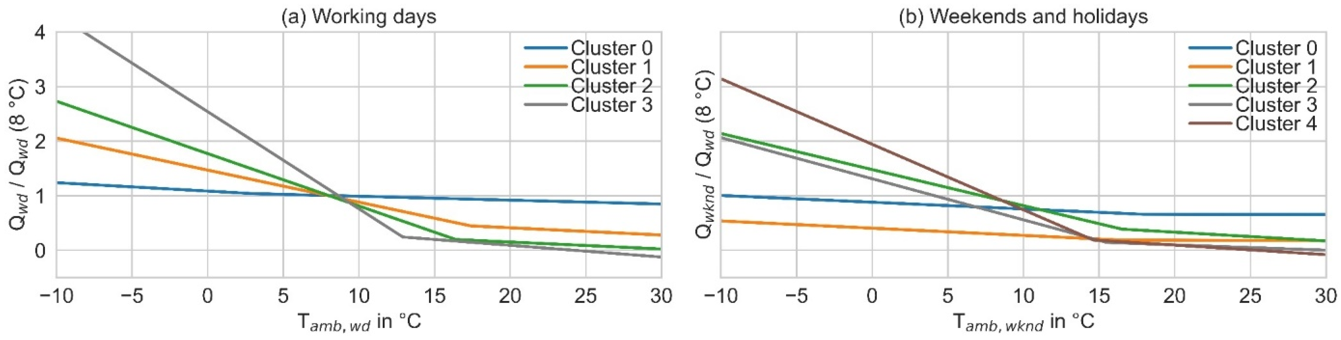
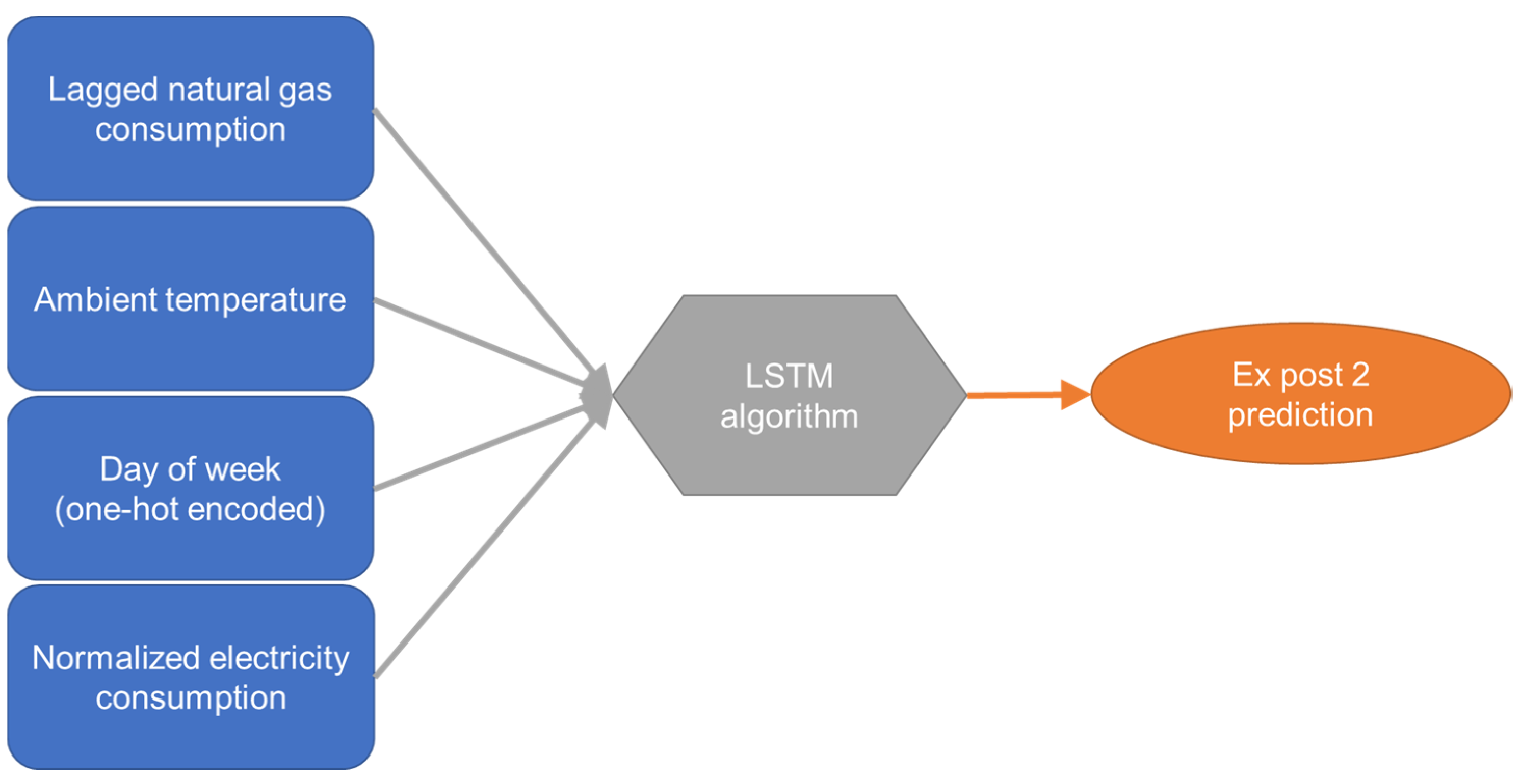
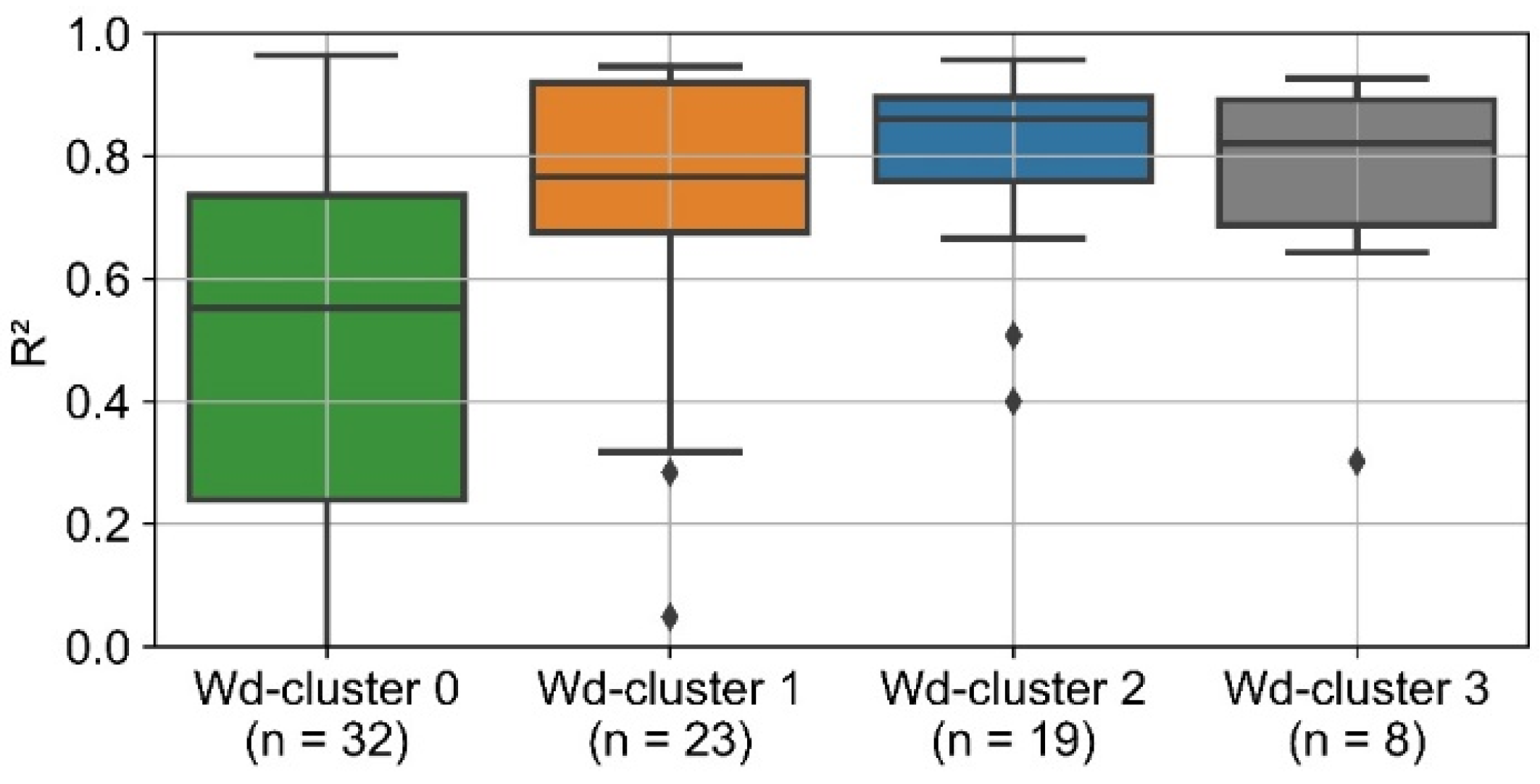
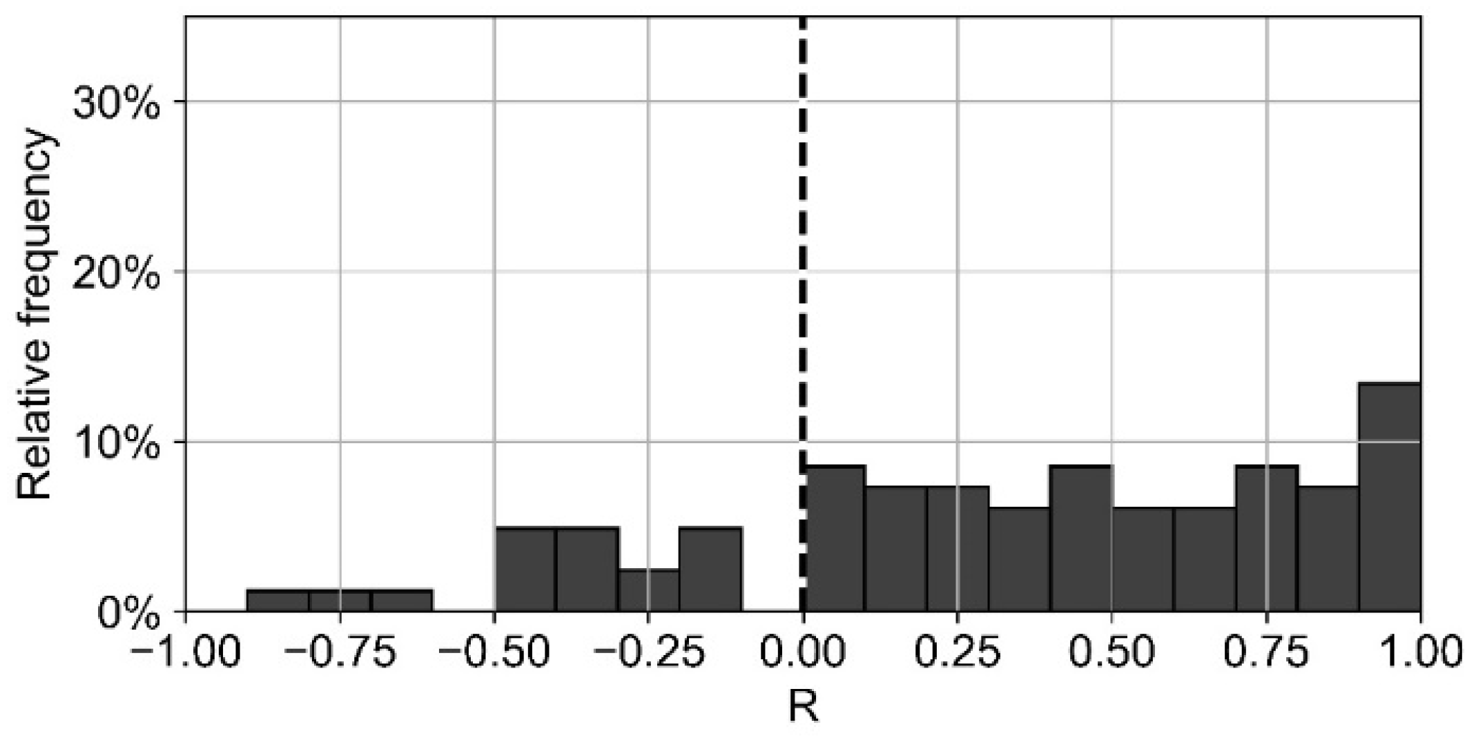
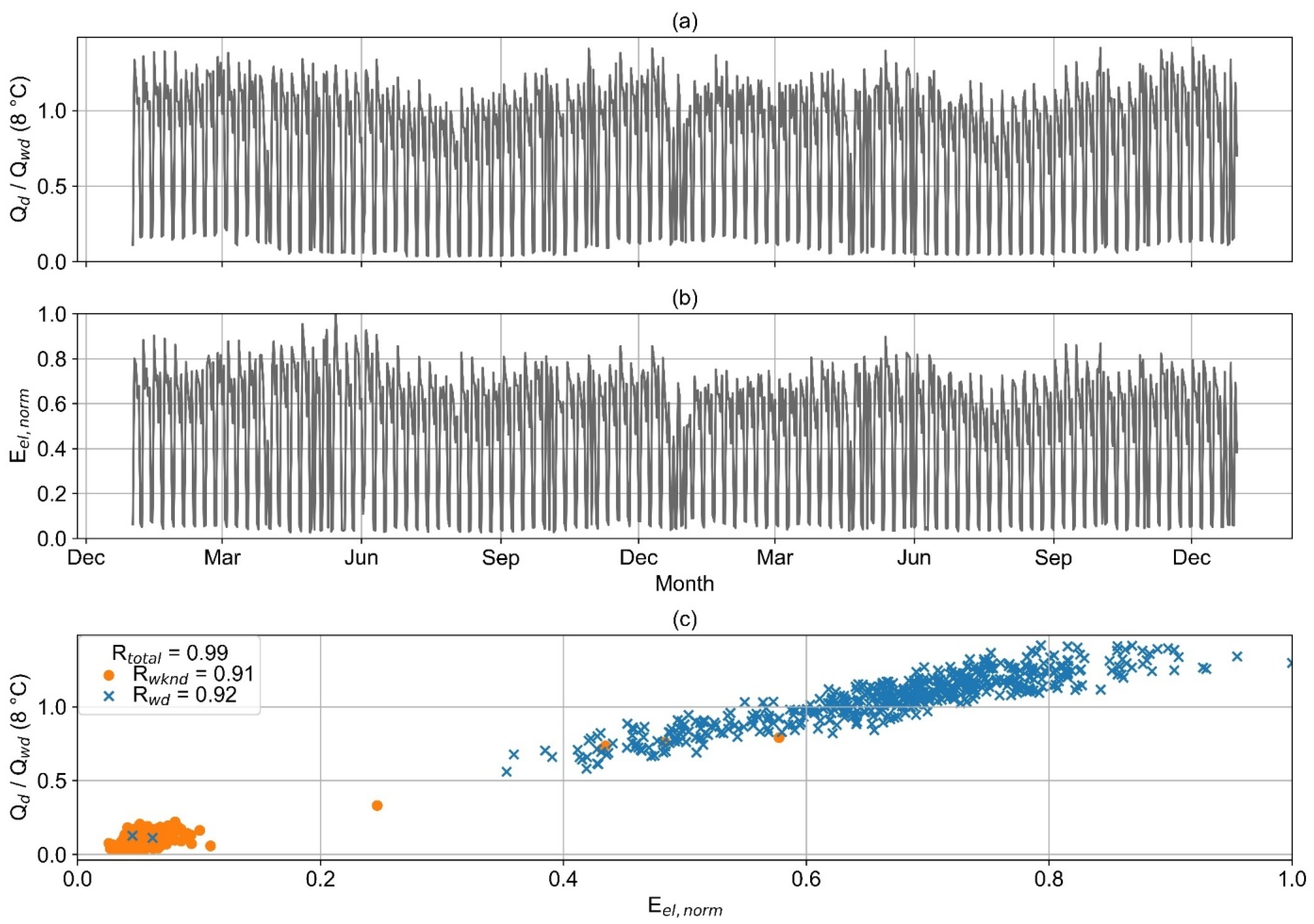
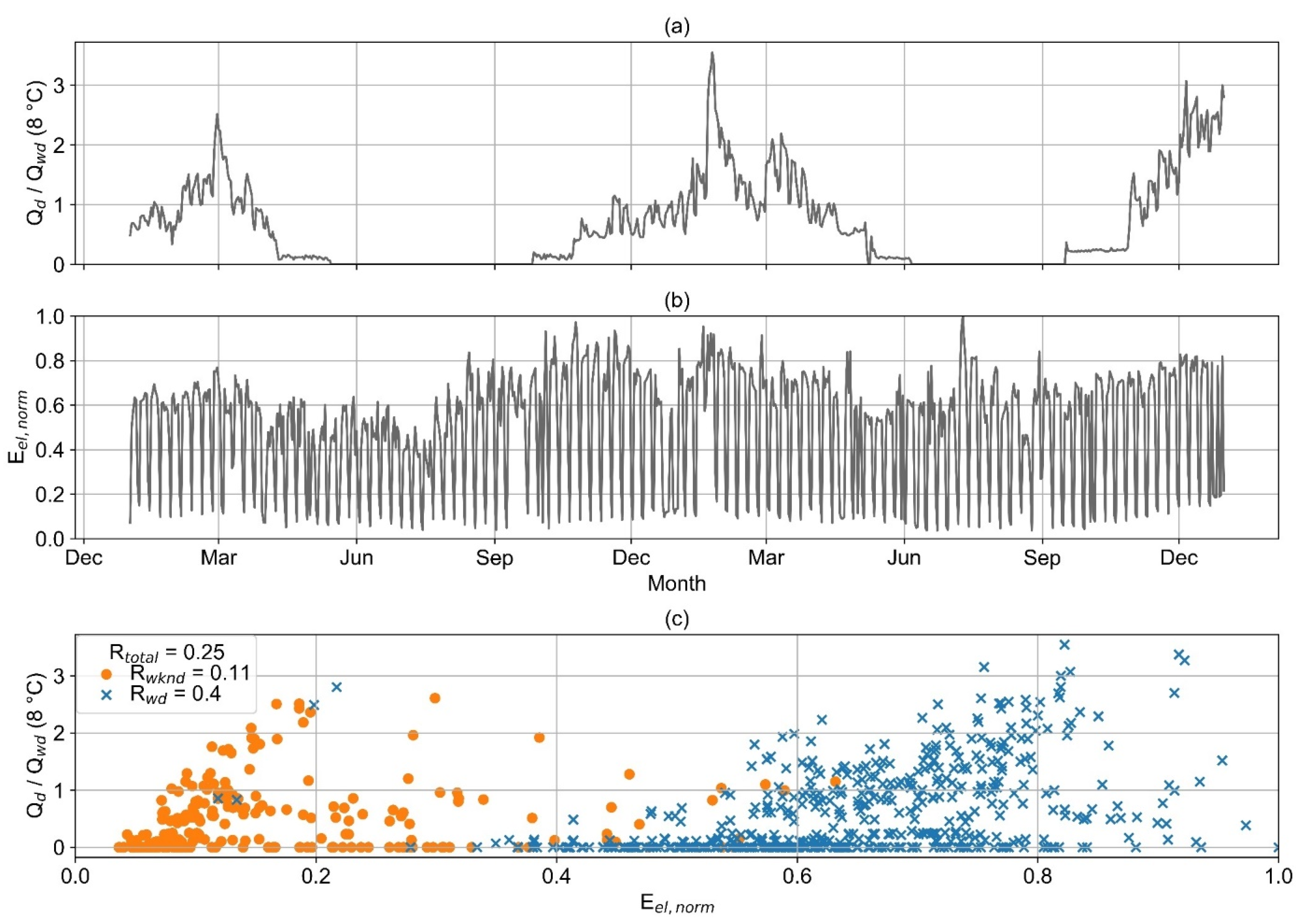
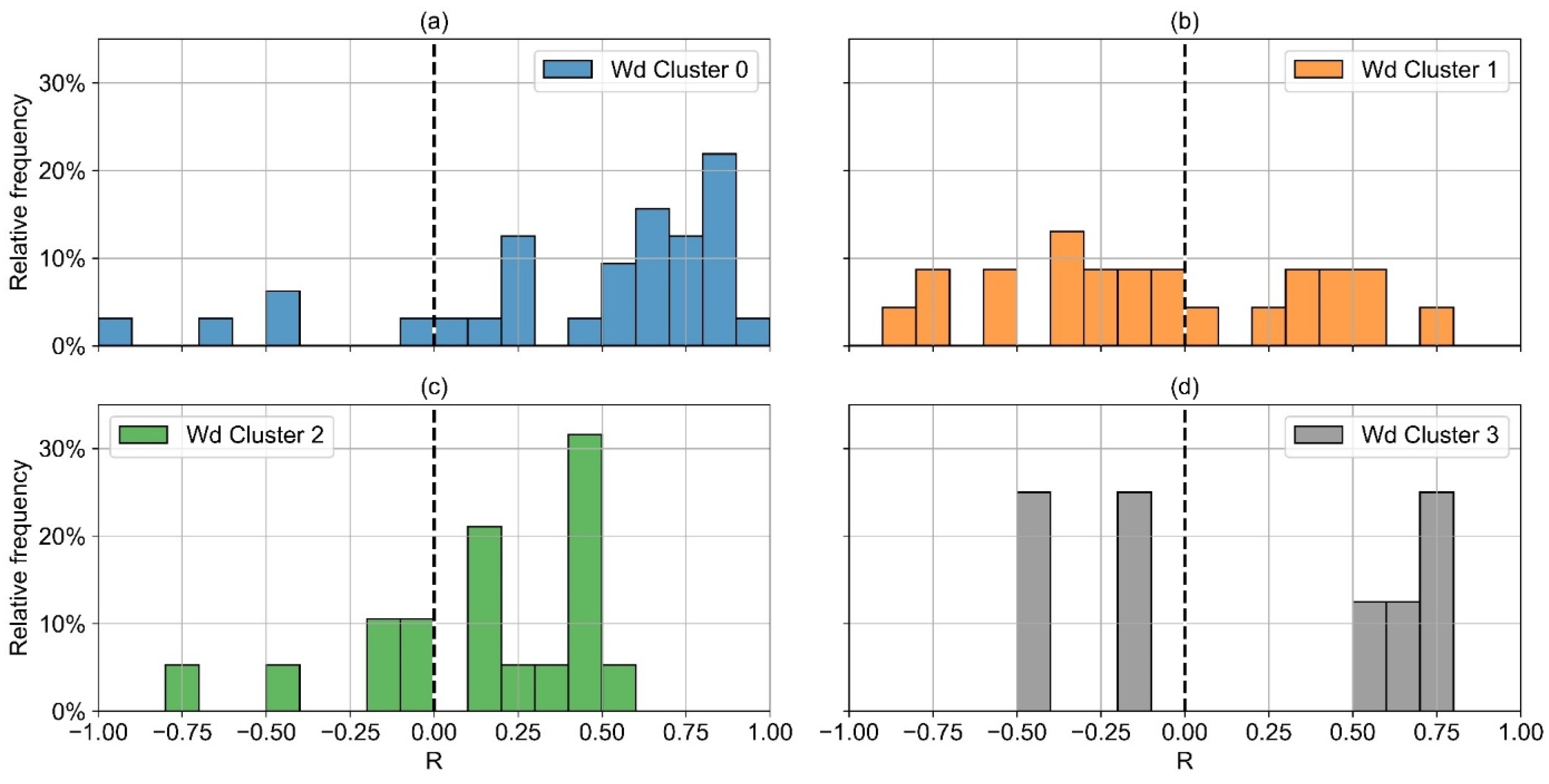
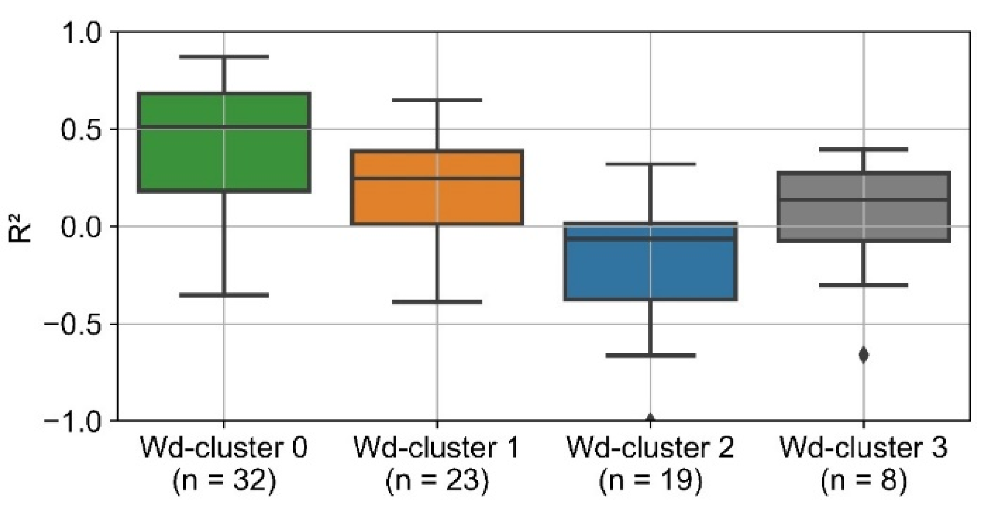
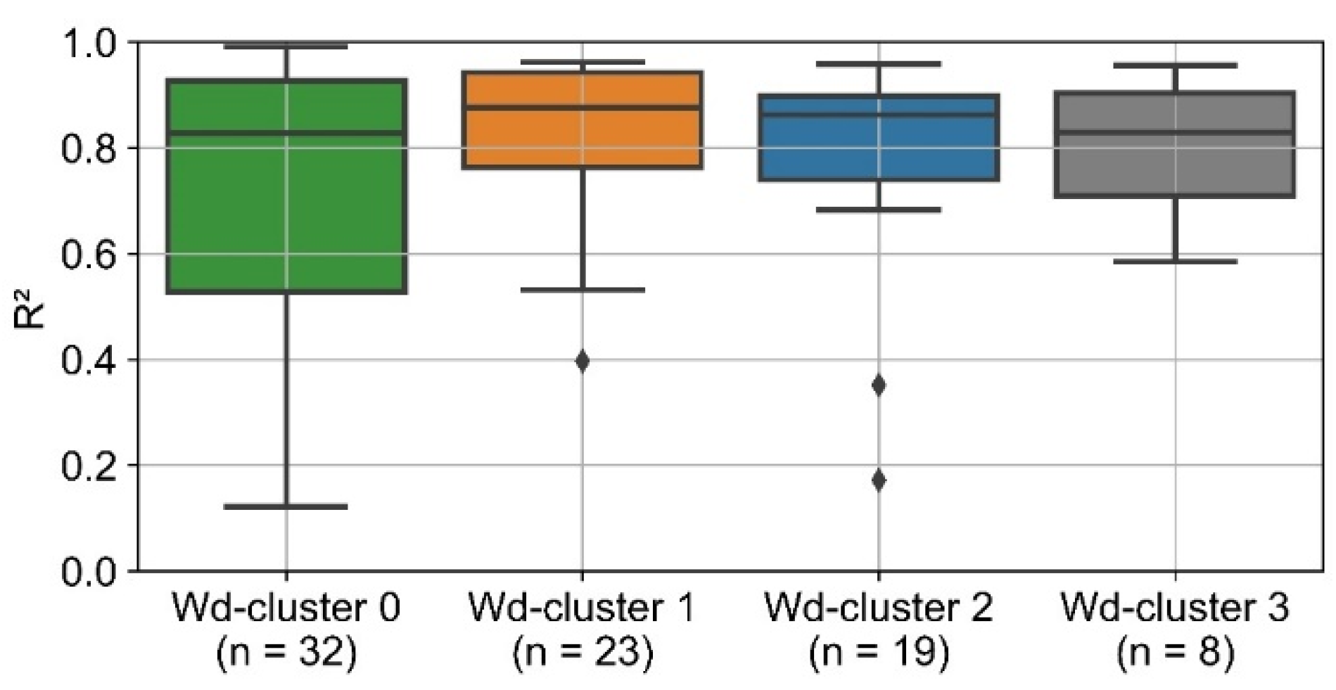
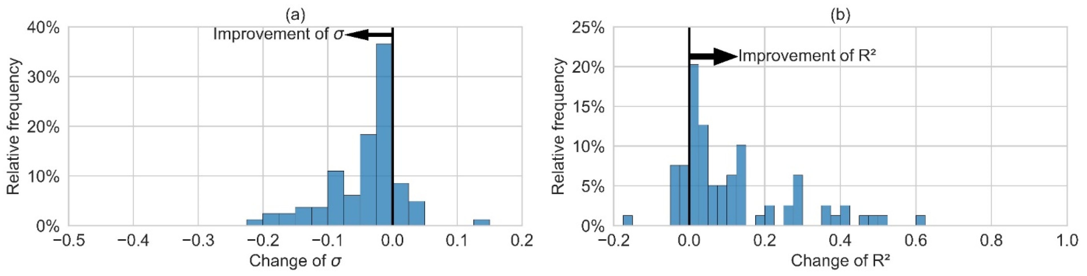
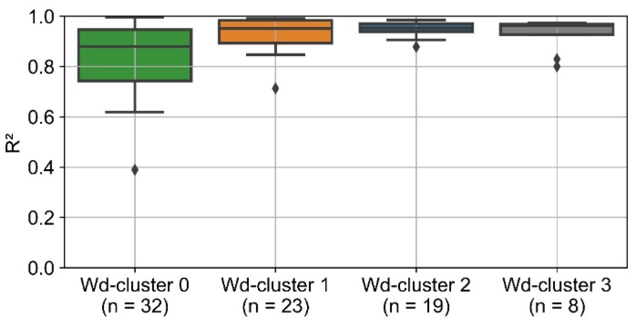
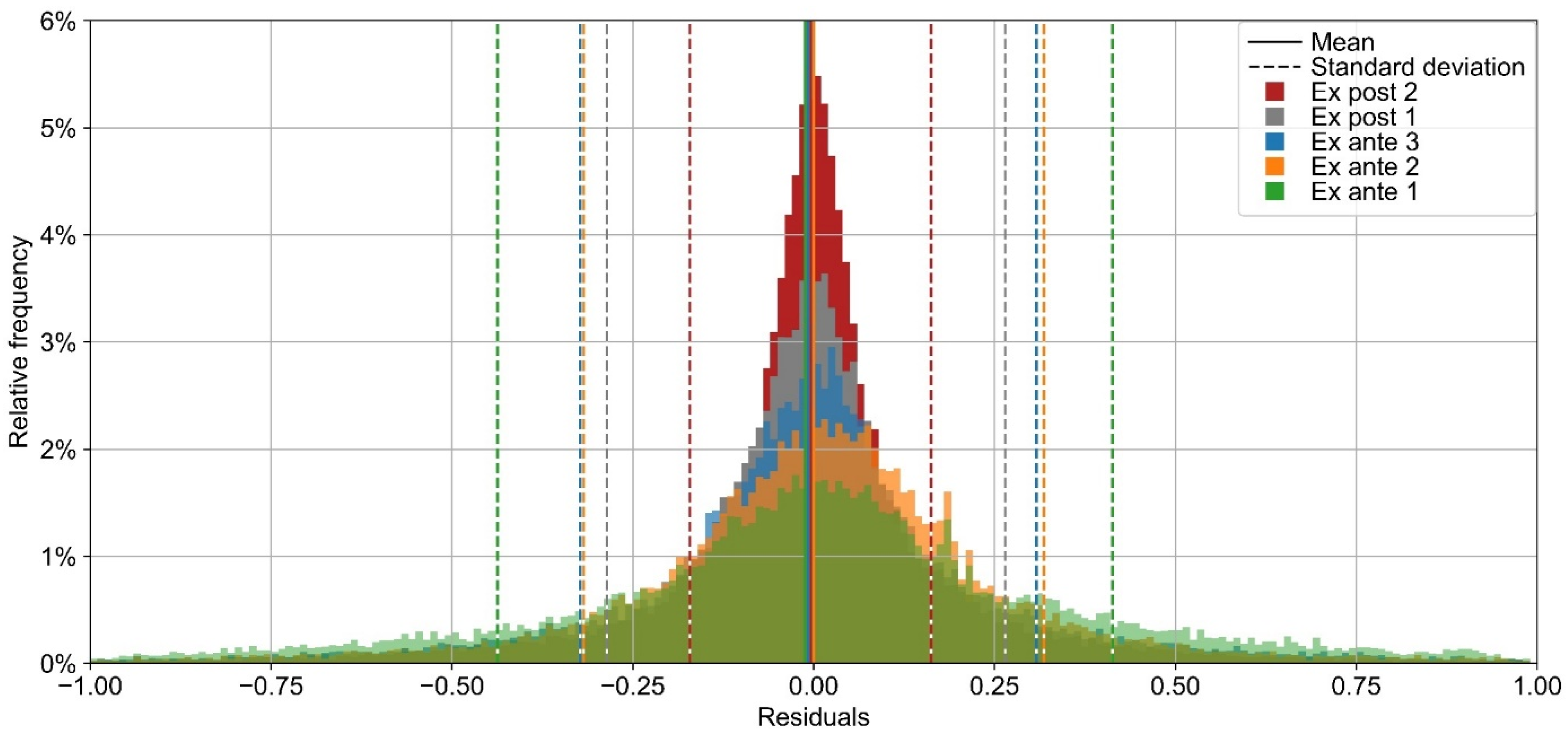
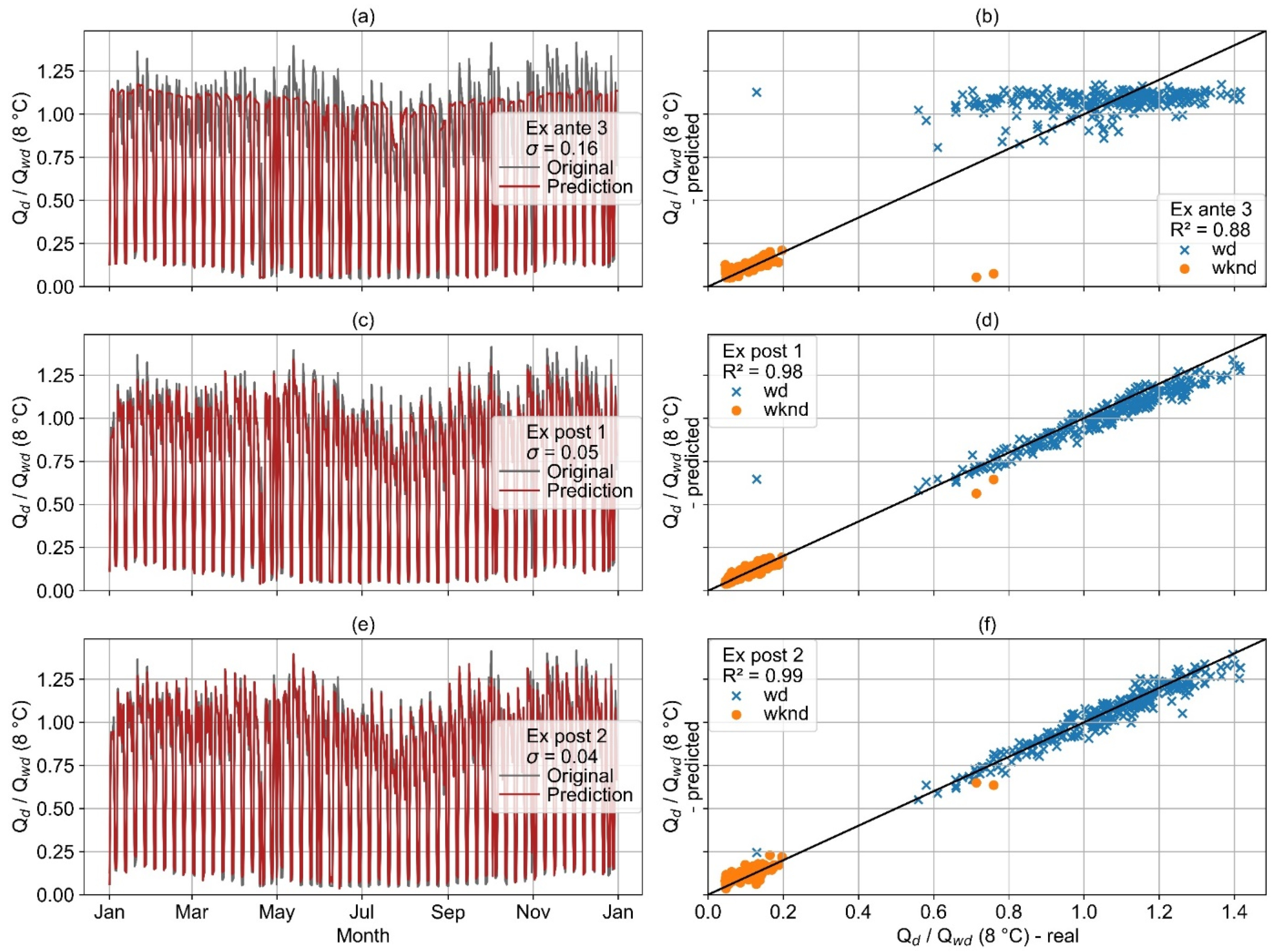
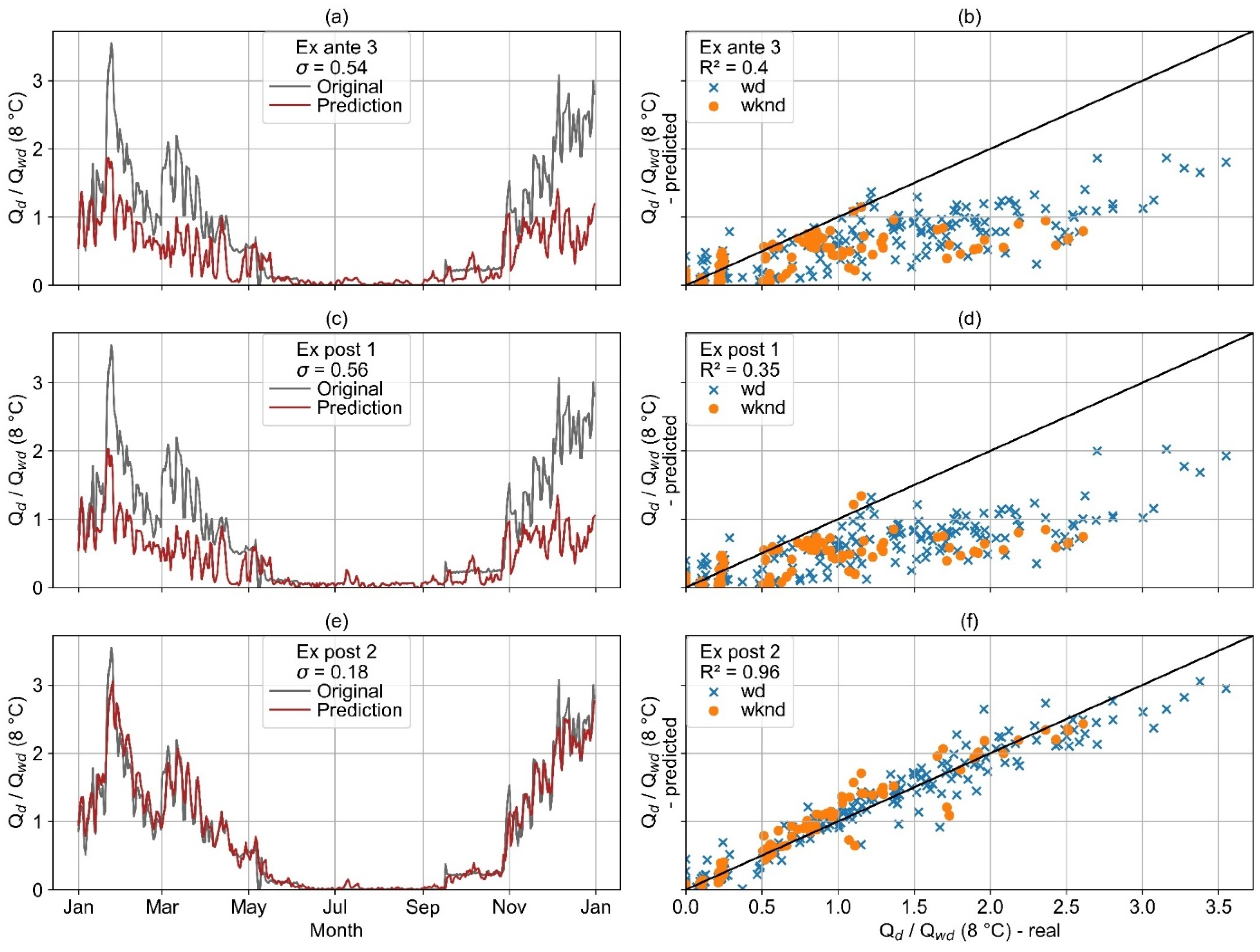