Article

Contribution of the Order Ericales to Improving Paleoclimate Reconstructions

1
College of Science, Northwest A&F University, Xianyang 712100, China
2
Center for Ecological Forecasting and Global Change, College of Forestry, Northwest A&F University, Xianyang 712100, China
3
Department of Biology Sciences, Institute of Environment Sciences, University of Quebec at Montreal, C.P. 8888, Succ. Centre-Ville, Montreal, QC H3C 3P8, Canada
*
Author to whom correspondence should be addressed.
Sustainability 2022, 14(7), 4008; https://doi.org/10.3390/su14074008
Submission received: 14 February 2022 / Revised: 20 March 2022 / Accepted: 24 March 2022 / Published: 29 March 2022
(This article belongs to the Section Air, Climate Change and Sustainability)

Abstract

:
Paleobotanists have long built leaf climate models based on site mean of leaf physiognomic characteristics of woody dicotyledons species (WDS) for estimating past climate. To explore the potential of the order Ericales in estimating paleoclimate, we developed two linear models for each climatic factor. One is based on WDS, and the other is based on both WDS and leaf physiognomic characters of the order Ericales (WDS-E). We found that, compared with WDS models, WDS-E models improved greatly in mean annual precipitation (MAP), growing season precipitation (GSP) and mean annual range in temperature (MART). When the minimum species number of the order Ericales is three per site, the WDS-E models improved the r2 from 0.64 to 0.78 for MART, from 0.23 to 0.61 for ln(MAP), and from 0.37 to 0.64 for ln(GSP) compared with the WDS models. For mean annual temperature (MAT), the WDS-E model (r2 = 0.86) also exhibited a moderate improvement in precision over the WDS model (r2 = 0.82). This study demonstrates that other patterns, such as those of the order Ericales, can contribute additional information towards building more precise paleoclimate models.

1. Introduction

With global warming and the frequent occurrence of extreme weather events (such as drought), climate change is becoming the main threat to the future of sustainable development of human beings [1]. Accurate paleoclimate estimation can help scientists to study and understand how environmental factors, such as greenhouse gases in the atmosphere, affect the Earth’s climate over time. Then, they can develop models to help predict how the increase of greenhouse gases and other changes may affect the future global climate [2]. This will help governments to formulate sustainable development measures.
Leaf physiognomy (size and shape) is strongly correlated with mean annual temperature (MAT) [3,4,5,6,7,8,9,10] and mean annual precipitation (MAP) [11,12,13,14,15,16,17]. Based on these relationships, a variety of leaf physiognomic methods have been developed for reconstructing paleoclimate, including the famous univariate methods, leaf-margin analysis (LMA) [6,13] and leaf-area analysis (LAA) [18,19], and multivariate methods, Climate-Leaf Analysis Multivariate Program (CLAMP) [14,20] and digital leaf physiognomy (DLP) [8,21]. The LMA and LAA are used for estimating MAT and MAP, each based on a single variable, the percentage of untoothed species at a site and site-mean leaf size, respectively. In order to improve the accuracy of univariate methods, Wolfe [14,20] developed CLAMP, which could estimate 11 leaf climatic factors by using 31 classified leaf states. This method has been widely used and most thoroughly tested [22,23,24]. At present, the whole CLAMP database contains 424 modern vegetation sites from all over the world [24]. The DLP is also a multivariable method, mainly using continuous variables, which can be used to estimate 10 climatic factors [23], including the growing season precipitation (GSP) and mean annual range in temperature (MART). The DLP method has been tested several times, and it has shown its potential in paleoclimate estimation [10,25]. In the current DLP dataset, there are 92 natural or naturalized vegetation sites.
Current leaf-physiognomy climate models using these methods are site-based: that is, climate is estimated from the site mean of leaf physiognomic characteristics of woody dicotyledons species (WDS) [26]. Such estimations require an assumption, to some extent, that leaf physiognomy responds to climate in the same way, regardless of the species [27,28,29]. The results of some studies did not support this hypothesis. Royer et al. [30] found that there were many significant correlations between MAT and leaf physiognomic variables in Acer rubrum, such as the number of teeth (#Teeth; r2 = 0.54, p < 0.0001) and blade area (r2 = 0.38, p < 0.0001), but in Quercus kelloggii, these correlations were weaker. An experiment about the effects of leaf physiognomy on temperature in five species also supported the view that the temperature effects on leaf shape are usually species-specific, so leaf-climate models should take into account species-specific responses [26]. Studies [10,31] also showed that there were significant differences between individual climate and tooth size, shape, and number, Feret’s diameter ratio and leaf size within evergreen than in deciduous species among woody taxa at individual sites. This also means that other patterns, not only the across-species mean of leaf physiognomy, may contribute useful information for estimating paleoclimate. Therefore, constructing leaf climate models using only the variables of WDS may mask different responses of different species, different families, and different orders to climate. This is not conducive to the construction of precise models. It is necessary to test whether independent variables of leaf physiognomy in other patterns, such as within the order Ericales or the order Rosales, could provide useful information for paleoclimate estimation. To the best of our knowledge, very few studies have tested the potential use of the order Ericales for improving leaf-climate models.
Ericales is a large and diverse dicotyledonous plant order that includes about 1200 species in 21 or 22 families, with its members distributed all over the world [32,33]. Some families are almost cosmopolitan. For example, Ericaceae, as the dominant group of plants, is distributed in vast areas of the northern hemisphere, forming a unique heather ecosystem. Some families are pan-tropical (e.g., Ebenaceae, Lecythidaceae and Sapotaceae), while others are restricted to neotropics (e.g., Marcgraviaceae and Theophrastaceae) or concentrated in more temperate regions (e.g., Clethraceae, Cyrillaceae and Primulaceae) [34]. Ericales is also one of the orders with the largest sample size in the DLP raw dataset. However, the relationship between leaf physiognomy of the order Ericales and climate is still poorly known. This limits our general understanding of the relationships between leaves and climate, and also limits the value of the order Ericales in paleoclimate reconstructions.
The purpose of this study is not to refute the outstanding performance of previous methods of leaf climate in reconstructing paleoclimate, such as the CLAMP and the DLP, in which leaf physiognomic datasets are built by WDS, but rather to explore the potential use of physiognomic variables for the order Ericales as climate proxies. This study will test: (1) the correlation between leaf physiognomy of the order Ericales and climate; (2) whether independent physiognomic variables of the order Ericales can contribute useful information for establishing more precise models, compared with models built only by independent physiognomic variables of WDS; and (3) whether the accuracy of linear models has great difference with the change of species richness of the order Ericales within sites.

2. Materials and Methods
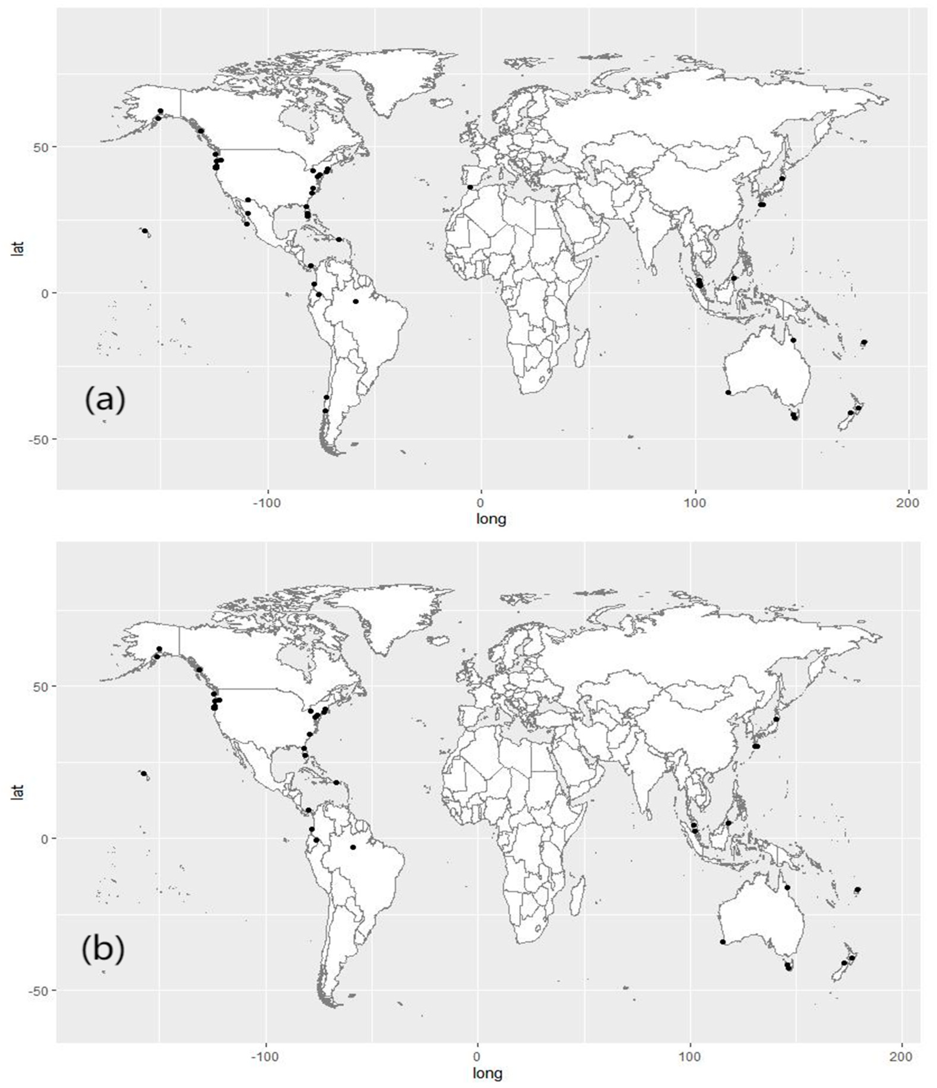
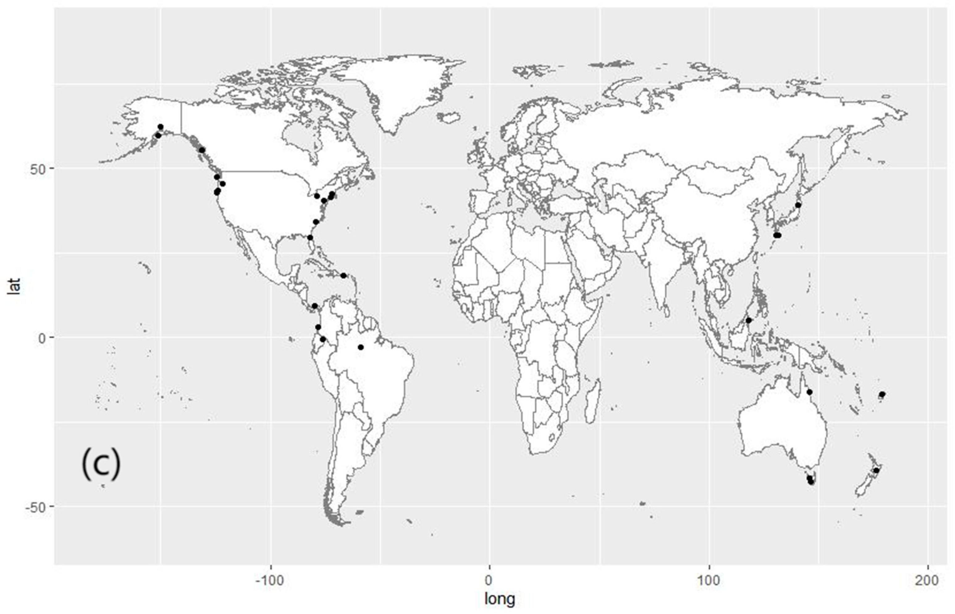
2.1. Dataset

Although the CLAMP global dataset has more modern vegetation sites than that of the DLP dataset, the CLAMP method mostly uses canonical correspondence analysis to infer climate, while the DLP method mostly uses linear models. In this study, we will mainly use linear models for research. Therefore, we chose the DLP method for analysis. The dataset of the order Ericales was calculated from the raw DLP dataset [10]. The definitions of leaf physiognomic characters were based on the research of Royer et al. [8]. Using these characteristics of leaves, we constructed a total of 27 variables. In the DLP dataset, we first selected the sites with at least two species of the order Ericales. For the order Ericales, species means were first calculated, then site means of the order Ericales were derived from the species means. In the dataset of the order Ericales, there are 55 modern vegetation sites, and each site has at least 2 Ericales species (Figure 1a), 44 modern vegetation sites, each with at least 3 species of the order Ericales (Figure 1b) and 32 modern vegetation sites, each of which has at least 4 species of the order Ericales. (Figure 1c). In order to distinguish the variables in the different datasets, we prefixed the variable names in the order Ericales with E.
Climate data were extracted from a global, interpolated 1-km spatial resolution climate model (WORLDCLIM) [35]. The MAT of the order Ericales sites ranged from 0.8 to 27.7 °C, the MART ranged from 0.8 to 27.0 °C, the MAP ranged from 19 to 680 cm, and the GSP ranged from 15 to 469 cm. The Supplementary Materials provide definitions and data of all leaf physiognomic and climate variables used in this study (Supplementary Tables S1 and S2).

2.2. Correlation Analysis

Pearson correlation analysis is the most commonly used method to measure the strength of the linear relationship between two numerical variables [36]. It assigns a value between −1 and 1 called the Pearson correlation coefficient, where 1 is a total positive correlation, −1 is a total negative correlation, and 0 indicates that there is no linear relationship between the two variables. As in previous research [10,30], this method was used to quantify the relationship between leaf characteristic variables and climate variables, and statistically significant correlations is measured by p-value (p < 0.05).

2.3. Method of Establishing Linear Models

Although there is a complex relationship between plant leaf characters and climate, the nonlinear leaf climate models also show better performance than linear models [23,25], we still choose building linear leaf climate models to explore the potential of the order Ericales. For one reason, it is more complicated and difficult to establish an optimal or relatively optimal nonlinear model than a linear model. For another reason, the main tool of the applied statistician remains the linear model [37].

2.3.1. Variable Selection Method for Establishing Multiple Linear Models

We select variables of the linear models in two steps. The first step is accomplished by stepwise regression. Subset regression is helpful to establish the optimal linear model, but when there are too many candidate independent variables, this is very difficult [38]. By contrast, stepwise regression is a simple and practical method. Although it can only construct a relatively optimal model in many cases, it is commonly used in variable selection and is often reported in empirically-based journal articles [39]. In our datasets, there are at least 27 candidate independent variables for building models. Therefore, we used stepwise regression to establish linear models. In this step, two criteria were used: (1) all independent variables were required to be significant at the p = 0.05 level; (2) all independent variables did not show a high degree of collinearity with the other predictor variables (variance inflation factor) [40]. This work was conducted in SPSS 21 [41]. When the first step was completed, we then tried to delete some unnecessary variables to improve the model precision and avoid over-fitting. The criteria of whether a variable was deleted from the model is based on the r2 of 10-fold cross-validation. If the r2 of the model did not decrease when a variable was deleted, then we would remove it from the model; otherwise, we would retain it.

2.3.2. Robust Regression

In regression analysis, the ordinary least square method is commonly used to estimate the parameters of linear models. However, this method is sensitive to outliers, and it needs the data to meet the assumption that the error distribution is normal, otherwise it will behave poorly. Robust regression is a method of robust estimation in statistical regression analysis which can solve the problem. “Modern Applied Statistics with S (MASS)” introduces the theory of robust regression [42]. The main concept of robust regression is to eliminate or weaken the influence of outliers on parameter estimation by iteratively weighting the objective function of ordinary least square regression so as to ensure the reliability of results. The most common method of robust regression is M- estimation [43] which can be regarded as a generalization of maximum-likelihood estimation. In R software of version 3.4.1, the rlm() function in the “MASS” package could be used to realize M-estimation.

2.4. Evaluation of Model Precision

2.4.1. 10-Fold Cross-Validation

K-fold cross-validation is a widely used statistical method for estimating the predictive ability of models. In k-fold cross-validation, firstly, the dataset is divided into k equal (or approximately equal) sub-datasets. One dataset is used for validation, while the other k-1 datasets are used for model training. This process is repeated k times until the entire dataset is used for validation. Finally, the evaluation index of the model on k different sub-datasets are averaged to get the overall evaluation index of the model. However, the estimated value fluctuates under the influence of random sampling. In order to provide a reliable estimate, a common strategy is to perform 10 times of 10-fold cross validations [44]. Here, the repeated cross-validation indexes of the models (i.e., RMSE and r2) was calculated in R version 3.4.1 [45].

2.4.2. Stratified Random Sampling in Cross-Validation

Stratified random sampling is a probability sampling method and a form of random sampling in which the population is divided into two or more groups (strata) according to one or more common attributes. It can ensure that the proportion of each category is approximately equal to the proportion of the population data after random division [46]. In 10-fold cross-validation, we used stratified random sampling to divide the sub-datasets.

2.4.3. Evaluation Indexes of Linear Models

The determination coefficient (r2) and Root Mean Squared Error (RMSE) are mainly used as evaluation indexes of models, and we used them to evaluate the precision of each model here. The definitions of r2 and RMSE are as follows:
r 2 = 1 i = 1 n ( y i y ^ i ) 2 i = 1 n ( y i y i ¯ ) 2
RMSE = 1 n i = 1 n ( y i y ^ i ) 2
where n is the number of observations or samples, y i is the observed value, y ^ i is the predicted or estimated values, and y i ¯ is the average of the observed values.
The index r2 measures the portion of the observation change that is explained by the predictions, and is usually between 0 and 1. However, r2 can also be less than 0 when it is calculated in cross-validation. The closer r2 gets to 1, the closer the prediction is to the observation. RMSE measures the average deviation between the predicted and the observed values. The smaller the RMSE value, the closer the prediction is to the observation. In order to evaluate the potential of the independent variables of the order Ericales in past climate estimation, two-class multivariate linear models were established. One was established based on the leaf physiognomic variables of WDS, while the other was established based on leaf physiognomic variables of both WDS and the order Ericales (WDS-E).

3. Results

We first built leaf-climate linear models by the stepwise regression method based on the dataset which contained at least three species per site, and found that physiognomic variables of the order Ericales were of great help to improve the fitting precision of MAT, MART, MAP, and GSP. Therefore, here we only present the correlation analysis between the order Ericales and these four climate factors, and establish two class models for these four climatic factors.

3.1. Correlations between Physiognomic Variables of the Order Ericales and Climatic Variables

Many leaf physiognomic variables of the order Ericales are significantly correlated with MAT (Supplementary Table S3). Notably, there is a significant positive correlation between MAT and many leaf size-related variables, including E-ln (leaf area) (r2 = 0.48, p < 0.001), E-Feret’s diameter (r2 = 0.38, p < 0.001), E-Perimeter (r2 = 0.37, p < 0.001), E-Major length (r2 = 0.37, p < 0.001), and E-ln (internal perimeter) (r2 = 0.37, p < 0.001). Among these variables, E-ln (leaf area) has the strongest correlation with MAT, while among the leaf physiognomic variables of WDS, percent of untoothed species has the strongest correlation with MAT [10]. In addition, MAT shows a negative correlation with E-Primary teeth (r2 = 0.10, p < 0.05), E-#Teeth (r2 = 0.10, p < 0.05), and some other teeth-related variables, such as E-#Teeth/Peri (r2 = 0.22, p < 0.001), E-#Teeth/IntPeri (r2 = 0.22, p < 0.001), E-#Teeth/BA (r2 = 0.27, p < 0.001) and TA/BA(r2 = 0.11, p < 0.05). These results suggest that the order Ericales in cold climates generally has fewer and smaller teeth.
There are significant negative correlations between MART and many leaf size-related variables, such as E-blade area(r2 = 0.19, p < 0.001), E-Leaf area (r2 = 0.19, p < 0.001), E-Perimeter (r2 = 0.26, p < 0.001), E-Feret’s diameter (r2 = 0.24, p < 0.001), E-ln (Major length) (r2 = 0.26, p < 0.001), and E-Internal perimeter (r2 = 0.27, p < 0.001). This means the greater the change in MART, the smaller the leaf size.
Only a few physiognomic variables of the order Ericales correlate significantly with ln(MAP). Ln(MAP) is positively correlated with E-Perimeter (r2 = 0.11, p < 0.05), E-Internal perimeter (r2 = 0.10, p < 0.05) and E-Major length (r2 = 0.11, p < 0.05). These variables also have similar significant correlation with E-ln(GSP). This means that in humid climates, the leaves of the order Ericales are larger.

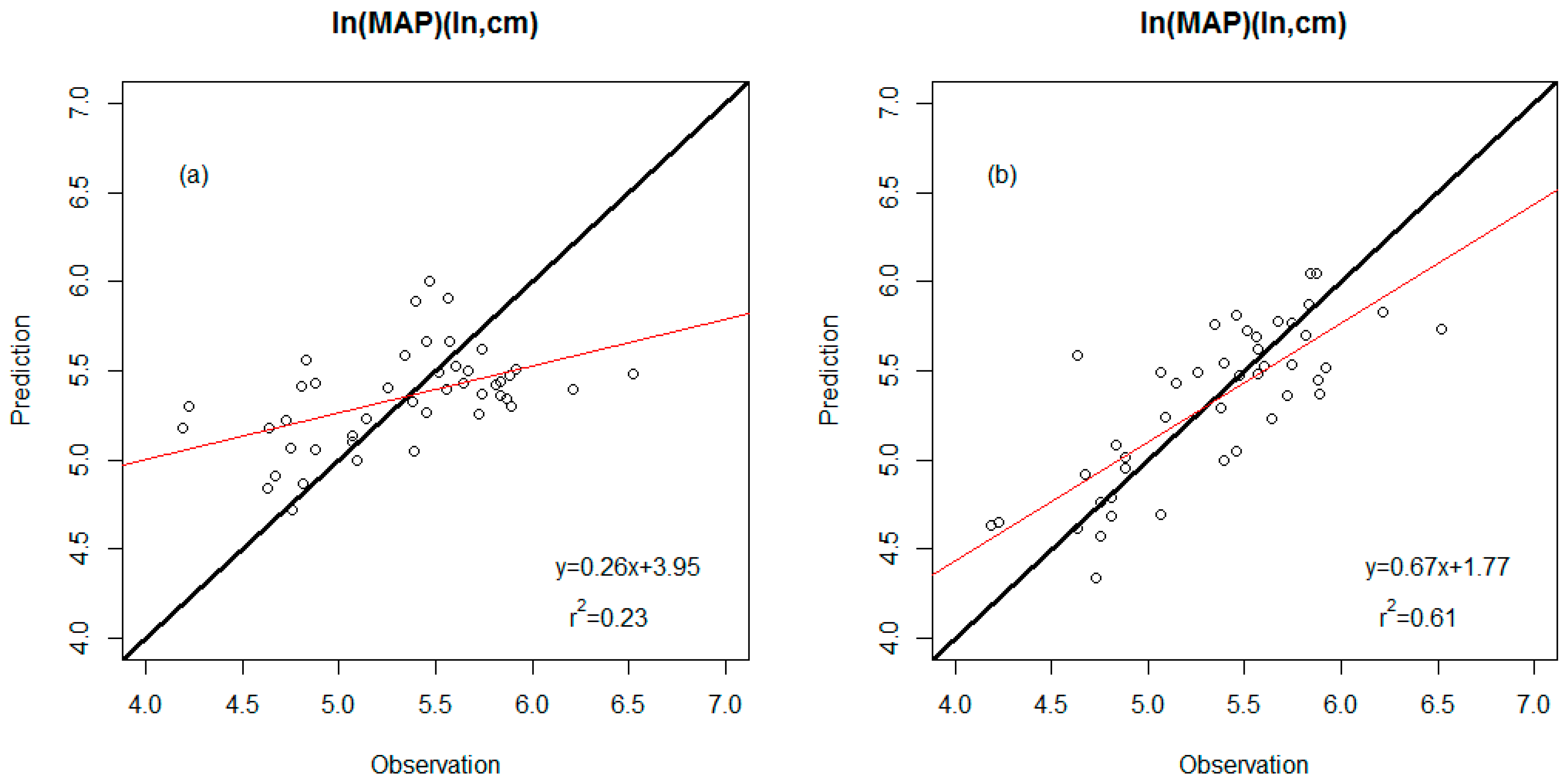
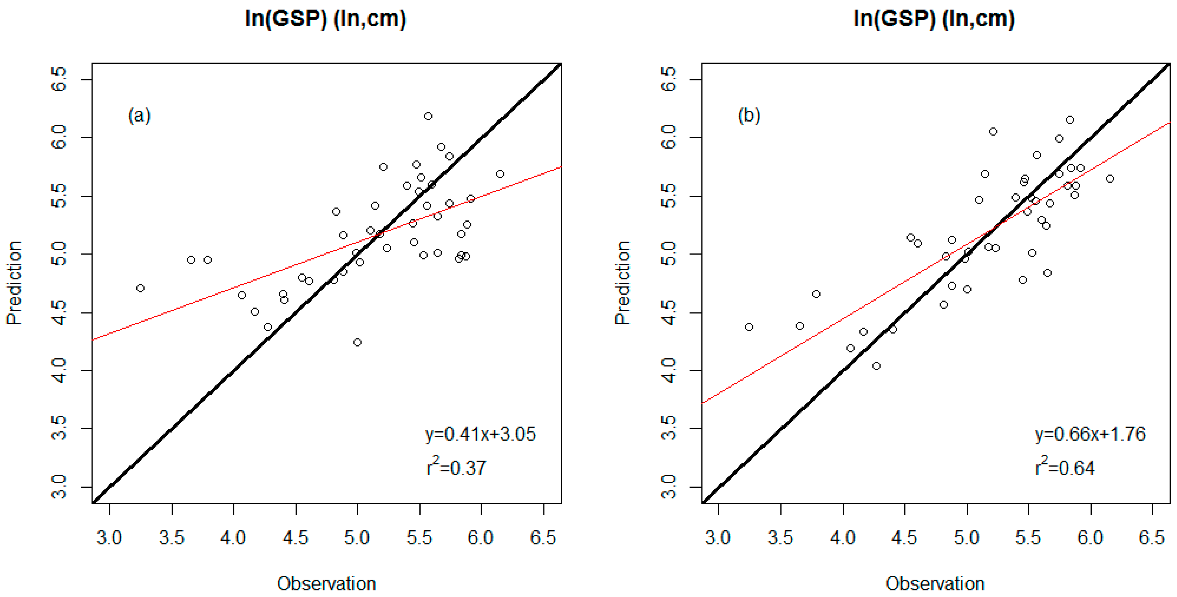
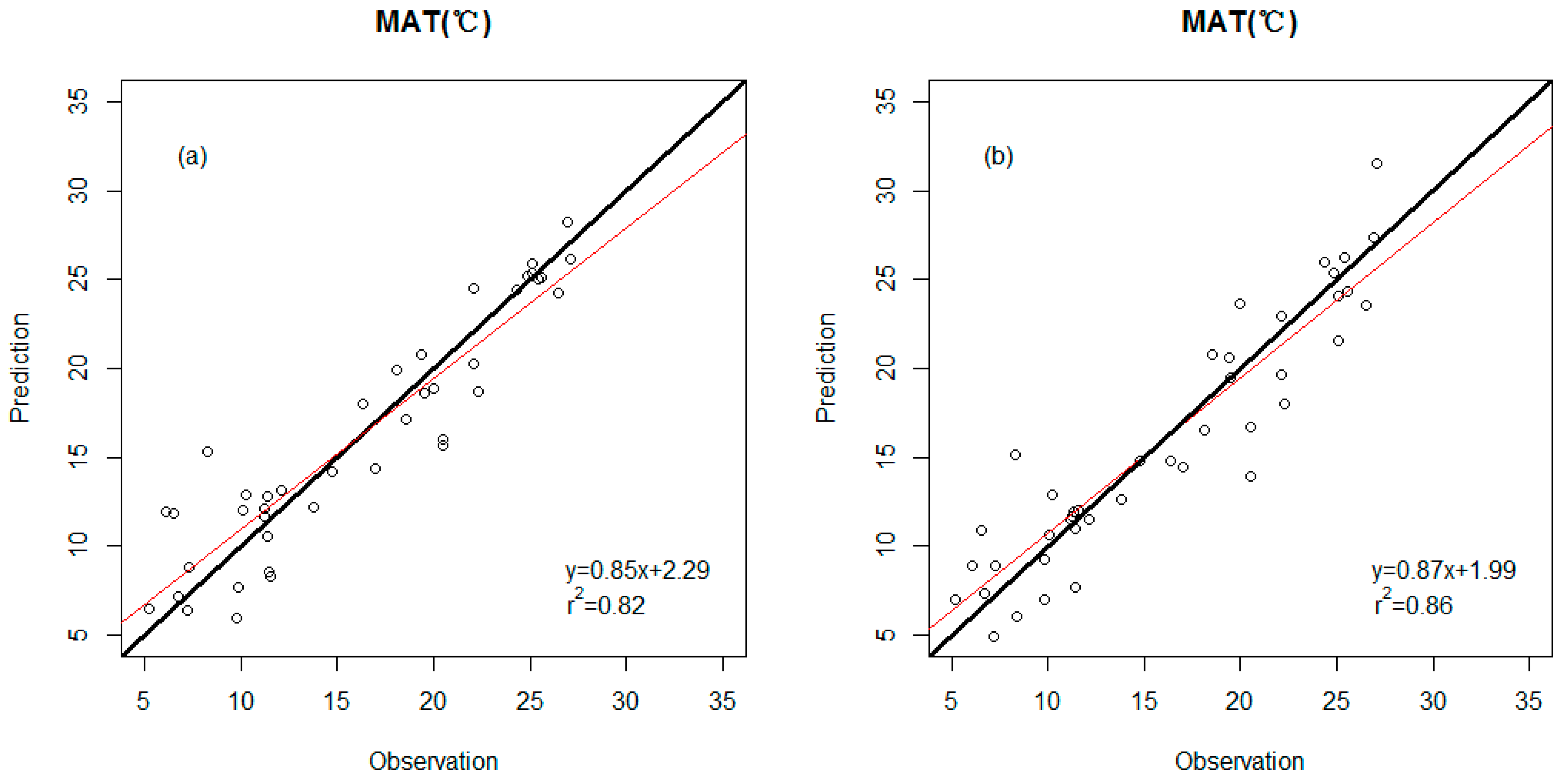
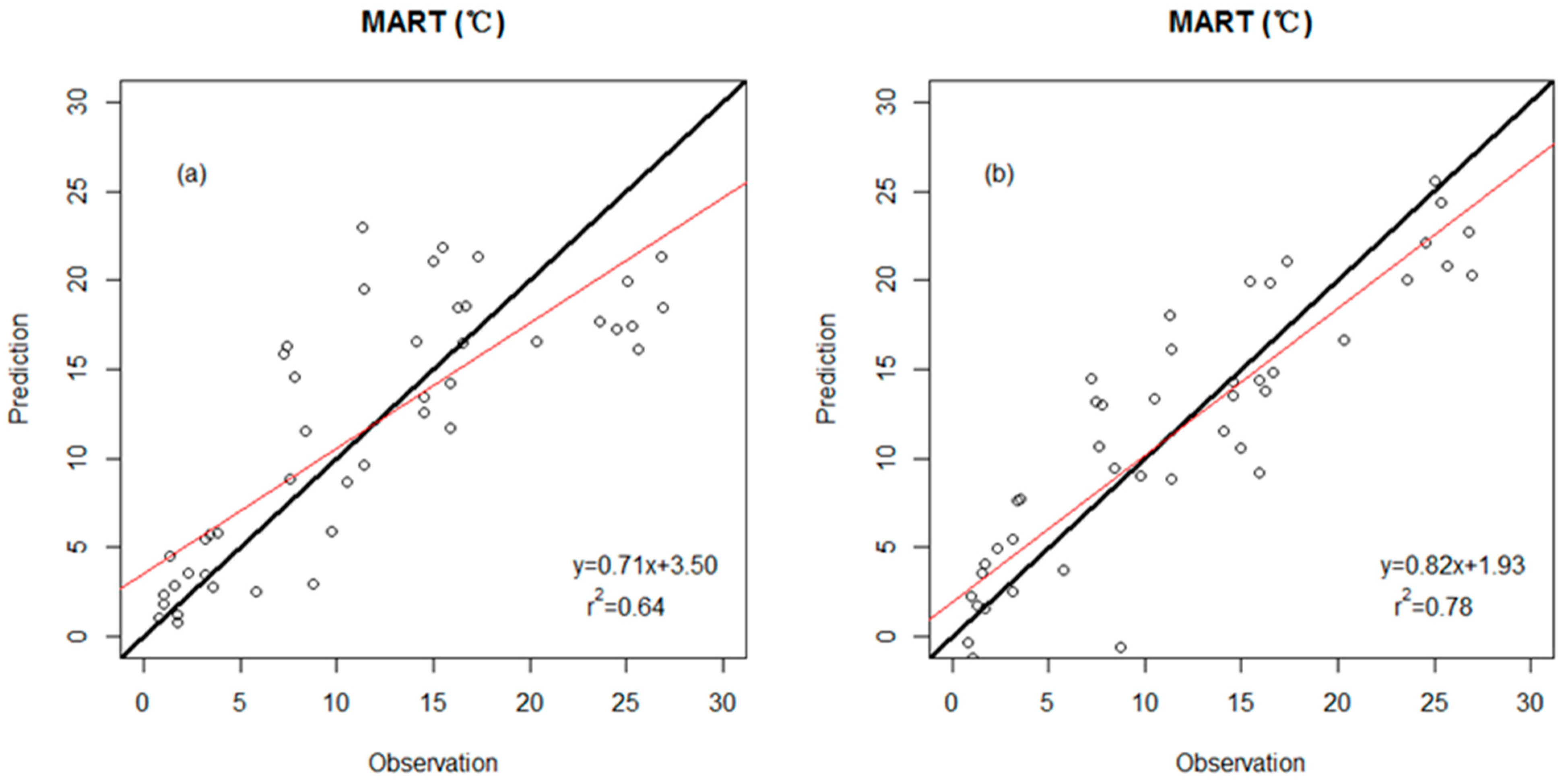
3.2. Precision Comparison of Two Classes of Linear Models

WDS-E and WDS models shown here are based on 44 modern sites which had at least 3 species of the order Ericales per site. Compared with the WDS models, the precision of all WDS-E models is improved (Table 1, Figure 2, Figure 3, Figure 4 and Figure 5). For MAT, the WDS-E linear model [RMSE = ±2.7 °C; r2 = 0.86; Table 1; Figure 2b] exhibits a moderate improvement compared with that of the WDS linear model [RMSE = ±3.1 °C; r2 = 0.82; Table 1; Figure 2a]. However, for MART, the precision of the WDS-E model [RMSE = ±3.8 °C; r2 = 0.78; Table 1; Figure 3b] is much higher than that of the WDS model [RMSE = ±4.9 °C; r2 = 0.64; Table 1; Figure 3a]. For ln(MAP), the WDS-E model has much better precision [RMSE = ±0.32 (ln, cm); r2 = 0.61; Table 1; Figure 4b] than the WDS model [RMSE = ±0.45 (ln, cm); r2 = 0.23; Table 1; Figure 4a]. For ln(GSP), the precision of the WDS-E model [RMSE = ±0.40(ln, cm); r2 = 0.64; Table 1; Figure 5b] also improves a lot compared with the WDS model (RMSE = ±0.53 (ln, cm); r2 = 0.37; Table 1; Figure 5a).

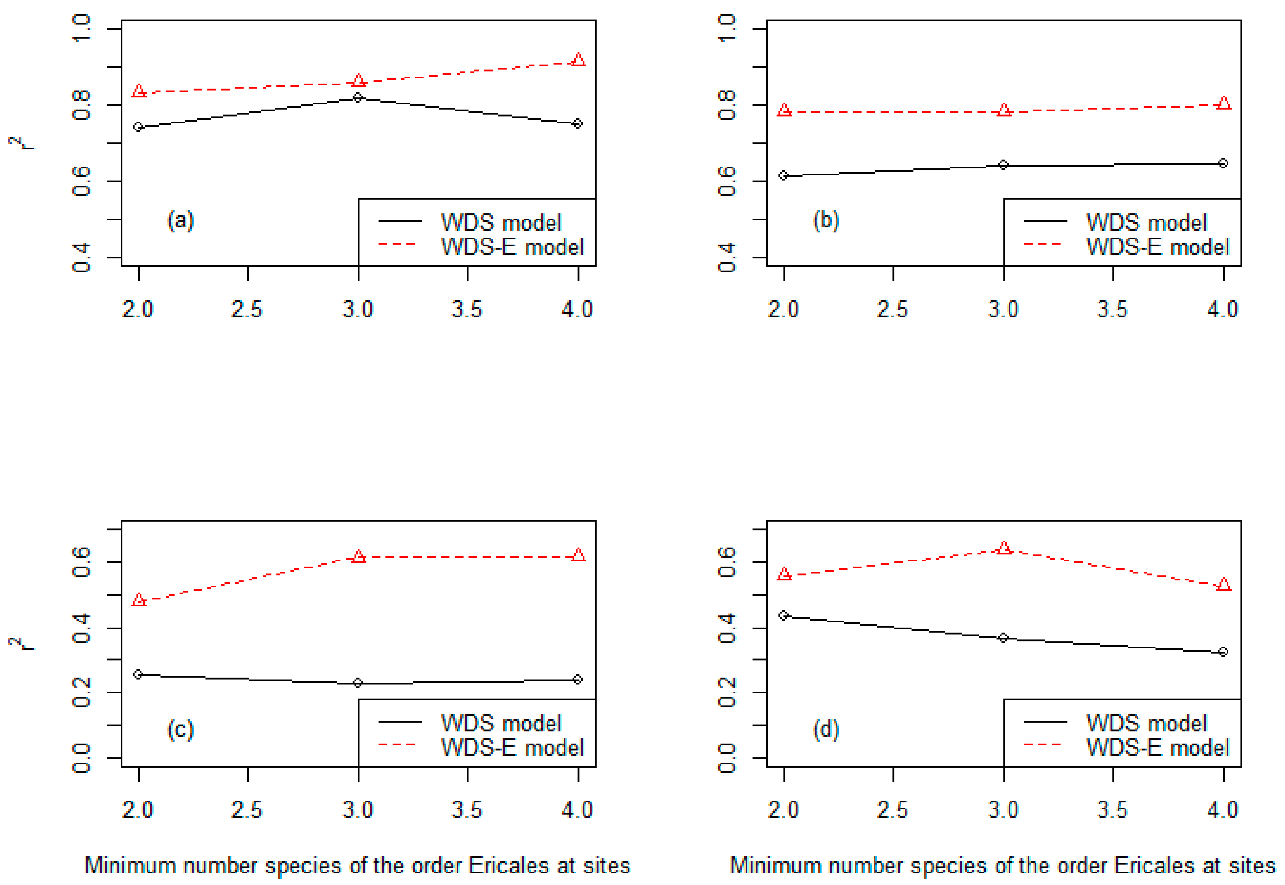
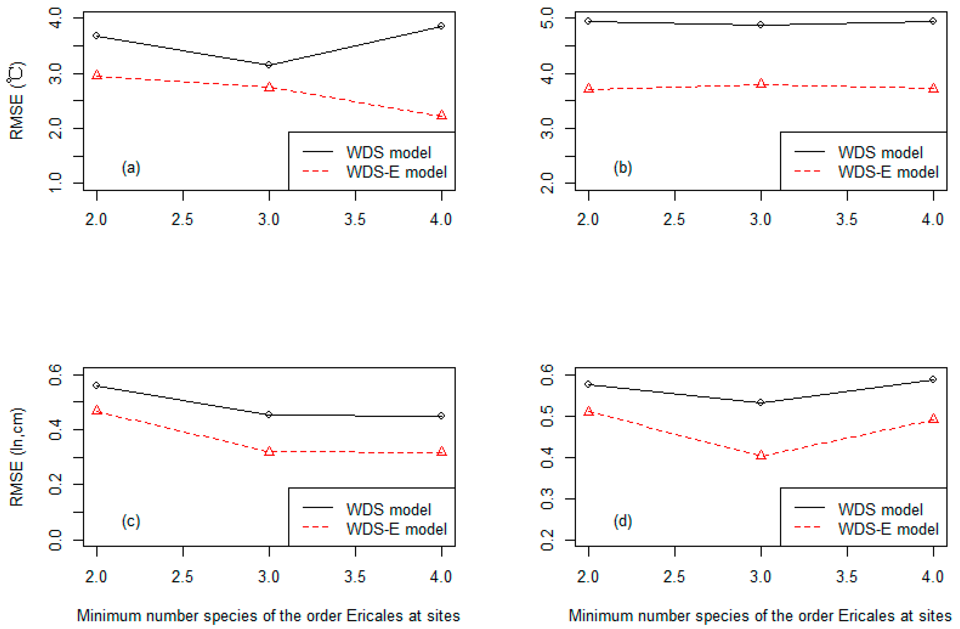
3.3. Precision of the Two Classes of Linear Models at Three Different Levels of the Species Numbers of the Order Ericales

To test whether the number of species of the order Ericales at sites affects the precision of the linear models, we also established linear models at the other two levels based on at least two species and on at least four species of the order Ericales per site, and calculated their prediction precision.
Based on the repeated 10-fold cross-validation, all WDS-E models have better prediction precision than corresponding WDS models, and their precision only fluctuates slightly at three different levels (Figure 6 and Figure 7). Compared with WDS models, WDS-E models have greatly improved for MART, MAP and GSP at all three levels. For MAT, the precision of WDS-E is moderately improved compared with that of the WDS model when the minimum species number of the order Ericales is three, but at the other two levels, the WDS-E models have also been greatly improved.

4. Discussion

Our study demonstrates the feasibility of using the order Ericales to improve the precision of leaf climate models. Many leaf physiognomic variables of the order Ericales are significantly related to climate, although some of their correlations are weaker than corresponding variables of WDS and climate. However, the aim of this study is not to develop proxies of the order Ericales to replace those of WDS, but to take them as a supplement for improving the prediction accuracy of leaf climate models. Our results showed that when the linear model was established, the order Ericales had a great probability to help to establish more accurate leaf climate models, since all WDS-E models had better precision than corresponding WDS models at three different levels. Although two-class models might not be optimal in this study, they were constructed in the same way. Meanwhile, all variables in our models are significant at the level of 0.05, and have no large collinearity problem with each other. The M-estimation method we used eliminated or weakened the influence on the stability of model parameter estimation by allowing the error to not be normally distributed. The variable selection method used for building models eliminated the problem of over-fitting. The indexes of repeating 10-fold cross-validation 10 times were also a robust evaluation of the model predictive performance, which had been used many times in previous studies.
Although our research has shown that the order Ericales can provide additional information to build more precision models, further testing is needed. One reason is that data sites are insufficient in this study. We established three-level linear models based on the minimum number of species in the order Ericales. However, the largest dataset contains 55 modern vegetation sites, whereas the smallest dataset contains only 32 modern vegetation sites. Although more than 32 data points are sufficient to establish multiple linear models, they are not evenly distributed all over the world (Figure 1) and represent limited climate diversity. Obviously, in order to further verify our conclusion, more sites of modern vegetation should be increased, which contain the order Ericales and represent more diverse climates.
Another consideration is that the leaf climate models established in this study are just linear models. There is a complex relationship between leaf shape and climatic factors, which is likely to be nonlinear. Previous studies have also showed that nonlinear methods, especially machine learning methods that can simulate nonlinear relations, can produce better prediction accuracy than linear models [23,25]. However, it is more complicated and difficult to establish optimal or relatively optimal nonlinear models, especially for establishing machine learning models which usually need a lot of data, but our data are limited. Therefore, we need to test whether variables of the order Ericales can improve the prediction precision of nonlinear models on the basis of increasing data in future studies.
Because different datasets are used, it is inappropriate to compare the precision of WDS-E models with that of leaf climate models in previous studies. However, the precision of our WDS-E models is still inspiring. Our WDS-E MAT liner model has a similar prediction precision with the artificial neural network model built based on CLAMPE data of 376 sites (r2 = 0.86) [23], and is more precise than the machine learning model based on DLP data from 92 sites (r2 = 0.77) [25]. Thus, when the DLP method was used to reconstruct paleoclimate from fossil floras, it was necessary to establish WDS-E models if there were fossil leaves of the order Ericales, though this would require further work. This further work includes not only establishing more models, but also identifying whether the fossil leaves belong to the order Ericales. Moreover, this method has high reliability only when used for cenozoic fossils (65 million years old or younger) [10,46].
The species composition of fossil leaves may vary greatly in different fossil floras. Some fossil floras may even have no fossil leaves of the order Ericales. All of these will affect the application of WDS-E models. Therefore, it is necessary to establish both WDS models and multi-level leaf-climate WDS-E models so as to select the most appropriate models according to the characteristics of leaf fossil specimens for different fossil sites.

5. Conclusions

Our study is the first to demonstrate the potential value of the order Ericales for paleoclimate reconstruction by modelling. We also offered a new approach for building leaf climate models by mixed-physiognomic variables of both WDS and the order Ericales. The traditional DLP method uses leaf physiognomic variables of WDS to estimate paleoclimate. However, the responses of leaf shape to climate vary with species. Other patterns can also provide additional information for establishing more precise paleoclimate models. Our results showed that many leaf size related variables of the order Ericales correlated strongly with MAT, MART, while only a few leaf size related variables of the order Ericales correlated significantly with ln(MAP) and ln(GSP). The precision comparison of two-class models suggested that the physiognomic variables of the order Ericales could help build more precise linear models for MAT, MAP, GSP, and MART. Overall, this study has offered a new method for improving paleoclimate reconstruction models.

Supplementary Materials

The following supporting information can be downloaded at: https://www.mdpi.com/article/10.3390/su14074008/s1, Table S1: Leaf physiognomic data and climatic data; Table S2: Definitions of physiognomic and climatic variables; Table S3: Correlations between climatic variables and physiognomic variables of the order Ericales.

Author Contributions

Conceptualization, G.W. and C.P.; methodology, G.W and C.P.; software, G.W.; validation, Q.Z.; formal analysis, G.W.; investigation, Q.Z. and X.Z; resources, C.P.; data curation, W.L.; writing—original draft preparation, G.W.; writing—review and editing, C.P.; visualization, X.Z.; supervision, Q.Z.; project administration, W.L.; funding acquisition, C.P. All authors have read and agreed to the published version of the manuscript.

Funding

This research was funded by the Natural Sciences and Engineering Research Council of Canada (NSERC) Discovery Grant (grant no. UBR371706).

Institutional Review Board Statement

The study did not require ethical approval.

Informed Consent Statement

The study did not involve humans.

Data Availability Statement

The raw dataset of the DLP may be downloaded from website: https://doi.org/10.1111/j.1469-8137.2010.03615.x (Peppe et al., 2011) accessed on 15 March 2022.

Acknowledgments

The leaf trait dataset was obtained from literature. We thank various people, especially Daniel J. Peppe, for archiving and generously sharing the dataset.

Conflicts of Interest

The authors declare no conflict of interest.

References

  1. Huang, L.; Jia, G.; Fang, S.; Shangguan, D.H.; Hu, Y.H.; Zhang, Z.M.; Peng, D. Big Earth Data for UN Sustainable Development Goals: Climate Change and Action. Bull. Chin. Acad. Sci. 2021, 3, 923–931. [Google Scholar]
  2. Parrish, J.T. Interpreting Pre–Quaternary Climate from the Geologic Record; Columbia University Press: New York, NY, USA, 1998; p. 338. [Google Scholar]
  3. Bailey, I.W.; Sinnott, E.W. A botanical index of cretaceous and tertiary climates. Science 1915, 41, 831–834. [Google Scholar] [CrossRef] [PubMed]
  4. Bailey, I.W.; Sinnott, E.W. The climatic distribution of certain types of angiosperm leaves. Am. J. Bot. 1916, 3, 24–39. [Google Scholar] [CrossRef]
  5. Webb, L.J. Environmental relationships of the structural types of Australian rain forest vegetation. Ecology 1968, 49, 296–311. [Google Scholar] [CrossRef]
  6. Wilf, P. When are leaves good thermometers? A new case for leaf margin analysis. Paleobiology 1997, 23, 373–390. [Google Scholar] [CrossRef] [Green Version]
  7. Traiser, C.; Klotz, S.; Uhl, D.; Mosbrugger, V. Environmental signals from leaves—A physiognomic analysis of European vegetation. New Phytol. 2005, 166, 465–484. [Google Scholar] [CrossRef]
  8. Royer, D.L.; Wilf, P.; Janesko, D.A.; Kowalski, E.A.; Dilcher, D.L. Correlations of climate and plant ecology to leaf size and shape: Potential proxies for the fossil record. Am. J. Bot. 2005, 92, 1141–1151. [Google Scholar] [CrossRef] [Green Version]
  9. Royer, D.L.; Wilf, P. Why do toothed leaves correlate with cold climates? Gas exchange at leaf margins provides new insights into a classic paleotemperature proxy. Int. J. Plant Sci. 2006, 167, 11–18. [Google Scholar] [CrossRef] [Green Version]
  10. Peppe, D.J.; Royer, D.L.; Cariglino, B.; Oliver, S.Y.; Newman, S.; Leight, E.; Enikolopov, G.; Fernandez-Burgos, M.; Herrera, F.; Adams, J.M.; et al. Sensitivity of leaf size and shape to climate: Global patterns and paleoclimatic applications. New Phytol. 2011, 190, 724–739. [Google Scholar] [CrossRef] [Green Version]
  11. Lewis, M.C. The physiological significance of variation in leaf structure. Sci. Prog. 1972, 60, 25–51. [Google Scholar]
  12. Givnish, T.J. On the Adaptive Significance of Leaf Form. In Topics in Plant Population Biology, 2nd ed.; Solbrig, T., Jain, S., Johnson, G.B., Raven, P.H., Eds.; Columbia University Press: New York, NY, USA, 1979; pp. 375–407. [Google Scholar]
  13. Wolfe, J.A. Temperature parameters of humid to mesic forests of eastern Asia and relation to forests of other regions in the Northern Hemisphere and Australasia. United States Geol. Surv. Prof. Pap. 1979, 1106, 1–37. [Google Scholar]
  14. Wolfe, J.A. A method of obtaining climatic parameters from leaf assemblages. United States Geol. Surv. Bull. 1993, 2040, 1–71. [Google Scholar]
  15. Wiemann, M.C.; Manchester, S.R.; Dilcher, D.L.; Hinojosa, L.F.; Wheeler, E.A. Estimation of temperature and precipitation from morphological characters of dicotyledonous leaves. Am. J. Bot. 1998, 85, 1796–1802. [Google Scholar] [CrossRef] [PubMed]
  16. Wilf, P.; Wing, S.L.; Greenwood, D.R.; Greenwood, C.L. Using fossil leaves as paleoprecipitation indicators: An Eocene example. Geology 1998, 26, 203–206. [Google Scholar] [CrossRef] [Green Version]
  17. Jacobs, B.F. Estimation of rainfall variables from leaf characters in tropical Africa. Palaeogeogr. Palaeoecol. Palaeoclimatol. 1999, 145, 231–250. [Google Scholar] [CrossRef]
  18. Jacobs, B.F. Estimation of low-latitude paleoclimates using fossil angiosperm leaves: Examples from the Miocene Tugen Hills, Kenya. Paleobiology 2002, 28, 399–421. [Google Scholar] [CrossRef]
  19. Miller, I.M.; Brandon, M.T.; Hickey, L.J. Using leaf margin analysis to estimate Mid-Cretaceous (Albian) paleolatitude of the Baja BC block. Earth Planet. Sci. Lett. 2006, 245, 95–114. [Google Scholar] [CrossRef]
  20. Wolfe, J.A. Paleoclimatic estimates from Tertiary leaf assemblages. Annu. Rev. Earth Planet. Sci. Lett. 1995, 23, 119–142. [Google Scholar] [CrossRef]
  21. Huff, P.M.; Wilf, P.; Azumah, E.J. Digital future for paleoclimate estimation from fossil leaves? Preliminary results. Palaios 2003, 18, 266–274. [Google Scholar] [CrossRef]
  22. Yang, J.; Spicer, R.A.; Spicer, T.E.V.; Arens, N.C.; Jacques, F.M.B.; Su, T.; Kennedy, E.M.; Herman, A.B.; Steart, D.C.; Srivastava, G.; et al. Leaf form-climate relationships on the global stage:anensemble of characters. Glob. Ecol. Biogeogr. 2015, 11, 1113–1125. [Google Scholar] [CrossRef]
  23. Li, S.F.; Jacques, F.M.B.; Spicer, R.A.; Su, T.; Spicer, T.E.V.; Yang, J.; Zhou, Z.K. Artificial neural networks reveal a high-resolution climatic signal in leaf physiognomy. Palaeogeogr. Palaeoecol. Palaeoclimatol. 2015, 442, 1–11. [Google Scholar] [CrossRef]
  24. Spicer, R.A.; Yang, J.; Spicer, T.E.V.; Farnsworth, A. Woody dicot leaf traits as a palaeoclimate proxy: 100 years of development and application. Palaeogeogr. Palaeoecol. Palaeoclimatol. 2020, 562, 254–267. [Google Scholar] [CrossRef]
  25. Wei, G.; Peng, C.; Zhu, Q.; Zhou, X.; Yang, B. Application of machine learning methods for paleoclimatic reconstructions from leaf traits. Int. J. Climatol. 2021, 41, E3249–E3262. [Google Scholar] [CrossRef]
  26. McKee, M.L.; Royer, D.L.; Poulos, H.M. Experimental evidence for species-dependent responses in leaf shape to temperature: Implications for paleoclimate inference. PLoS ONE 2019, 14, e0218884. [Google Scholar] [CrossRef] [PubMed]
  27. Li, Y.; Wang, Z.; Xu, X.; Han, W.; Wang, Q.; Zou, D. Leaf margin analysis of Chinese woody plants and the constraints on its application to palaeoclimatic reconstruction. Glob. Ecol. Biogeogr. 2016, 25, 1401–1415. [Google Scholar] [CrossRef]
  28. Little, S.A.; Kembel, S.W.; Wilf, P. Paleotemperature proxies from leaf fossils reinterpreted in light of evolutionary history. PLoS ONE 2010, 5, e15161. [Google Scholar] [CrossRef]
  29. Glade-Vargas, N.; Hinojosa, L.F.; Leppe, M. Evolution of climatic related leaf traits in the family Nothofagaceae. Front. Plant Sci. 2018, 9, 152–159. [Google Scholar] [CrossRef]
  30. Royer, D.L.; McElwain, J.C.; Adams, J.M.; Wilf, P. Sensitivity of leaf size and shape to climate within Acer rubrum and Quercus kelloggii. New Phytol. 2008, 179, 808–817. [Google Scholar] [CrossRef]
  31. Wright, I.J.; Dong, N.; Maire, V.; Prentice, C.; Westoby, M.; Díaz, S.; Gallagher, R.V.; Jacobs, B.F.; Kooyman, R.; Law, E.A.; et al. Global climatic drivers of leaf size. Science 2017, 357, 917–921. [Google Scholar] [CrossRef] [Green Version]
  32. APG, I.V. An update of the Angiosperm Phylogeny Group classification for the orders and families of flowering plants: APG IV. Bot. J. Linnean Soc. 2016, 181, 1–20. [Google Scholar]
  33. Kubitzki, K. Families and Genera of Flowering Plants; Springer: Berlin/Heidelberg, Germany, 2004. [Google Scholar]
  34. Sally, E.S.; David, J.R. Mycorrhizal Symbiosis, 2nd ed.; Academic Press: Pittsburgh, PA, USA, 1997; pp. 1765–1770. [Google Scholar]
  35. Hijmans, R.J.; Cameron, S.E.; Parra, J.L.; Jones, P.G.; Jarvis, A. Very high resolution interpolated climate surfaces for global land areas. Int. J. Climatol. 2005, 25, 1965–1978. [Google Scholar] [CrossRef]
  36. Nettleton, D. Commercial Data Mining. CA: Morgan Kaufmann. 2014. Available online: https://www.sciencedirect.com/book/9780124166028/commercial-data-mining (accessed on 10 March 2022).
  37. Rencher, A.C.; Schaalje, G.B. Linear Models in Statistics, 2nd ed.; John Wiley & Sons: Hoboken, NJ, USA, 2008; pp. 476–487. [Google Scholar]
  38. He, X.Q.; Li, W.Q. Independent Variable Selection and Stepwise Regression. Applied Regression Analysis, 3rd ed.; China Renmin University Press: Beijing, China, 2015; pp. 332–338. [Google Scholar]
  39. Huberty, C.J. Applied Discriminant Analysis, 2nd ed.; John Wiley and Sons: Hoboken, NJ, USA, 1994; pp. 226–232. [Google Scholar]
  40. Sokal, R.R.; Rohlf, F.J. Biometry, 3rd ed.; W. H. Freeman and Company: New York, NY, USA, 1995; pp. 205–212. [Google Scholar]
  41. IBM Corp. IBM SPSS Statistics for Windows; Version 21; IBM Corp.: Armonk, NY, USA, 2012. [Google Scholar]
  42. Venables, W.N.; Ripley, B.D. Modern Applied Statistics with S, 4th ed.; Springer: Berlin/Heidelberg, Germany, 2002; p. 119. [Google Scholar]
  43. Huber, P.J. Robust estimation of a location parameter. Ann. Stat. 1964, 35, 93–101. [Google Scholar] [CrossRef]
  44. Lantz, B. Evaluating Model Performance. Machine Learning with R. Machine Learning, 2nd ed.; Packt Publishing: Birmingham, UK, 2013; pp. 278–286. [Google Scholar]
  45. R Development Core Team. R: A Language and Environment for Statistical Computing; R Foundation for Statistical Computing: Vienna, Austria, 2011. [Google Scholar]
  46. Seyfullah, L. Fossil Focus: Using plant fossils to understand past climates and environments. Palaeontol. Online 2012, 2, 7. [Google Scholar]
Figure 1. Locations of data points used in study: (a) 55 modern vegetation points, each with at least 2 species of the order Ericales; (b) 44 modern vegetation points, each with at least 3 species of the order Ericales; (c) 32 modern vegetation points, each with at least 4 species of the order Ericales.
Sustainability 14 04008 g001aSustainability 14 04008 g001b
Figure 2. Comparison of the observed and predicted MAT of two classes of models at the 44 modern vegetation sites based on 10-fold cross-validation: (a) WDS model; (b) WDS-E model. The red line represents a 1:1 correspondence between the observed and predicted values.
Sustainability 14 04008 g002
Figure 3. Comparison of the observed and predicted MART of two classes of models at the 44 modern vegetation sites based on 10-fold cross-validation: (a) WDS model; (b) WDS-E model. The red line represents a 1:1 correspondence between the observed and predicted values.
Sustainability 14 04008 g003
Figure 4. Comparison of the observed and predicted ln(MAP) of two classes of models at the 44 modern vegetation sites based on 10-fold cross-validation: (a) WDS model; (b) WDS-E model. The red line represents a 1:1 correspondence between the observed and predicted values.
Sustainability 14 04008 g004
Figure 5. Comparison of the observed and predicted ln(GSP) of two classes of models at the 44 modern vegetation sites based on 10-fold cross-validation: (a) WDS model; (b) WDS-E model. The red line represents a 1:1 correspondence between the observed and predicted values.
Sustainability 14 04008 g005
Figure 6. Predicted r2 of the multiple linear models established at three levels based on the minimum species number of the order Ericales at the sites: (a) for MAT; (b) for MART; (c) for ln(MAP); (d) for ln(GSP).
Sustainability 14 04008 g006
Figure 7. Predicted RMSE of the multiple linear models established at three levels based on the minimum species number of the order Ericales at the sites: (a) for MAT; (b) for MART; (c) for ln(MAP); (d) for ln(GSP).
Sustainability 14 04008 g007
Table 1. Precision comparison of two classes of liner models based on 44 modern vegetation sites which had at least three species of the order Ericales per site for mean annual temperature (MAT), mean annual range in temperature (MART), mean annual precipitation (MAP) and growing season precipitation (GSP). RMSE and r2 were calculated by repeating 10-fold cross-validation 10 times. WDS model = multiple linear model based on site mean of leaf physiognomic characteristics of woody dicotyledonous species; WDS-E model = multiple linear model based on both site mean of leaf physiognomic characteristics of woody dicotyledonous species and leaf physiognomic characteristics of the order Ericales.
Modelr2RMSEPredictor Variables
MAT (response variable)
WDS model0.823.1 (°C)Percent untoothed
Feret’s diameter ratio
Peri/Area
WDS-E model0.862.7 (°C)Percent untoothed
Peri/Area
ln(#Teeth/IntPeri)
E-leaf area
E- TA/Peri
MART (response variable)
WDS model0.644.9 (°C)Percent untoothed
#Teeth
WDS-E model0.783.8 (°C)Percent untoothed
E- ShapFact
E- #Teeth/Peri
ln(MAP) (response variable)
WDS model0.230.45 (ln, cm)Leaf area
TA/IntPeri
WDS-E model0.610.32 (ln, cm)Percent untoothed
ShapFact
#Teeth
E-Percent untoothed
E-TA/BA
ln(GSP) (response variable)
WDS model0.370.53 (ln, cm)Percent untoothed
#Teeth
TA/IntPeri
WDS-E model0.640.40 (ln, cm)Percent untoothed
#Teeth
E-TA/IntPeri
Publisher’s Note: MDPI stays neutral with regard to jurisdictional claims in published maps and institutional affiliations.

