
Biophysical Impact of Sunflower Crop Rotation on Agricultural Fields

 ,
,
Abstract
:1. Introduction
1.1. Crop Rotation Violation Impact on the Agricultural Productivity
1.2. Land Degradation Monitoring with Use of Satellite Data
1.3. Crop Classification in Agricultural Monitoring
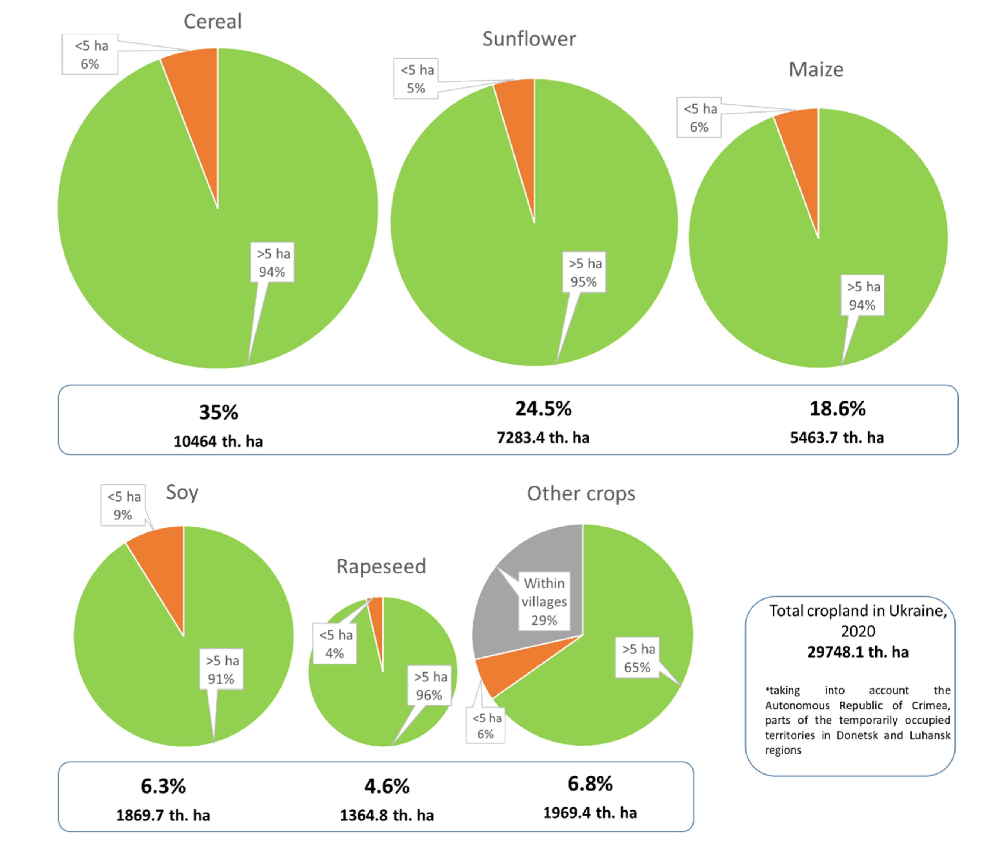
2. Study Area
3. Data
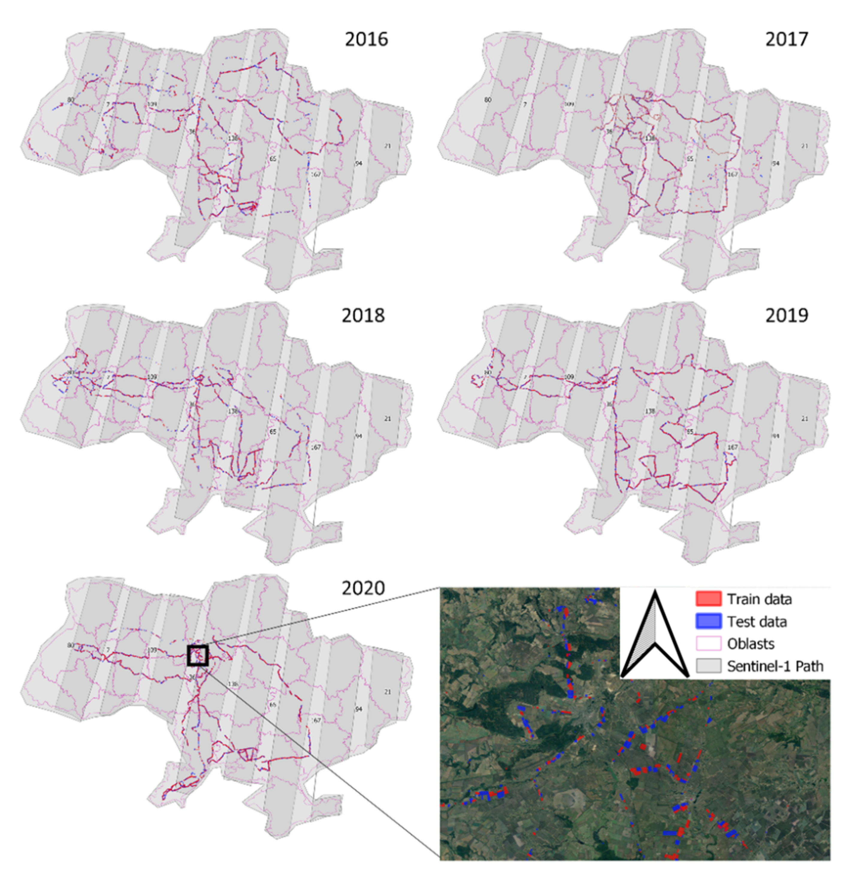
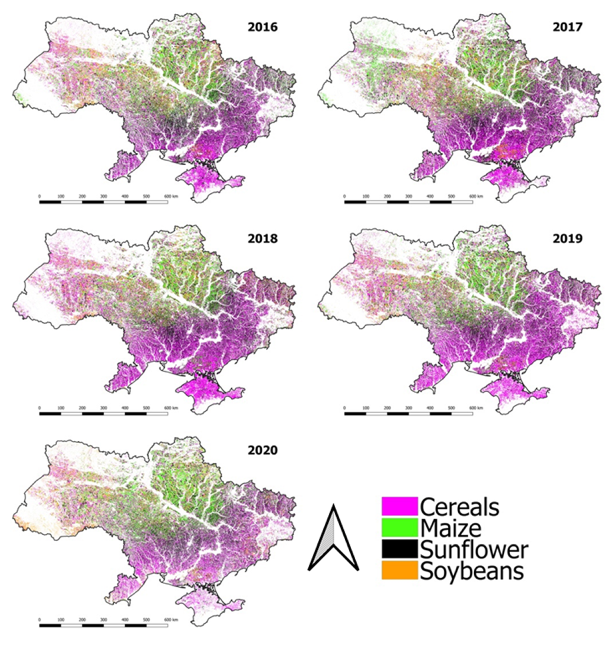
3.1. Crop Classification Maps
3.2. Vegetation Indices
4. Methodology
4.1. Regression Analysis of Crop Rotation
4.2. Model A1 with Binary Crop Rotation Features and Analysis for Five Years
4.3. Model A2 and A3 with Derived Regressors
4.4. Model B for Three-Year Crop Rotation Analysis out of Five Years
4.5. Potential of Sentinel and Landsat Data Usage
5. Results
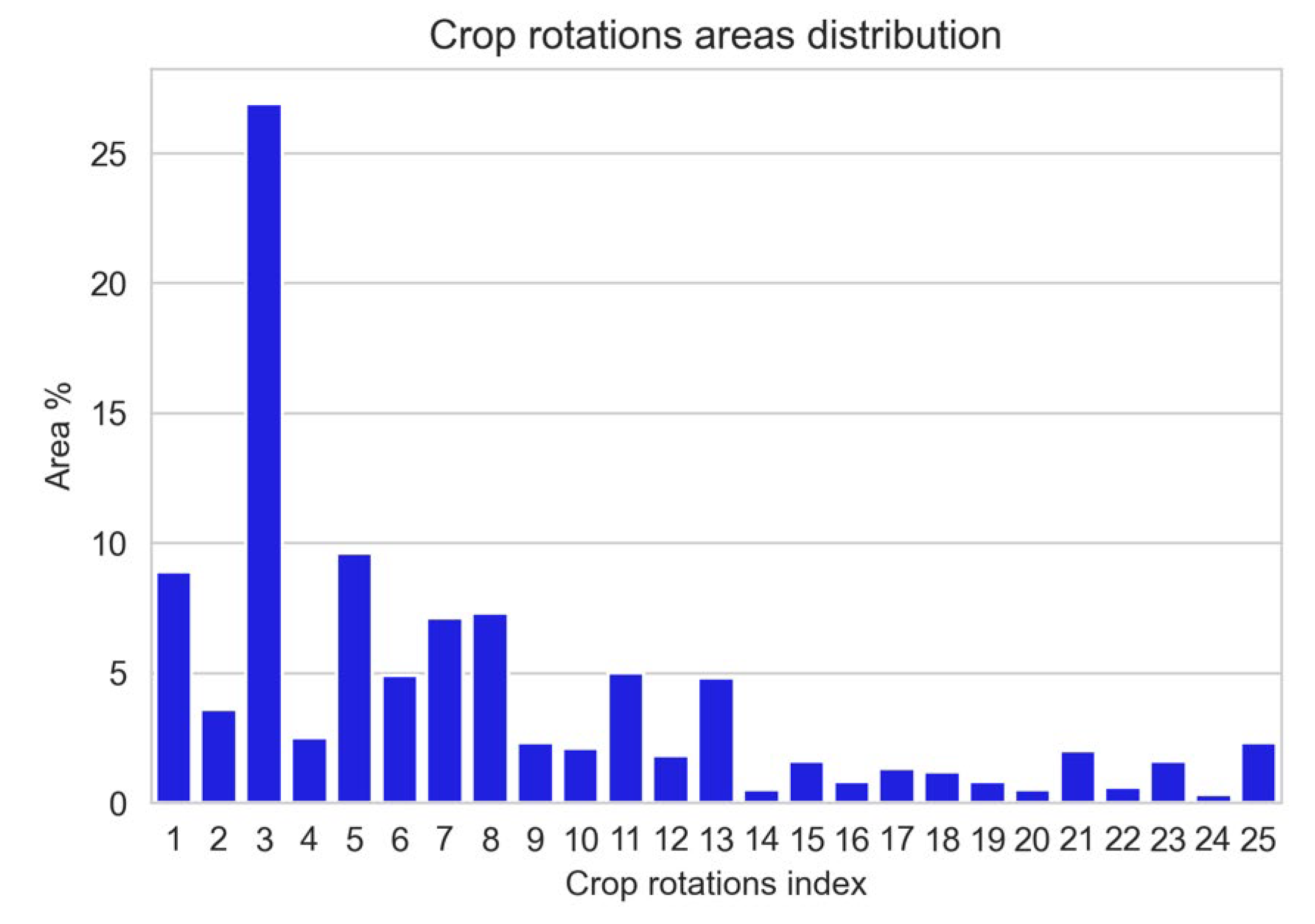
5.1. Results for Model A1 with Binary Crop Rotation Features for Five Years
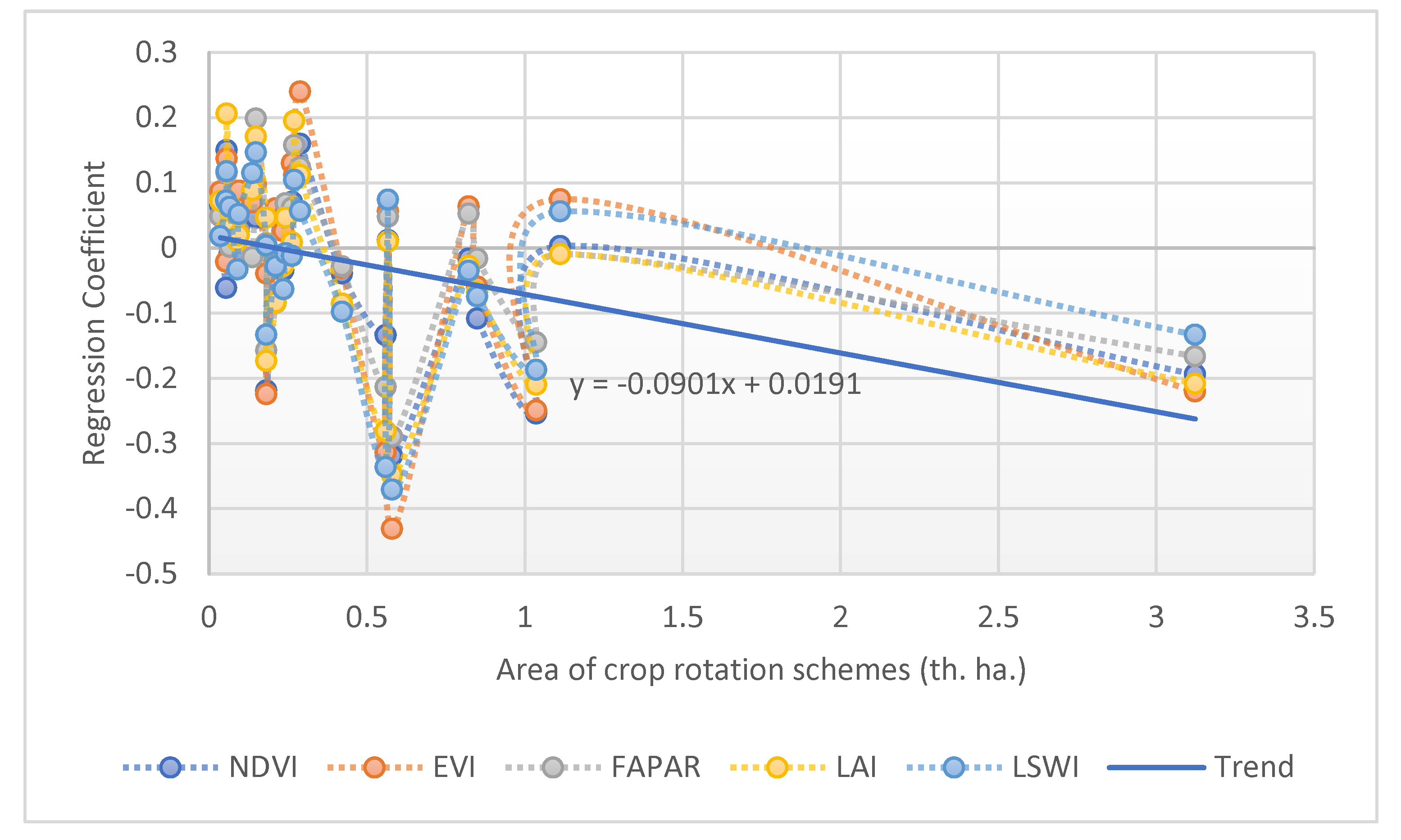
5.2. Results for A2 and A3 Models with Derived Regressors
5.3. Results for Model B for Three Years of Crop Rotation out of Five Years
6. Discussion
6.1. Crop Classification Maps Time Series
6.2. Crop Classification Accuracy
6.3. Crop Rotation Valuation Drawbacks
7. Conclusions
Author Contributions
Funding
Institutional Review Board Statement
Informed Consent Statement
Data Availability Statement
Conflicts of Interest
References
- Zuber, S.M.; Behnke, G.D.; Nafziger, E.D.; Villamil, M.B. Carbon and nitrogen content of soil organic matter and microbial biomass under long-term crop rotation and tillage in Illinois, USA. Agriculture 2018, 8, 37. [Google Scholar] [CrossRef] [Green Version]
- Yang, L.; Song, M.; Zhu, A.-X.; Qin, C.; Zhou, C.; Qi, F.; Li, X.; Chen, Z.; Gao, B. Predicting soil organic carbon content in croplands using crop rotation and Fourier transform decomposed variables. Geoderma 2019, 340, 289–302. [Google Scholar] [CrossRef]
- Maillard, É.; McConkey, B.G.; Luce, M.S.; Angers, D.A.; Fan, J. Crop rotation, tillage system, and precipitation regime effects on soil carbon stocks over 1 to 30 years in Saskatchewan, Canada. Soil Tillage Res. 2018, 177, 97–104. [Google Scholar] [CrossRef]
- McCallum, I.; Montzka, C.; Bayat, B.; Kollet, S.; Kolotii, A.; Kussul, N.; Lavreniuk, M.; Lehmann, A.; Maso, J.; Mazzetti, P.; et al. Developing food, water and energy nexus workflows. Int. J. Digit. Earth 2020, 13, 299–308. [Google Scholar] [CrossRef]
- Bai, Z.G.; Dent, D.L.; Olsson, L.; Schaepman, M.E. Proxy global assessment of land degradation. Soil Use Manag. 2008, 24, 223–234. [Google Scholar] [CrossRef]
- Kussul, N.; Kolotii, A.; Shelestov, A.; Yailymov, B.; Lavreniuk, M. Land degradation estimation from global and national satellite based datasets within UN program. In Proceedings of the 2017 9th IEEE International Conference on Intelligent Data Acquisition and Advanced Computing Systems: Technology and Applications (IDAACS), Bucharest, Romania, 21–23 September 2017; Volume 1, pp. 383–386. [Google Scholar]
- Wang, T.; Giuliani, G.; Lehmann, A.; Jiang, Y.; Shao, X.; Li, L.; Zhao, H. Supporting SDG 15, Life on Land: Identifying the Main Drivers of Land Degradation in Honghe Prefecture, China, between 2005 and 2015. ISPRS Int. J. Geo-Inf. 2020, 9, 710. [Google Scholar] [CrossRef]
- Nhemachena, C.; Matchaya, G.; Nhemachena, C.R.; Karuaihe, S.; Muchara, B.; Nhlengethwa, S. Measuring baseline agriculture-related sustainable development goals index for Southern Africa. Sustainability 2018, 10, 849. [Google Scholar] [CrossRef] [Green Version]
- Kussul, N.; Lavreniuk, M.; Kolotii, A.; Skakun, S.; Rakoid, O.; Shumilo, L. A workflow for Sustainable Development Goals indicators assessment based on high-resolution satellite data. Int. J. Digit. Earth 2020, 13, 309–321. [Google Scholar] [CrossRef]
- Dubovyk, O. The role of Remote Sensing in land degradation assessments: Opportunities and challenges. Eur. J. Remote Sens. 2017, 50, 601–613. [Google Scholar] [CrossRef]
- Sims, N.C.; England, J.R.; Newnham, G.J.; Alexander, S.; Green, C.; Minelli, S.; Held, A. Developing good practice guidance for estimating land degradation in the context of the United Nations Sustainable Development Goals. Environ. Sci. Policy 2019, 92, 349–355. [Google Scholar] [CrossRef]
- Hosseini, M.; McNairn, H.; Mitchell, S.; Robertson, L.D.; Davidson, A.; Ahmadian, N.; Bhattacharya, A.; Borg, E.; Conrad, C.; Dabrowska-Zielinska, K.; et al. A comparison between support vector machine and water cloud model for estimating crop leaf area index. Remote Sens. 2021, 13, 1348. [Google Scholar] [CrossRef]
- Kussul, N.; Lavreniuk, M.; Shumilo, L.; Kolotii, A. Nexus Approach for Calculating SDG Indicator 2.4. 1 Using Remote Sensing and Biophysical Modeling. In Proceedings of the IGARSS 2019-2019 IEEE International Geoscience and Remote Sensing Symposium, Yokohama, Japan, 28 July–2 August 2019; pp. 6425–6428. [Google Scholar]
- Chandrasekar, K.; Sesha Sai, M.V.R.; Roy, P.S.; Dwevedi, R.S. Land Surface Water Index (LSWI) response to rainfall and NDVI using the MODIS Vegetation Index product. Int. J. Remote Sens. 2010, 31, 3987–4005. [Google Scholar] [CrossRef]
- Han, W.; Yang, Z.; Di, L.; Mueller, R. CropScape: A Web service based application for exploring and disseminating US conterminous geospatial cropland data products for decision support. Comput. Electron. Agric. 2012, 84, 111–123. [Google Scholar] [CrossRef]
- Johnson, D.M.; Mueller, R. Pre-and within-season crop type classification trained with archival land cover information. Remote Sens. Environ. 2021, 264, 112576. [Google Scholar] [CrossRef]
- Inan, H.I.; Sagris, V.; Devos, W.; Milenov, P.; Van Oosterom, P.; Zevenbergen, J. Data model for the collaboration between land administration systems and agricultural land parcel identification systems. J. Environ. Manag. 2010, 91, 2440–2454. [Google Scholar] [CrossRef] [Green Version]
- Defourny, P.; Bontemps, S.; Bellemans, N.; Cara, C.; Dedieu, G.; Guzzonato, E.; Hagolle, O.; Inglada, J.; Nicola, L.; Rabaute, T.; et al. Near real-time agriculture monitoring at national scale at parcel resolution: Performance assessment of the Sen2-Agri automated system in various cropping systems around the world. Remote Sens. Environ. 2019, 221, 551–568. [Google Scholar] [CrossRef]
- Sarvia, F.; Xausa, E.; Petris, S.D.; Cantamessa, G.; Borgogno-Mondino, E. A Possible Role of Copernicus Sentinel-2 Data to Support Common Agricultural Policy Controls in Agriculture. Agronomy 2021, 11, 110. [Google Scholar] [CrossRef]
- d’Andrimont, R.; Verhegghen, A.; Lemoine, G.; Kempeneers, P.; Meroni, M.; van der Velde, M. From parcel to continental scale--A first European crop type map based on Sentinel-1 and LUCAS Copernicus in-situ observations. Remote Sens. Environ. 2021, 266, 112708. [Google Scholar] [CrossRef]
- Kussul, N.; Lavreniuk, M.; Skakun, S.; Shelestov, A. Deep learning classification of land cover and crop types using remote sensing data. IEEE Geosci. Remote Sens. Lett. 2017, 14, 778–782. [Google Scholar] [CrossRef]
- Kussul, N.; Lavreniuk, M.; Shumilo, L. Deep Recurrent Neural Network for Crop Classification Task Based on Sentinel-1 and Sentinel-2 Imagery. In Proceedings of the IGARSS 2020–2020 IEEE International Geoscience and Remote Sensing Symposium, Waikoloa, HI, USA, 26 September–2 October 2020; pp. 6914–6917. [Google Scholar]
- Shelestov, A.; Lavreniuk, M.; Kussul, N.; Novikov, A.; Skakun, S. Exploring Google Earth Engine platform for big data processing: Classification of multi-temporal satellite imagery for crop mapping. Front. Earth Sci. 2017, 5, 17. [Google Scholar] [CrossRef] [Green Version]
- Monitoring EU Agri-Food Trade: Developments January–May 2020. Available online: https://ec.europa.eu/info/sites/default/files/food-farming-fisheries/trade/documents/monitoring-agri-food-trade_may2020_en.pdf (accessed on 15 February 2022).
- Irrigation and Drainage Strategy in Ukraine until 2030. Available online: http://www.fao.org/faolex/results/details/en/c/LEX-FAOC190984/ (accessed on 15 February 2022).
- Ukraine Common Country Analysis. Available online: https://ukraine.un.org/sites/default/files/2021-05/UN%20CCA%20Ukraine_April%202021%20%281%29.pdf (accessed on 15 February 2022).
- Kogan, F.; Adamenko, T.; Guo, W. Global and regional drought dynamics in the climate warming era. Remote Sens. Lett. 2013, 4, 364–372. [Google Scholar] [CrossRef]
- Kogan, F.; Kussul, N.; Adamenko, T.; Skakun, S.; Kravchenko, O.; Kryvobok, O.; Shelestov, A.; Kolotii, A.; Kussul, O.; Lavrenyuk, A. Winter wheat yield forecasting in Ukraine based on Earth observation, meteorological data and biophysical models. Int. J. Appl. Earth Obs. Geoinf. 2013, 23, 192–203. [Google Scholar] [CrossRef]
- Fileccia, T.; Guadagni, M.; Hovhera, V.; Bernoux, M. Ukraine: Soil Fertility to Strengthen Climate Resilience; Food and Agriculture Organization of the United Nations: Rome, Italy; Available online: http://www.fao.org/3/a-i3905e.pdf (accessed on 15 February 2022).
- Sobolev, D. Oilseeds and Products Annual. USDA FAS: Kyiv, Ukraine. Available online: https://apps.fas.usda.gov/newgainapi/api/Report/DownloadReportByFileName?fileName=Oilseeds%20and%20Products%20Annual_Kyiv_Ukraine_04-15-2020 (accessed on 15 February 2022).
- Kussul, N.; Lavreniuk, M.; Shelestov, A.; Skakun, S. Crop inventory at regional scale in Ukraine: Developing in season and end of season crop maps with multi-temporal optical and SAR satellite imagery. Eur. J. Remote Sens. 2018, 51, 627–636. [Google Scholar] [CrossRef] [Green Version]
- Resolution of the Cabinet of Ministers of Ukraine, 11 February 2010, Nr 164. Available online: https://zakon.rada.gov.ua/laws/show/164-2010-%D0%BF#Text (accessed on 15 February 2022).
- Shelestov, A.; Lavreniuk, M.; Vasiliev, V.; Shumilo, L.; Kolotii, A.; Yailymov, B.; Kussul, H.; Yailymova, H. Cloud approach to automated crop classification using Sentinel-1 imagery. IEEE Trans. Big Data 2019, 6, 572–582. [Google Scholar] [CrossRef]
- Kussul, N.; Shelestov, A.; Yailymova, H.; Yailymov, B.; Lavreniuk, M.; Ilyashenko, M. Satellite Agricultural Monitoring in Ukraine at Country Level: World Bank Project. In Proceedings of the IGARSS 2020-2020 IEEE International Geoscience and Remote Sensing Symposium, Waikoloa, HI, USA, 26 September–2 October 2020; pp. 1050–1053. [Google Scholar]
- Cox, D.R.; Wermuth, N. Multivariate Dependencies: Models, Analysis and Interpretation. Chapman and Hall/CRC: London, UK, 2014. [Google Scholar]
- Sureiman, O.; Mangera, C.M. F-test of overall significance in regression analysis simplified. J. Pract. Cardiovasc. Sci. 2020, 6, 116. [Google Scholar] [CrossRef]
- Marquardt, D.W.; Snee, R.D. Ridge regression in practice. Am. Stat. 1975, 29, 3–20. [Google Scholar]
- Pasqualotto, N.; Delegido, J.; Van Wittenberghe, S.; Rinaldi, M.; Moreno, J. Multi-crop green LAI estimation with a new simple Sentinel-2 LAI Index (SeLI). Sensors 2019, 19, 904. [Google Scholar] [CrossRef] [PubMed] [Green Version]
- Claverie, M.; Ju, J.; Masek, J.G.; Dungan, J.L.; Vermote, E.F.; Roger, J.-C.; Skakun, S.V.; Justice, C. The Harmonized Landsat and Sentinel-2 surface reflectance data set. Remote Sens. Environ. 2018, 219, 145–161. [Google Scholar] [CrossRef]
- Skakun, S.; Vermote, E.; Franch, B.; Roger, J.C.; Kussul, N.; Ju, J.; Masek, J. Winter wheat yield assessment from Landsat 8 and Sentinel-2 data: Incorporating surface reflectance, through phenological fitting, into regression yield models. Remote Sens. 2019, 11, 1768. [Google Scholar] [CrossRef] [Green Version]
- Rubel, O.; Lukin, V.; Rubel, A.; Egiazarian, K. Prediction of Lee filter performance for Sentinel-1 SAR images. Electron. Imaging 2020, 9, 371. [Google Scholar] [CrossRef]
- Veloso, A.; Mermoz, S.; Bouvet, A.; Le Toan, T.; Planells, M.; Dejoux, J.F.; Ceschia, E. Understanding the temporal behavior of crops using Sentinel-1 and Sentinel-2-like data for agricultural applications. Remote Sens. Environ. 2017, 199, 415–426. [Google Scholar] [CrossRef]
- Filgueiras, R.; Mantovani, E.C.; Althoff, D.; Fernandes Filho, E.I.; Cunha, F.F.D. Crop NDVI monitoring based on sentinel 1. Remote Sens. 2019, 11, 1441. [Google Scholar] [CrossRef] [Green Version]
- Benesty, J.; Chen, J.; Huang, Y.; Cohen, I. Pearson correlation coefficient. In Noise Reduction in Speech Processing; Springer: Berlin/Heidelberg, Germany, 2009; pp. 1–4. [Google Scholar]
- Helland, I.S. On the interpretation and use of R2 in regression analysis. Biometrics 1987, 43, 61–69. [Google Scholar] [CrossRef]


| Class | 2016 | 2017 | 2018 | 2019 | 2020 | |||||
|---|---|---|---|---|---|---|---|---|---|---|
| tr | tt | tr | tt | tr | tt | tr | tt | tr | tt | |
| Artificial | 68 | 67 | 68 | 67 | 164 | 164 | 222 | 223 | 244 | 237 |
| Bare land | 57 | 57 | 54 | 54 | 81 | 80 | 135 | 115 | 138 | 122 |
| Cereals | 1108 | 1106 | 586 | 586 | 1146 | 1146 | 1797 | 1776 | 1911 | 1896 |
| Forest | 338 | 338 | 342 | 341 | 666 | 665 | 223 | 224 | 297 | 291 |
| Grassland | 399 | 399 | 272 | 272 | 651 | 650 | 888 | 866 | 965 | 957 |
| Maize | 514 | 513 | 344 | 344 | 486 | 486 | 576 | 566 | 855 | 850 |
| Peas | 16 | 16 | 25 | 24 | 38 | 38 | 37 | 34 | 61 | 55 |
| Soybeans | 273 | 272 | 191 | 190 | 325 | 324 | 373 | 367 | 389 | 382 |
| Sugar beet | 30 | 29 | 20 | 19 | 69 | 69 | 36 | 29 | 36 | 30 |
| Sunflower | 823 | 822 | 596 | 595 | 876 | 875 | 690 | 681 | 794 | 790 |
| Water | 88 | 88 | 96 | 96 | 240 | 240 | 351 | 327 | 350 | 340 |
| Wetland | 24 | 24 | 35 | 35 | 66 | 66 | 107 | 114 | 133 | 119 |
| Winter rapeseed | 94 | 94 | 107 | 106 | 196 | 195 | 288 | 278 | 273 | 265 |
| Total | 3832 | 3825 | 2736 | 2729 | 5004 | 4998 | 5723 | 5600 | 6446 | 6334 |
| Class | Classification Accuracies (%) | ||||||||||||||
|---|---|---|---|---|---|---|---|---|---|---|---|---|---|---|---|
| 2016 | 2017 | 2018 | 2019 | 2020 | |||||||||||
| UA | PA | F1 | UA | PA | F1 | UA | PA | F1 | UA | PA | F1 | UA | PA | F1 | |
| Artificial | 73.1 | 77.2 | 75.0 | 69.0 | 71.7 | 70.3 | 66.6 | 95.0 | 78.3 | 66.4 | 96.4 | 78.7 | 71.5 | 88.5 | 79.1 |
| Bare land | 58.2 | 63.5 | 60.0 | 55.9 | 66.6 | 60.8 | 90.7 | 67.5 | 77.4 | 61.0 | 67.6 | 64.1 | 84.1 | 60.6 | 70.4 |
| Cereals | 92.0 | 88.1 | 90.0 | 97.3 | 96.5 | 96.9 | 99.0 | 98.7 | 98.8 | 99.1 | 98.5 | 98.8 | 94.5 | 92.2 | 93.3 |
| Forest | 96.9 | 99.3 | 98.1 | 99.2 | 98.2 | 98.7 | 99.7 | 99.8 | 99.8 | 83.4 | 99.2 | 90.6 | 85.5 | 99.8 | 92.1 |
| Grassland | 72.9 | 89.1 | 80.2 | 76.2 | 94.2 | 84.3 | 93.5 | 95.9 | 94.7 | 73.6 | 96.7 | 83.6 | 80.5 | 95.8 | 87.5 |
| Maize | 93.4 | 92.6 | 93.0 | 90.3 | 94.1 | 92.1 | 97.7 | 96.2 | 96.9 | 98.4 | 97.6 | 98.0 | 95.4 | 96.8 | 96.1 |
| Peas | 59.0 | 88.8 | 70.9 | 96.8 | 87.2 | 91.8 | 91.4 | 94.5 | 92.9 | 88.4 | 64.1 | 74.3 | 80.7 | 91.6 | 85.8 |
| Soybeans | 81.6 | 83.4 | 82.5 | 92.5 | 73.0 | 81.6 | 90.5 | 94.2 | 92.3 | 93.1 | 93.6 | 93.3 | 87.8 | 83.9 | 85.8 |
| Sugar beet | 90.9 | 96.6 | 93.6 | 99.8 | 97.5 | 98.6 | 96.4 | 94.6 | 95.5 | 96.6 | 99.3 | 97.9 | 93.3 | 78.7 | 85.4 |
| Sunflower | 94.3 | 94.3 | 94.3 | 94.2 | 97.1 | 95.6 | 98.0 | 98.1 | 98.0 | 98.7 | 98.8 | 98.7 | 96.8 | 97.0 | 96.9 |
| Water | 80.2 | 98.9 | 88.6 | 99.7 | 98.7 | 99.2 | 99.9 | 99.9 | 99.0 | 99.0 | 98.2 | 99.1 | 99.0 | 99.0 | 99.0 |
| Wetland | 77.1 | 77.6 | 77.3 | 83.8 | 49.8 | 62.5 | 85.1 | 64.4 | 73.3 | 88.5 | 81.6 | 84.9 | 86.2 | 86.4 | 86.3 |
| Winter rapeseed | 91.7 | 76.8 | 83.6 | 95.8 | 98.3 | 97.0 | 99.7 | 98.5 | 99.1 | 98.1 | 99.1 | 98.1 | 96.7 | 94.5 | 95.6 |
| OA | 88.3 | 91.0 | 97.3 | 96.2 | 91.6 | ||||||||||
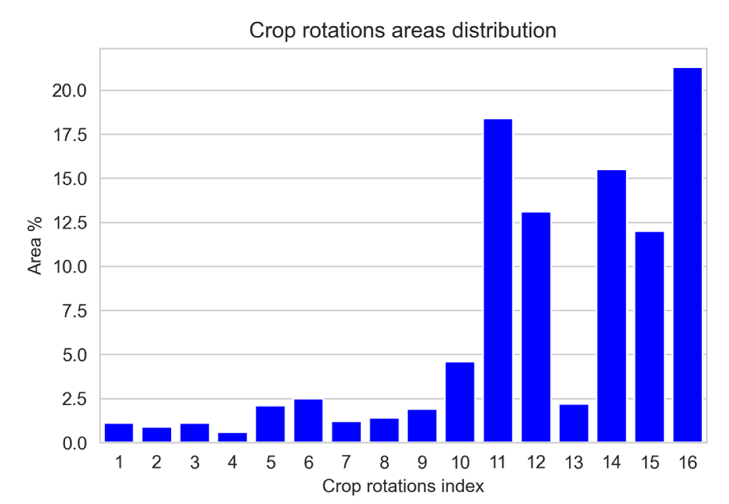
| Index | Binary Representation | 2020 | 2019 | 2018 | 2017 | 2016 |
|---|---|---|---|---|---|---|
| 1 | 11111 | sf | sf | sf | sf | sf |
| 2 | 11110 | sf | sf | sf | sf | nsf |
| 3 | 11101 | sf | sf | sf | nsf | sf |
| 4 | 11100 | sf | sf | sf | nsf | nsf |
| 5 | 11011 | sf | sf | nsf | sf | sf |
| 6 | 11010 | sf | sf | nsf | sf | nsf |
| 7 | 11001 | sf | sf | nsf | nsf | sf |
| 8 | 11000 | sf | sf | nsf | nsf | nsf |
| 9 | 10111 | sf | nsf | sf | sf | sf |
| 10 | 10110 | sf | nsf | sf | sf | nsf |
| 11 | 10101 | sf | nsf | sf | nsf | sf |
| 12 | 10100 | sf | nsf | sf | nsf | nsf |
| 13 | 10011 | sf | nsf | nsf | sf | sf |
| 14 | 10010 | sf | nsf | nsf | sf | nsf |
| 15 | 10001 | sf | nsf | nsf | nsf | sf |
| 16 | 10000 | sf | nsf | nsf | nsf | nsf |
| Index | 2020\2019\2018 | 2019\2018\2017 | 2018\2017\2016 |
|---|---|---|---|
| 1 | Sunflower | Cereals | Cereals |
| 2 | Sunflower | Cereals | Maize |
| 3 | Sunflower | Cereals | Sunflower |
| 4 | Sunflower | Cereals | Soybeans |
| 5 | Sunflower | Cereals | Other |
| 6 | Sunflower | Maize | Cereals |
| 7 | Sunflower | Maize | Maize |
| 8 | Sunflower | Maize | Sunflower |
| 9 | Sunflower | Maize | Soybeans |
| 10 | Sunflower | Maize | Other |
| 11 | Sunflower | Sunflower | Cereals |
| 12 | Sunflower | Sunflower | Maize |
| 13 | Sunflower | Sunflower | Sunflower |
| 14 | Sunflower | Sunflower | Soybeans |
| 15 | Sunflower | Sunflower | Other |
| 16 | Sunflower | Soybeans | Cereals |
| 17 | Sunflower | Soybeans | Maize |
| 18 | Sunflower | Soybeans | Sunflower |
| 19 | Sunflower | Soybeans | Soybeans |
| 20 | Sunflower | Soybeans | Other |
| 21 | Sunflower | Other | Cereals |
| 22 | Sunflower | Other | Maize |
| 23 | Sunflower | Other | Sunflower |
| 24 | Sunflower | Other | Soybeans |
| 25 | Sunflower | Other | Other |
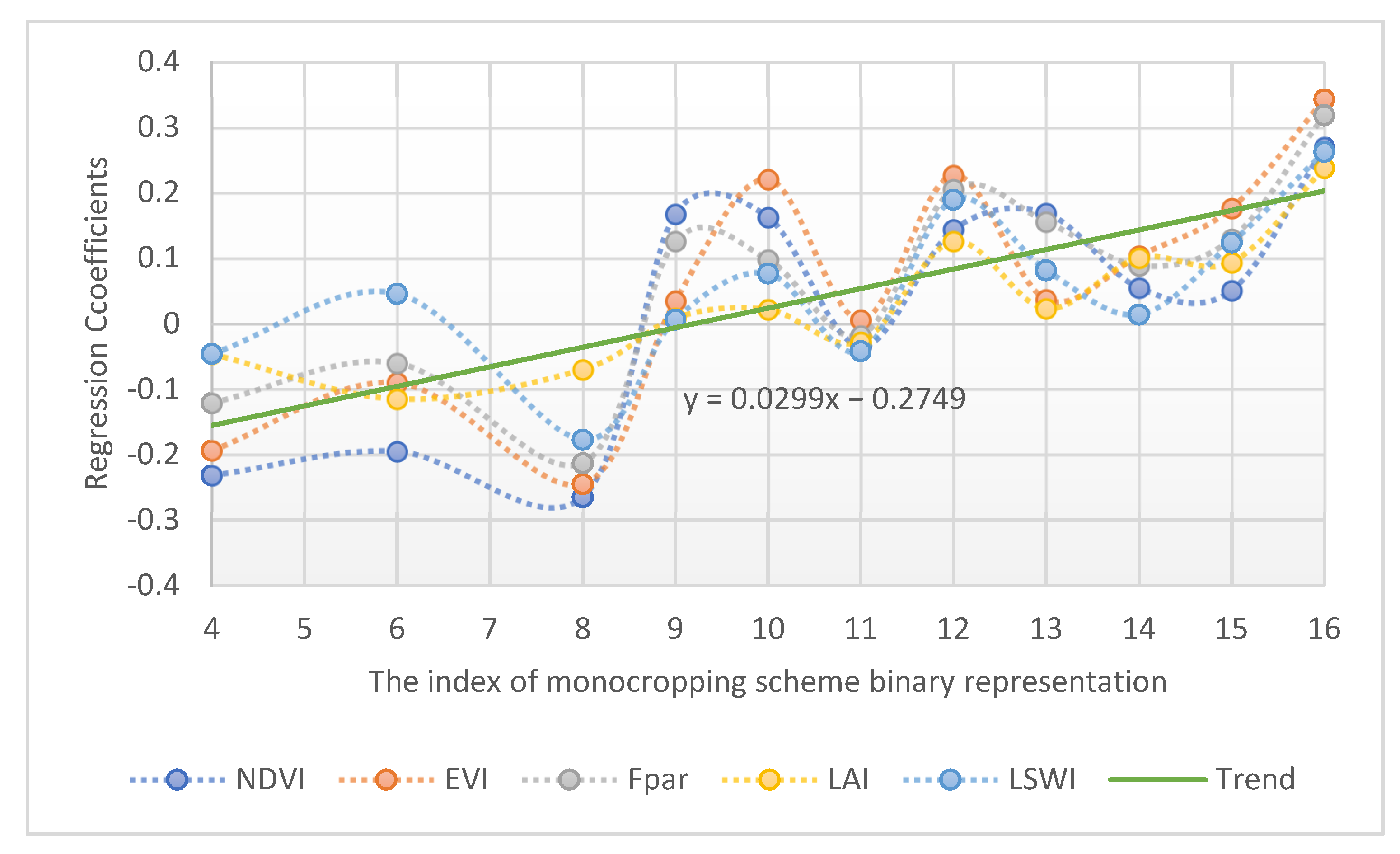
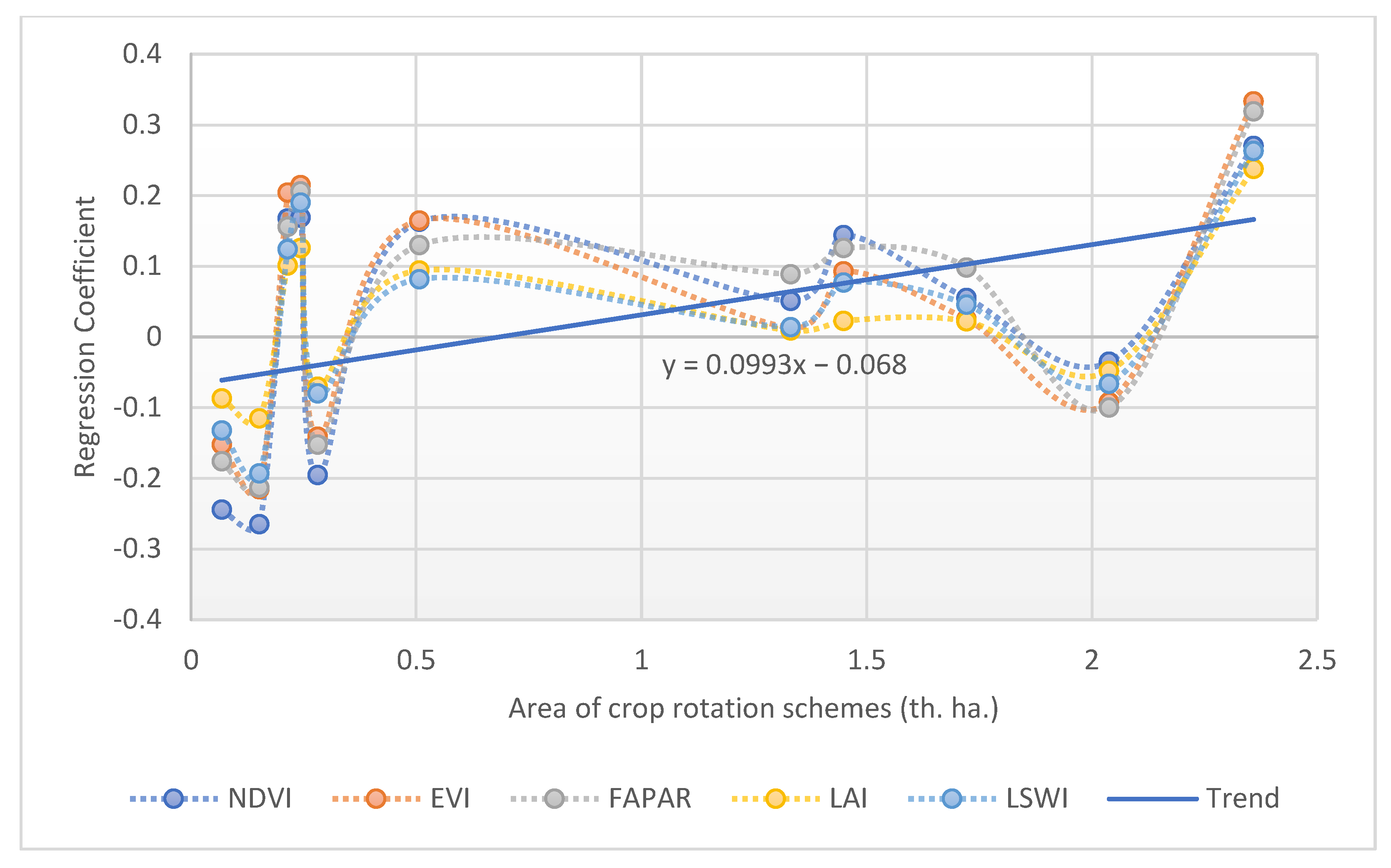
| Binary Representation | Crop Rotation | NDVI | EVI | FAPAR | LAI | LSWI |
|---|---|---|---|---|---|---|
| 11111 | sf-sf-sf-sf-sf | 0.041 * | −0.032 * | −0.09 * | −0.047 * | −0.068 * |
| 11110 | sf-sf-sf-sf-nsf | −0.026 * | −0.158 * | −0.176 * | −0.065 * | −0.132 * |
| 11101 | sf-sf-sf-nsf-sf | −0.025 ** | −0.097 * | −0.1 * | −0.048 * | −0.08 * |
| 11100 | sf-sf-sf-nsf-nsf | −0.232 *** | −0.194 *** | −0.121 *** | −0.046 *** | −0.046 *** |
| 11011 | sf-sf-nsf-sf-sf | −0.244 * | −0.192 * | −0.193 * | −0.105 * | −0.193 * |
| 11010 | sf-sf-nsf-sf-nsf | −0.195 *** | −0.09 *** | −0.06 *** | −0.115 *** | 0.046 *** |
| 11001 | sf-sf-nsf-nsf-sf | −0.04 ** | −0.143 * | −0.152 ** | −0.087 * | −0.066 ** |
| 11000 | sf-sf-nsf-nsf-nsf | −0.265 *** | −0.245 *** | −0.213 *** | −0.07 *** | −0.177 *** |
| 10111 | sf-nsf-sf-sf-sf | 0.168 *** | 0.035 ** | 0.126 ** | 0.009 ** | 0.007 *** |
| 10110 | sf-nsf-sf-sf-nsf | 0.163 *** | 0.221 *** | 0.098 *** | 0.022 *** | 0.077 *** |
| 10101 | sf-nsf-sf-nsf-sf | −0.035 *** | 0.006 *** | −0.018 *** | −0.028 *** | −0.042 *** |
| 10100 | sf-nsf-sf-nsf-nsf | 0.144 *** | 0.227 *** | 0.206 *** | 0.126 *** | 0.19 *** |
| 10011 | sf-nsf-nsf-sf-sf | 0.169 *** | 0.037 *** | 0.156 *** | 0.023 *** | 0.082 *** |
| 10010 | sf-nsf-nsf-sf-nsf | 0.055 *** | 0.104 *** | 0.089 *** | 0.101 *** | 0.014 *** |
| 10001 | sf-nsf-nsf-nsf-sf | 0.051 *** | 0.177 *** | 0.13 *** | 0.094 *** | 0.124 *** |
| 10000 | sf-nsf-nsf-nsf-nsf | 0.27 *** | 0.343 *** | 0.319 *** | 0.238 *** | 0.263 *** |
| Crop Rotation | NDVI | EVI | LAI | FAPAR | LSWI |
|---|---|---|---|---|---|
| Sunflower-Cereals-Cereals | −0.254 *** | −0.249 *** | −0.145 *** | −0.21 *** | −0.187 *** |
| Sunflower-Cereals-Maize | −0.039 *** | −0.031 *** | −0.028 *** | −0.085 *** | −0.098 *** |
| Sunflower-Cereals-Sunflower | −0.194 *** | −0.22 *** | −0.166 *** | −0.208 *** | −0.133 *** |
| Sunflower-Cereals-Soybeans | 0.16 *** | 0.24 *** | 0.124 *** | 0.112 *** | 0.057 *** |
| Sunflower-Cereals-Other | 0.003 *** | 0.075 *** | −0.009 *** | −0.009 *** | 0.056 *** |
| Sunflower-Maize-Cereals | 0.012 *** | 0.056 *** | 0.048 *** | 0.01 *** | 0.074 *** |
| Sunflower-Maize-Maize | −0.016 *** | 0.064 *** | 0.053 *** | −0.027 *** | −0.035 *** |
| Sunflower-Maize-Sunflower | −0.108 *** | −0.059 *** | −0.016 *** | −0.067 *** | −0.074 *** |
| Sunflower-Maize-Soybeans | 0.071 *** | 0.13 *** | 0.062 *** | 0.009 *** | −0.012 *** |
| Sunflower-Maize-Other | 0.044 *** | 0.055 *** | 0.069 *** | 0.047 *** | −0.008 *** |
| Sunflower-Sunflower-Cereals | −0.319 *** | −0.431 *** | −0.289 *** | −0.348 *** | −0.371 *** |
| Sunflower-Sunflower-Maize | 0.059 *** | 0.061 *** | −0.084 *** | −0.083 *** | −0.028 *** |
| Sunflower-Sunflower-Sunflower | −0.134 *** | −0.313 *** | −0.213 *** | −0.281 *** | −0.336 *** |
| Sunflower-Sunflower-Soybeans | −0.061 *** | −0.021 *** | 0.025 *** | 0.029 *** | 0.073 *** |
| Sunflower-Sunflower-Other | 0.005 *** | −0.039 *** | 0.007 *** | 0.047 *** | 0.004 *** |
| Sunflower-Soybeans-Cereals | −0.012 *** | 0.048 *** | 0.027 *** | 0.011 *** | −0.033 *** |
| Sunflower-Soybeans-Maize | 0.047 *** | 0.098 *** | 0.199 *** | 0.171 *** | 0.147 *** |
| Sunflower-Soybeans-Sunflower | 0.052 *** | 0.07 *** | −0.014 *** | 0.089 *** | 0.115 *** |
| Sunflower-Soybeans-Soybeans | 0.03 *** | 0.088 *** | 0.025 *** | 0.02 *** | 0.052 *** |
| Sunflower-Soybeans-Other | 0.15 *** | 0.137 *** | 0.115 *** | 0.206 *** | 0.118 *** |
| Sunflower-Other-Cereals | −0.034 *** | 0.026 *** | −0.009 *** | −0.027 *** | −0.063 *** |
| Sunflower-Other-Maize | −0.008 *** | 0.03 *** | 0.002 *** | 0.065 *** | 0.063 *** |
| Sunflower-Other-Sunflower | −0.219 *** | −0.224 *** | −0.157 *** | −0.173 *** | −0.133 *** |
| Sunflower-Other-Soybeans | 0.065 *** | 0.087 *** | 0.049 *** | 0.072 *** | 0.018 *** |
| Sunflower-Other-Other | 0.131 *** | 0.112 *** | 0.158 *** | 0.195 *** | 0.105 *** |
| R2 score | 0.31 | 0.39 | 0.44 | 0.4 | 0.21 |
Publisher’s Note: MDPI stays neutral with regard to jurisdictional claims in published maps and institutional affiliations. |
© 2022 by the authors. Licensee MDPI, Basel, Switzerland. This article is an open access article distributed under the terms and conditions of the Creative Commons Attribution (CC BY) license (https://creativecommons.org/licenses/by/4.0/).
Share and Cite
Kussul, N.; Deininger, K.; Shumilo, L.; Lavreniuk, M.; Ali, D.A.; Nivievskyi, O. Biophysical Impact of Sunflower Crop Rotation on Agricultural Fields. Sustainability 2022, 14, 3965. https://doi.org/10.3390/su14073965
Kussul N, Deininger K, Shumilo L, Lavreniuk M, Ali DA, Nivievskyi O. Biophysical Impact of Sunflower Crop Rotation on Agricultural Fields. Sustainability. 2022; 14(7):3965. https://doi.org/10.3390/su14073965
Chicago/Turabian StyleKussul, Nataliia, Klaus Deininger, Leonid Shumilo, Mykola Lavreniuk, Daniel Ayalew Ali, and Oleg Nivievskyi. 2022. "Biophysical Impact of Sunflower Crop Rotation on Agricultural Fields" Sustainability 14, no. 7: 3965. https://doi.org/10.3390/su14073965
APA StyleKussul, N., Deininger, K., Shumilo, L., Lavreniuk, M., Ali, D. A., & Nivievskyi, O. (2022). Biophysical Impact of Sunflower Crop Rotation on Agricultural Fields. Sustainability, 14(7), 3965. https://doi.org/10.3390/su14073965