Identification of Potential Valid Clients for a Sustainable Insurance Policy Using an Advanced Mixed Classification Model

Abstract

Due to the social awareness of risk control, we are witnessing the popularization of the insurance concept and the rapid development of financial insurance. The performance of the insurance industry is highly competitive; thus, in order to develop new and old business from existing clients, information on the renewal of client premiums, purchase of new policies, and new client referrals has become an important research topic in this field. However, based on a review of published literature, few scholars have engaged in relevant research on the above topics by data mining, which motivated the formation of this study, hoping to bridge this gap. We constructed 10 mixed classification prediction models (called Models A–J) using advanced data mining techniques. Moreover, 19 conditional attributes (coded as X1–X19) were selected from the collected insurance client database, plus three different decision attributes (coded as X20–X22): whether to pay the renewal insurance premium, whether to buy a new insurance policy, and whether to introduce new clients. In terms of technical methods, we used two data pretreatment techniques, attribute selection and data discretization, combined with different methods of disassembly in proportion and data cross-validation to conduct data analysis of the collected experimental data set. We also combined and calculated 23 important classification algorithms (or classifiers) in seven different classifications of data mining techniques (i.e., decision tree, Bayes, Function, Lazy, Meta, Mise, and Rule). In terms of the experimental results of insurance data, this study has the following important contributions and findings: (1) finding the best classifier; (2) finding the optimal mixed classification model; (3) determining the best disassembly in proportion; (4) comparing the performance of different disassembly in proportion and data cross-validation methods; (5) determining the important factors influencing the decision attribute “whether to purchase a new insurance policy”, including the time interval to the first purchase, the number of valid policies, the total number of purchased policies, the family salary structure, and gender; and (6) building a knowledge base of decision rules and criteria with the decision tree C4.5 technology, which shall be provided to relevant stakeholders such as insurance dealers and insurance salespeople as a reference for looking for valid clients in the future, and is conducive to the rapid expansion of insurance business. Finally, the important research findings and management implications of this study can serve as a basis for further study of sustainable insurance by academic researchers.

1. Introduction

The present work targets two key issues to address our research points. On one hand, insurance is an important issue for a person or family in financial planning and ensuring that individual assets can be effectively protected when an accident or harm occurs. Common insurance types cover motor vehicles, travel, health, and homes. In terms of comparative advantages, insurance offers wide benefits, including financial security, risk transformation, asset protection, and peace of mind. Thus, in the 21st century, with heightened risk awareness, insurance companies attract clients who pay premiums for guaranteed protection, and risk transfer through insurance planning has become an important tool to mediate consumers’ worries and risk aversion [1]. In particular, in the face of economic recession and depression in recent years worldwide, market transactions have decreased sharply; thus, some problems have emerged concerning insurance policies. For example, do clients continue to pay premiums for an insurance policy? Do they want to buy insurance again? Other issues such as the referral of new clients affect the survival of insurance businesses. These issues provide rationale for exploring the importance of insurance policies, and this is highlighted in this study. Furthermore, there are many benefits that cannot be distributed within the scope of some specific types of health insurance and must instead be purchased separately, such as life insurance. In particular, life insurance can provide people the specific medical care services they need when they fall seriously ill. Currently, the commercial medical insurance of life insurance focuses on its importance and necessity. Thus, life insurance also motivates this research and is highlighted in this study.

The development of the insurance industry previously flourished under the protection of the government until it became increasingly competitive in the face of contemporary economic freedom and globalization [2]. Insurance is the cornerstone of a stable national economy, and finance is the economic indicator of that. Through the era of agriculture, industry, and commerce, and now the era of cloud technology, enterprises strive for innovation in their business models. In the economic development of countries, insurance may be one of the most common conservative tools for individual investment, financial management, and risk protection. Specifically, people’s concept of medical insurance has changed, where prevention is more important than treatment, and the treatment has high recognition; thus, the purchase rate of life insurance, accident insurance, medical insurance, and cancer insurance is increasing year by year. We carried out this study using effective technology, particularly data mining techniques of existing relevant client data, to address the important issues related to life insurance to enable insurance companies to seek out clients who are likely to renew their policies.

Data mining technology can be applied in a variety of fields, such as foodomics [3], classroom learning [4], community resources [5], smart cities [6], bus crash severity [7], and other related fields, but it is rarely applied in the development of insurance sales. In addition, from reviewing the literature on data mining technology, it is found that some effective classifiers appear in various application fields, and their superior performance is welcomed by the industry and academia. There are 23 classifiers in seven classification groups (decision tree, Bayes, Function, Lazy, Meta, Mise, and Rule) used in this study, which already have application evidence in the insurance field, such as in motor insurance [8,9]. Therefore, they were chosen to be used in this study. We used automatic and semi-automatic ways to analyze the existing client insurance data, particularly data mining tools, to investigate, find the unknown data or rules hidden in large amounts of data, sum up useful knowledge, and apply the findings to an actual insurance business to help the insurance companies and identify the most suitable decisions regarding potential client lists. Through the client conditional data, we compiled files, applied classification algorithms, and combined different disassembly in proportion and data cross-validation methods, as well as decision tree classification technology, to predict client re-purchasing, referral of new clients, and clients continuing to pay premiums, and thus to help insurers make the right planning decisions through the experiment and analysis of data and rules. The purposes of this study can be summarized as follows. (1) Use the conditional attributes combined with data mining classification technology to construct an insurance prediction model. (2) Pinpoint the important factors affecting the insurance decision attributes. (3) Output the decision tree diagrams and decisional rules. (4) Evaluate the performance differences of insurance prediction models. (5) Distinguish the optimal model with the best accuracy.

Based on relevant practices and literature, we believe that research on exploring and developing potential insurance clients is beneficial to all the above research purposes. It is interesting to note that, given the limited evidence in the literature, the development of insurance sales is rare in the field of data mining, which emphasizes that the results of this study can apply to different types of industries. Therefore, it is important for this study to establish the development of insurance sales and to attach importance to the experience of research framework. The rest of this paper is organized as follows. Section 2 is an extensive literature review of some of the topics in the insurance field and data mining technology. Section 3 describes the structures and applications of the various mixed classification models proposed. Section 4, Section 5 and Section 6 report the analysis and discussion of the empirical results, as well as the conclusions with future insights and future research directions.

2. Literature Review

This section introduces life insurance, data mining technology, attribute selection methods, data discretization technology, and different important classification algorithms.

2.1. Life Insurance

“Insurance” is derived from the premiums paid by thousands of insured people. Insurance can ameliorate our troubles in the event of loss, and insurance allows us to help others when they experience hardship. Regarding the definition of insurance, it mainly takes the life (life insurance), body (accident insurance), and health (medical insurance) of the “insured” as the subject of insurance. These types of insurance are briefly introduced as follows. (1) Life insurance: the applicant and the insured apply for insurance with an insurance company and pay premiums according to the contract. During the insurance period, if the insured dies, is completely disabled, or reaches a certain age for illness or accident, the insurance company will pay the insurance benefits according to the contract [10]. Plans include whole-life insurance, term life insurance, savings insurance, critical illness insurance, and long-term care insurance. (2) Accident insurance: Insurance against death, total disability, partial disability, and injury caused by external and unexpected accidents not caused by disease [11]. (3) Hospitalization insurance: There are two types of medical insurance for hospitalization due to disease, namely the fixed amount and actual payment within the quota. (4) Cancer insurance: Cancer is the first among the top ten causes of death. When suffering from cancer, patients must receive various types of related treatment and family care, which will have an impact on both individual and family finances. Cancer insurance can make up for the various costs and expenses caused by cancer, especially the income reduction due to hospitalization, to help the patients undergo treatment and recuperation and effectively mitigate the impact on individuals and families [12]. (5) Investment insurance: Includes two accounts—the amount insured and the fund. The insurance company invests various types of funds according to the fund target selected by the insured and the account value in the policy. (6) Annuity insurance: A form of insurance in which the insured pays the premium in a lump sum or installments as agreed upon during the insured’s life or during a specified period.

Relevant studies on insurance have been applied in various fields, such as calculating the policy costs in crisis economy [13], the effect of unemployment rate on dental insurance [14], trust in insurance [15], unemployment insurance [16], and crop insurance [17].

2.2. Data Mining Technology

The process of data mining is similar to mining by workers. It uses various tools to determine the relationship between conditional data, special rules, and valuable information and knowledge through a series of cleaning, sorting, and analysis of mountains of data [18]. Data mining is a tool or method that primarily extracts knowledge from a large amount of data. It is an important competitive advantage of this industry to discover potentially useful resources hidden in massive, incomplete, and fuzzy complex data, and then transform these precious resources into valuable information and knowledge to provide decision-makers with important and appropriate decision tools. Data mining is a core step in the process of knowledge mining. The process of knowledge discovery in database (KDD) selects the target data from a database, cleans and consolidates the data, and then transforms the data format for the process of data mining and result evaluation analysis [19]. Data mining is usually a comprehensive computer science combining databases, artificial intelligence, machine learning, and statistics.

2.3. Attribute Selection Method

Attribute selection is an important part of machine learning to select the best features from the original data with appropriate identification ability, which can not only simplify calculations, but also help in understanding the causal relationship of the problem [20,21]. This method is widely used in many research fields, such as statistical pattern analysis, machine learning, and data mining. Attribute selection has many advantages, including (1) data collection: reducing the resource costs and make the data clear and easy to see; (2) data processing: deleting redundant attributes to make the calculation of model building more efficient; (3) data interpretation: after the attribute selection, improvement of interference prediction results, enhancement of explanatory ability, and acceleration of model derivation and knowledge mining. Attribute selection can help solve the problem of having too much low-value data and too little high-value data, reduce calculation time, improve prediction performance, and better understand the machine learning or pattern recognition applications. Attribute selection is used to search all possible combinations of all attributes in the data set and identify the group of attributes with the best prediction effects.

2.4. Data Discretization Technology

Discretization that may be used for a continuous attribute is a basic pre-processing technology and one of the effective and influential data pre-processing tasks. The purpose is to take the concise data as a category suitable for learning tasks, and convert the digital attributes into discrete data, making it easier for experts to understand [22,23]. There are two discretization methods. First, according to the expert’s personal judgment, the attribute can be changed to the classification interval, as the expert discretization makes it easy to understand the result. Second, to ensure the correctness of the value range, different equations are used to perform the automatic discretization of data cutting. In data mining research, due to the limitations of a large amount of data and resources as well as other reasons, expert discretization cannot show the whole picture of the results, so automatic discretization has become favored by researchers.

2.5. Different and Important Classification Algorithm

Classification is important in data mining to solve problems or classify data. It is aimed at analyzing the data of a training set, establishing models or exploring classification rules, and then classifying other data with these rules. A classification algorithm (or classifier) is when computer scientists map real problems to mathematical problems, design formulas, and then write the formulas into a program language that connects them to the computer so the computer can run programs to calculate the answers [24]. These formulas are called algorithms. Based on previous literature, the decision tree has satisfactory evaluation performance and is an advantageous classification tool. In this study, 23 classifiers are classified into seven classification algorithms by data mining software according to different characteristics. The seven classification algorithms are explained as follows:

• Decision tree: Decision tree is a very popular classification and prediction tool used for data analysis and decision-making assistance; it uses the graph of a tree and the possible results to form a special tree structure for the establishment of a target decision model. Decision tree is used to classify a large number of documents in a regular way that can clearly explain the classification [25]. In this study, the decision tree algorithm is used as a prediction tool for the repurchase, referral, and renewal of insurance premiums, mainly presented as a decision tree graph. Trees in this study mainly include J48 [26], LMT [27], and REP Tree [28] classifiers.
• Bayes: Naïve Bayes (NB) is a statistical classification method. Graphical models are used to represent relationships between attributes [29]. Possible values can be classified and calculated to achieve a complete and reasonable prediction. Bayes in this study include Bayes Net [30] and Naïve Bayes classifiers.
• Function: Logistic regression is one of the models of discretization choice methods, which belongs to the category of multivariate analysis and is a common method of statistical empirical analysis in sociology, biostatistics, quantitative psychology, econometrics, and marketing [31]. Function in this study includes SMO, SGD, Simple Logistic, and SGD Text.
• Lazy: A multi-classifier integration algorithm based on dynamic programming. Lazy is relatively gentle and better than other methods in terms of dynamic adaptability to concepts. It can reasonably adjust the proportion of each classifier in the prediction and achieve better results. Different learning algorithms can also be integrated to complete the new training data. Lazy in this study includes IBK [32], K-Star, and LWL.
• Meta: Group learning. Meta in this study mainly includes Stacking, Vote, and AdaBoostM1 [33].
• Rule: Rule contains a variety of different algorithms, such as JRip, OneR, PART, ZeroR, Decision Table, etc., which have different calculation methods and can be widely used in classification methods of different industries.
• Mise: Other classifiers different from the above six categories belong to Mise, which is represented by InputMappedClassifier in this study.

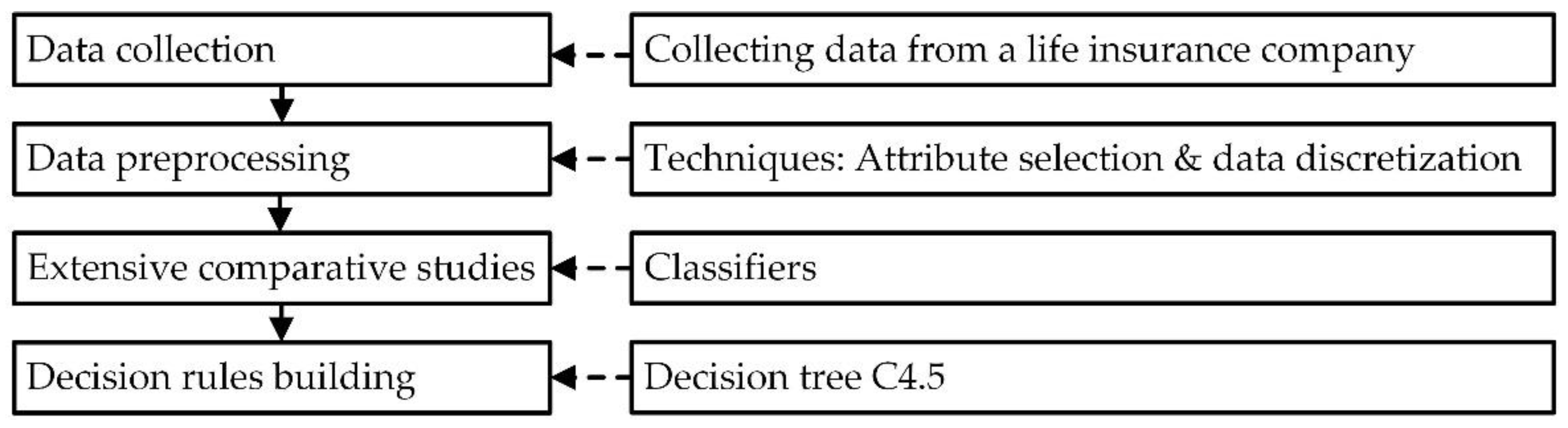
3. Research Methods

This section introduces the framework of the proposed mixed classification model and its research steps and illustrates the process of mining the valid insurance client forecasting model with an example.

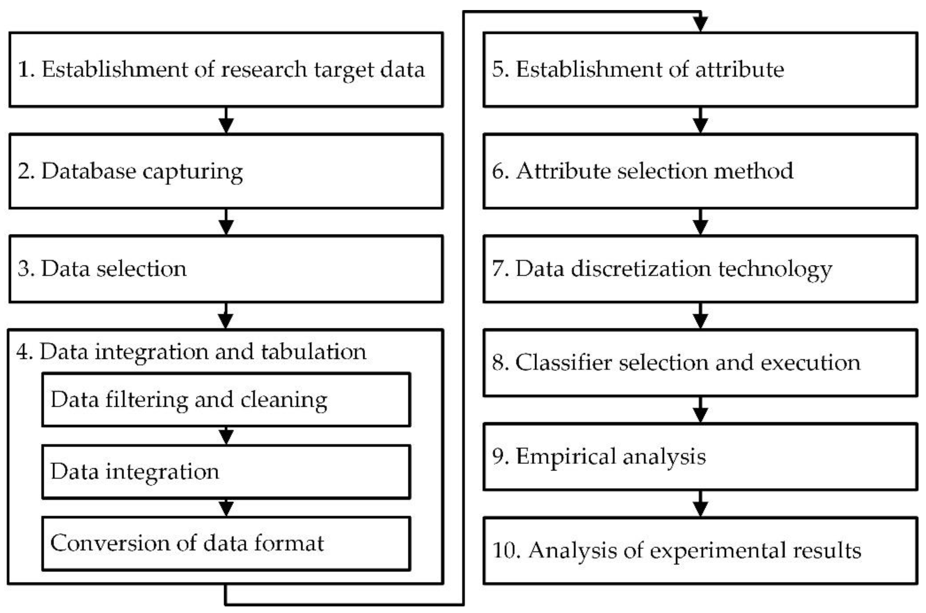
3.1. Research Framework

Based on the data of a life insurance company in Taiwan, we adopted the binary classification method to construct a mixed classification model and used decision tree technology to construct a decision rule knowledge base and carry out its analysis. We first established the research objectives, planned the relevant conditional attribute data required, and then collected the actual data of a life insurance company from 1 August 1997 to 31 December 2017. After the pre-data clearing, the attribute codes were set, and then a spreadsheet was prepared. Then, the file format was converted into Excel CSV as required by the data. Next, data analysis and the decision tree algorithm were carried out through the proposed mixed classification prediction model to determine the decision rules to help insurance companies and insurance salespeople compile valid client lists through the analysis results of decision rules and to help salespeople to achieve twice the results with half the efforts in promoting their insurance business. Figure 1 shows the diagram of methodology in this study. The algorithm of the mixed classification model in this study consists of 10 steps, as shown in the flow chart presented in Figure 2.

3.2. Research Steps of Proposed Mixed Classification Model Algorithm and Example Illustration

The valid insurance client mixed classification prediction model proposed in this study has the following ten key steps, which are described in detail with a practical example as follows.

Step 1: Establishment of research target data.

From expert opinion and discussion, the research direction and relevant data needed were established, data pre-processing (search, collection, and cleaning) was conducted, and then predictive analysis was carried out. This step is a key aspect of knowledge mining. We first established the research direction and determined three different categories of decision attributes and their codes as follows: (1) whether to repurchase a new policy (X20), (2) whether to introduce new clients (X21), and (3) whether to pay the renewal insurance premium (X22).

Step 2: Database capturing.

Next, to enter the database to select and extract the target field, the insurance attribute data of this study were collected from the database of a life insurance company in Taiwan, and the data downloaded were from 1 August 1997 to 31 December 2017. After being cleaned and filtered one by one from the database of the collected objects, the conditional data types required for this study were sorted.

Step 3: Data selection.

According to the contents of downloaded insurance information, the selection of “conditional attribute” mainly referred to the opinions of three insurance experts, and to the whole conditional attribute data. Then, the data belonging to the conditional attributes were cleaned and sorted in advance and integrated into the Excel spreadsheet one by one.

Step 4: Data integration and tabulation.

In the above data summary, there were sub-steps for data filtering, cleaning, integration, and format conversion, which are explained as follows:

• Data filtering and cleaning: Relevant sub-steps include (a) selecting client and policy data from the database, deleting personal privacy data such as name and ID card, and verifying similar repeated data; (b) the number of policies, which was numerical, and the types of insurance, which were classified as life insurance, critical illness insurance, investment insurance, and savings insurance; (c) the total number of policies and the amount of insurance; (d) recording the number of valid policies; (e) calculating time to first purchase; (f) removing redundant, incomplete, or similar repeated conditional attribute data to maintain the integrity and validity of the data and thus improve the accuracy of data mining technology.
• Data integration: Continuing the above steps to check and verify the data to ensure data correctness, and check and confirm whether the setting of each conditional field in the Excel spreadsheet was correct, such as age, total premium, and total insurance amount. Interestingly, because the accuracy and completeness of data are positively correlated with the quantity and quality of data in the data mining, this affects the research results of data mining. Therefore, this step is critical.
• Conversion of data format: According to the data files after integration, 300 useful data points were confirmed and converted into the format files required for the experimental data of this study for further data analysis.

Step 5: Establishment of attributes.

The relevant attributes used in this study were based on the insurance experts’ opinions and literature review, and 19 conditional attributes and three different categories of decision attributes were selected as follows.

• Conditional attributes: Gender, education background, marriage, job nature, whether the spouse is employed, family salary structure, payment method, amount of life insurance, insurance payer, amount of critical illness insurance, whether there is an investment insurance policy, amount of long-term care insurance, premium of long-term care insurance, total number of purchased insurance policies, number of valid policies, time to first purchase, total premium of personal annual valid insurance policy, amount of life insurance/10,000, and total amount of life insurance (including long-term care insurance). Detailed information and codes are shown in Table 1.
• Decision attribute: Three different categories, including whether to repurchase a new insurance policy, whether to introduce new clients, and whether to pay the renewal insurance premium. The binary classification method was used to test and verify the experimental research data. The detailed data are shown in Table 2. In Table 2, “Y” refers to yes, and “N” refers to no.
• Coding: The codes X1, X2, X3...X22 in this study represent the conditional attributes and decision attributes.

Table 1. Conditional attribute data type.

Field	Conditional Attribute	Reference	Data type	Code
1	Gender	[34]	Text	X1
2	Education background	[34]	Text	X2
3	Marriage	[35]	Text	X3
4	Job nature	[36]	Text	X4
5	Whether the spouse is employed	* [By expert]	Text	X5
6	Family salary structure	* [By expert]	Text	X6
7	Payment method	* [By expert]	Numeric	X7
8	Amount of life insurance	[37]	Numeric	X8
9	Insurance payer	* [By expert]	Text	X9
10	Amount of critical illness insurance	[38]	Numeric	X10
11	Whether there is an investment insurance policy	[39]	Text	X11
12	Amount of long-term care insurance	[40]	Numeric	X12
13	Premium of long-term care insurance	[40]	Numeric	X13
14	Total number of purchased policies	* [By expert]	Numeric	X14
15	Number of valid insurance policies	* [By expert]	Numeric	X15
16	Time to first purchase	* [By expert]	Numeric	X16
17	Total premium of personal annual valid insurance policy	* [By expert]	Numeric	X17
18	Amount of life insurance/10,000	[37]	Numeric	X18
19	Total amount of life insurance (including long-term care insurance)	[41,42,43,44]	Numeric	X19

Note: * [By expert] refers to the interviewed results of three insurance experts with consensus.

Table 1. Conditional attribute data type.

Field	Conditional Attribute	Reference	Data type	Code
1	Gender	[34]	Text	X1
2	Education background	[34]	Text	X2
3	Marriage	[35]	Text	X3
4	Job nature	[36]	Text	X4
5	Whether the spouse is employed	* [By expert]	Text	X5
6	Family salary structure	* [By expert]	Text	X6
7	Payment method	* [By expert]	Numeric	X7
8	Amount of life insurance	[37]	Numeric	X8
9	Insurance payer	* [By expert]	Text	X9
10	Amount of critical illness insurance	[38]	Numeric	X10
11	Whether there is an investment insurance policy	[39]	Text	X11
12	Amount of long-term care insurance	[40]	Numeric	X12
13	Premium of long-term care insurance	[40]	Numeric	X13
14	Total number of purchased policies	* [By expert]	Numeric	X14
15	Number of valid insurance policies	* [By expert]	Numeric	X15
16	Time to first purchase	* [By expert]	Numeric	X16
17	Total premium of personal annual valid insurance policy	* [By expert]	Numeric	X17
18	Amount of life insurance/10,000	[37]	Numeric	X18
19	Total amount of life insurance (including long-term care insurance)	[41,42,43,44]	Numeric	X19

Note: * [By expert] refers to the interviewed results of three insurance experts with consensus.

Table 2. Decision attribute binary classification data.

Attribute	Classification
Whether to repurchase the new insurance policy (X20)	Y and N
Whether to introduce new clients (X21)	Y and N
Whether to pay the renewal insurance premium (X22)	Y and N

Table 2. Decision attribute binary classification data.

Attribute	Classification
Whether to repurchase the new insurance policy (X20)	Y and N
Whether to introduce new clients (X21)	Y and N
Whether to pay the renewal insurance premium (X22)	Y and N

Step 6: Attribute selection method.

Attribute selection is mostly used for classification and regression analysis. In this study, it is mainly used for classification technology. Attribute selection is used to search all possible combinations of all attributes in the data set in order to find the best set of attributes for prediction. We mainly adopted the supervised machine attribute selection method for this study. Therefore, this step pre-processed the 300 data samples with the binary classification method for machine attribute selection. Finally, the selected attributes were family salary structure (X6), total number of purchased policies (X14), number of valid policies (X15), time to first purchase (X16), and whether to repurchase a new policy (X20), totaling four conditional attributes and one decision attribute.

Step 7: Data discretization technology.

The conditional attributes of numerical data are discretized to simplify and reduce complexity. We adopted the machine automatic data discretization method of pre-processing.

Step 8: Classifier selection and execution.

There are two ways to disassemble experimental data: disassembly in proportion and cross-validation. The former method is mainly divided into the random classification learning scheme, with a training sub-set (67%) and a testing sub-set (33%), to evaluate the classification performance accuracy and find the most suitable prediction model. The latter is a 10-bunch cross-validation method. In this study, we adopted a nine-bunch test and one-bunch validation. As for classifiers, we adopted seven categories commonly used in academia, namely Tree, Bayes, Function, Lazy, Meta, Rule, and Mise. These seven categories contain 23 classification algorithms for evaluating data accuracy so as to identify the best prediction model.

Step 9: Empirical analysis.

This study combines attribute selection method, data discretization technology, 23 classifiers (J48, LMT, REP Tree, Bayes Net, Naïve Bayes, Logistic, Simple Logistic, SGD, SGD Text, SMO, IBK, K-Star, LWL, Stacking, Vote, AdaBoostM1, Bagging, JRip, OneR, PART, ZeroR, Decision Table, and InputMappedClassifier), 11 data disassembly in proportions (67/33, 50/50, 55/45, 60/40, 65/35, 70/30, 75/25, 80/20, 85/15, 90/10, and 95/5), and the 10-bunch cross-validation method to establish 10 different mixed classification models (Models A–J), as shown in

Table 3. Composition technology or method of the mixed classification model.

Model	A	B	C	D	E	F	G	H	I	J
Attribute selection		V		V (1)	V (2)		V		V (1)	V (2)
Data discretization			V	V (2)	V (1)			V	V (2)	V (1)
23 classifiers	V	V	V	V	V	V	V	V	V	V
Disassembly in proportion	V	V	V	V	V
Cross validation						V	V	V	V	V
Attribute selection		V		V (1)	V (2)		V		V (1)	V (2)

Note: Models C, D, I, and J use two techniques of attribute selection and data discretization, where (1) and (2) represent the sequence. An example of model D: first use the attribute selection method and then the data discretization technology.

. The empirical analysis of whether to repurchase a new insurance policy, whether to introduce new clients, and whether to pay the renewal insurance premium was carried out to ascertain the important conditional attributes affecting the decision attributes, extract the decision rules, determine the best model, and clarify the classifier with the most accuracy and their difference values.

Step 10: Analysis of experimental results.

We analyzed the empirical results according to different classification prediction models, to find the one with the best performance, and then analyzed the comparative results for different classification algorithms to compile the research results and conclusions and offer follow-up research suggestions.

4. Analysis of Empirical Results

Based on the empirical results of the mixed classification model established in the previous section, we compared the accuracy and analyzed the comparative results. Therefore, in order to further explore and verify the contributions and findings, the following 12 advanced steps were taken, and the best models in three different decision attribute categories are taken as examples in each step to illustrate the experimental results and findings.

• Advanced Step 1: Sample data were tested for the decision to repurchase a new insurance policy or not (X20) as an example. The data mining ratio was 67% and 33%; the 300 data samples were divided into 1–100, 1–150, 1–200, 1–250 and 1–300, and 23 types of classifiers were used for analysis. The results are shown in Table 4. It can be seen from Table 4 that the accuracy of most classifiers is low when the amount of data is larger. When the number of sample data is small not all data attributes can be shown, and the presented ratio will be more concentrated.

Table 4. Analysis table of number of research data samples (unit: %).

Classify	Classifier	1–100	1–150	1–200	1–250	1–300
Tree	J48	90.9091	81.6327	89.3939	81.7073	75.7576
	LMT	90.9091	73.4694	84.8485	78.0488	78.7879
	REP Tree	75.7576	79.5918	74.2424	78.0488	63.6364
Bayes	Bayes Net	90.9091	83.6735	92.4242	79.2683	84.8485
	Naïve Bayes	84.8485	79.5918	80.3030	56.0976	59.5960
Function	Logistic	87.8788	81.6327	72.7273	79.2683	79.7980
	Simple Logistic	90.9091	73.4694	84.8485	78.0488	80.8081
	SGD	75.7576	79.5918	81.8182	78.0488	78.7879
	SGD Text	66.6667	61.2245	57.5758	63.4146	61.6162
	SMO	81.8182	73.4694	80.3030	71.9512	70.7071
Lazy	IBK	63.6364	75.5102	66.6667	69.5122	63.6364
	K-Star	75.7576	79.5918	65.1515	64.6341	63.6364
	LWL	90.9091	81.6327	87.8788	81.7073	84.8485
Meta	Stacking	66.6667	61.2245	57.5758	63.4146	61.6162
	Vote	66.6667	61.2245	57.5758	63.4146	61.6162
	AdaBoostM1	90.9091	69.3878	86.3636	81.7073	83.8384
	Bagging	84.8485	81.6327	90.9091	82.9268	80.8081
Rule	JRip	90.9091	81.6327	86.3636	81.7073	76.7677
	OneR	90.9091	85.7143	93.9394	81.7073	84.8485
	PART	78.7879	75.5102	80.3030	75.6098	76.7677
	ZeroR	66.6667	61.2245	57.5758	63.4146	61.6162
	Decision Table	87.8788	85.7143	86.3636	82.9268	75.7576
Mise	InputMappedClassifier	66.6667	61.2245	57.5758	63.4146	61.6162

Table 4. Analysis table of number of research data samples (unit: %).

Classify	Classifier	1–100	1–150	1–200	1–250	1–300
Tree	J48	90.9091	81.6327	89.3939	81.7073	75.7576
	LMT	90.9091	73.4694	84.8485	78.0488	78.7879
	REP Tree	75.7576	79.5918	74.2424	78.0488	63.6364
Bayes	Bayes Net	90.9091	83.6735	92.4242	79.2683	84.8485
	Naïve Bayes	84.8485	79.5918	80.3030	56.0976	59.5960
Function	Logistic	87.8788	81.6327	72.7273	79.2683	79.7980
	Simple Logistic	90.9091	73.4694	84.8485	78.0488	80.8081
	SGD	75.7576	79.5918	81.8182	78.0488	78.7879
	SGD Text	66.6667	61.2245	57.5758	63.4146	61.6162
	SMO	81.8182	73.4694	80.3030	71.9512	70.7071
Lazy	IBK	63.6364	75.5102	66.6667	69.5122	63.6364
	K-Star	75.7576	79.5918	65.1515	64.6341	63.6364
	LWL	90.9091	81.6327	87.8788	81.7073	84.8485
Meta	Stacking	66.6667	61.2245	57.5758	63.4146	61.6162
	Vote	66.6667	61.2245	57.5758	63.4146	61.6162
	AdaBoostM1	90.9091	69.3878	86.3636	81.7073	83.8384
	Bagging	84.8485	81.6327	90.9091	82.9268	80.8081
Rule	JRip	90.9091	81.6327	86.3636	81.7073	76.7677
	OneR	90.9091	85.7143	93.9394	81.7073	84.8485
	PART	78.7879	75.5102	80.3030	75.6098	76.7677
	ZeroR	66.6667	61.2245	57.5758	63.4146	61.6162
	Decision Table	87.8788	85.7143	86.3636	82.9268	75.7576
Mise	InputMappedClassifier	66.6667	61.2245	57.5758	63.4146	61.6162

2.

Advanced Step 2: Take the example of whether to repurchase a new insurance policy (X20). According to past academic studies, J48 had the best performance, so J48 was selected as an example to find the main conditional attributes. J48 analysis data took the disassembly in proportion (1–100, 1–150, 1–200, 1–250, and 1–300) for data evaluation analysis from Model A to Model E and identified the conditional attributes. Since the attributes of Models C–J were the same, Model A and Model B were selected as examples. Data analysis content is shown in

Table 5. Analysis table of decision tree data model accuracy (unit: %).

Data Model	1–100	1–150	1–200	1–250	1–300
Model A	90.9091	81.6327	89.3939	81.8073	75.7576
Model B	90.9091	81.6327	86.3636	81.8073	84.8485
Model C	90.9091	81.6327	89.3939	81.7073	84.8485
Model D	90.9091	81.6327	86.3636	81.7073	84.8485
Model E	90.9091	81.6327	86.3636	81.7073	84.8485

. It can be seen from Table 5 that the accuracy of Model B–E is 84.8485% better than that of Model A without attribute selection when testing the conditional attributes after attribute selection. Through the decision tree analysis of Model A, we discerned that these factors might be affected: X1, X4, X6, X9, X12, X13, X14, X16, and X19. Accuracy was 83.8384% based on nine factors that might be affected in 300 data samples, which was 8.0808% higher than the original 300 data sample’s accuracy of 75.7576%. This indicates that the accuracy of the test with nine important conditional attributes is higher than 75.7576% without attribute selection. As shown

Table 6. List of important conditional attributes of Model A.

Data	Important Conditional Attribute
Data 1–100	X12, X14
Data 1–150	X12, X14
Data 1–200	X6, X9, X14, X19
Data 1–250	X1, X4, X12, X14
Data 1–300	X1, X4, X13, X14

, X14 was the most important conditional attribute, with X12 appearing three times, X1 and X4 twice, and X6, X9, X13, X16, and X19 each appearing once. According to the decision tree analysis of Model B, the possible influencing factors were X2, X6, X12, X13, X14, X15, X16, X18, and X19. Based on nine conditional attributes of 300 data samples, the accuracy of possible influencing factors was 83.8384%, which was 1.0101% lower than the original 300 data sample’s accuracy of 84.8485%.

Table 7. List of important conditional attributes of Model B.

Data	Important Conditional Attribute
Data 1–100	X2, X13, X14, X16, X19
Data 1–150	X2, X13, X14, X16, X18
Data 1–200	X6, X6, X14, X16
Data 1–250	X2, X14, X16
Data 1–300	X2, X6, X14, X15, X16

lists a total of nine important attributes: X2, X6, X12, X13, X14, X15, X16, X18, and X19.

3.

Advanced Step 3: Take the example of whether to repurchase a new insurance policy (X20). The 300 research data points adopted disassembly in five proportional models. Ten different ratios (training value/test value: 50/50, 55/45, 60/40, 65/45, 70/30, 75/25, 80/20, 85/15, 90/10, and 95/5) of 23 classifiers in seven categories were used for evaluation tests, as shown in

Table 8. Summary table (A–D) of prediction model accuracy of whether to repurchase a new insurance policy (X20) (unit: %).

Model	A	B	C	D
Maximum	96.6667	96.6667	96.6667	96.6667
Minimum	46.6667	46.6667	46.6667	46.6667
Difference value	50.0000	50.0000	50.0000	50.0000

. It can be seen from Table 8 that Model E and Model D have the same accuracy, indicating that the sequence of attribute selection and data discretization does not affect accuracy evaluation, so Model D also represents Model E. The four models have the same maximum and minimum accuracies and difference values of 10 proportions.

4.

Advanced Step 4: Take the example of whether to introduce new clients (X21). For the 300 research data samples, Models F J of 23 classifiers in seven categories were used for cross-validation accuracy evaluation, as shown in

Table 9. Summary table (F–I) of prediction model accuracy of whether to repurchase a new insurance policy (X20) (unit: %).

Model	F	G	H	I
Maximum	89.0000	89.0000	96.6667	89.0000
Minimum	57.3333	52.3333	57.3333	57.3333
Difference value	31.6667	36.6667	39.3334	31.6667

. It can be seen from Table 9 that the accuracy of Model J and Model I are the same, indicating that attribute selection and data discretization sequence do not affect accuracy evaluation, so Model I also represents Model J.

5.

Advanced Step 5: Take the example of whether to repurchase a new insurance policy (X20). The empirical results were based on the proportional accuracy evaluation of disassembly of 23 classifiers from Model A to Model D, and the best model was selected by comparing the following models, as listed below:

(a)

Comparison of Model B and Model A:

Classifiers with increased accuracy: J48, Logistic, IBK, K-Star, Bagging, and PART. Classifiers with decreased accuracy: Bayes Net and SMO. Classifiers with unchanged accuracy: SGD Text, Stacking, Vote, OneR, ZeroR, and InputMappedClassifier. Among other classifiers, LMT, Naïve Bayes, Simple Logistic, SGD, JRip, and decision tree showed that only one proportion decreased, while the accuracy of other classifiers showed positive growth. Overall, Model B was better than Model A, indicating that attribute selection is important and effective.

(b)

Comparison of Model C and Model A:

Classifiers with increased accuracy: J48, Naïve Bayes, Logistic, SGD, SMO, IBK, K-Star, and Bagging, indicating that Model C had higher accuracy than Model A and showed positive growth. Classifier with decreased accuracy: Bayes Net. However, since both Model A and Model C were above 80% in Bayes Net, the accuracy of the two models was the same if the proportion was above 80/20. Classifiers with unchanged accuracy: SGD Text, LWL, Stacking, Vote, OneR, ZeroR, and InputMappedClassifier. Among other classifiers, LMT, REP Tree, Simple Logistic, AdaBoostM1, JRip, PART, and decision tree showed that only disassemblies 1–3 decreased proportionally, while the accuracy of other classifiers also showed positive growth. The accuracy of Model C was better than that of Model A, indicating that data discretization is important and effective.

(c)

Comparison of Model D and Model B:

Naïve Bayes, SGD, SMO, IBK, Bagging, JRip, PART, and ZeroR increased or went without change, and Model D was better than Model B.

(d)

Comparison of Model D and Model C:

J48, Logistic, IBK, K-Star, JRip, PART, and ZeroR increased or went without change, indicating that Model D was better than Model C.

Model A, Model B, Model C, and Model D were compared as above, and Model D was selected as the best model.

6.

Advanced Step 6: Take the example of whether to repurchase a new insurance policy (X20). The comparison accuracies of Model F–Model I were cross-verified, and the results are described as follows:

(a)

Comparison of Model I and Model F:

Classifiers with increased accuracy: J48, LMT, REP Tree, Bayes Net, Naïve Bayes, Logistic, Simple Logistic, SGD, SMO, IBK, K-Star, Bagging, JRip, OneR, PART, and Decision Table. J48: 0.6666%, LMT: 1.3333%, REP Tree: 2.3334%, Bayes Net: 2.3333%, Naïve Bayes: 23.3333%, Logistic: 6.3333%, Simple Logistic: 4.3333%, SGD: 4%, SMO: 12%, IBK: 14.6667%, K-Star: 17%, Bagging: 1.3333%, JRip: 0.6666%, OneR: 0.3333%, PART: 9.3333%, Decision Table: 1%. Naïve Bayes (23.3333%) increased the most, and K-Star (17%) the second-most. Classifiers with decreased accuracy: AdaBoostM1: −1.3333%, LWL: −0.6666%. Although slightly decreased, these two classifiers’ evaluated accuracies were above 82%. Classifiers with unchanged accuracy: Stacking, Vote, ZeroR, and InputMappedClassifier, indicating that regardless of whether there is attribute selection or not, the accuracy is the same. Overall, the accuracy of Model I is better than Model F, indicating that attribute selection and data discretization are important and effective, and the mixed model is better than the single model.

(b)

Comparison of Model G and Model F:

Classifiers with increased accuracy: Bayes Net (2.3333%), Naïve Bayes (16%), Logistic (6.3333%), Simple Logistic (5%), SGD (3.6667%), IBK (14%), K-Star (17%), bagging (1.3333%), JRip (0.6666%), PART (9.3333%), and Decision Table (1%). K-Star (17%) increased the most, and Naïve Bayes (16%) the second-most. Classifiers with decreased accuracy: LMT (−0.6667%), AdaBoostM1 (−1.3333%), and SMO (−7%). SMO (−7%) decreased significantly, LMT and AdaBoostM1 had small difference values. Classifiers with unchanged accuracy: J48, REP Tree, SGD Text, LWL, Stacking, Vote, OneR, ZeroR, and InputMappedClassifier, indicating that regardless of whether there is attribute selection or not, the accuracy is the same. Overall, the accuracy of Model G is better than Model F, indicating that attribute selection is important and effective.

(c)

Comparison of Model H and Model F:

Classifiers with increased accuracy: LMT (2.3333%), REP Tree (1%), Naïve Bayes (20.6667%), Logistic (4.6666%), Simple Logistic (5.3333%), SGD (4%), SMO (12%), IBK (8.3334%), K-Star (11.3334%), JRip (0.6666%), OneR (0.3333%), PART (5.3333%), and Decision Table (1.3334%). Naïve Bayes (20.6667%) increased the most, and K-Star (11.3334%) the second-most. Classifiers with decreased accuracy: AdaBoostM1 (−0.6667%). Classifiers with unchanged accuracy: J48, Bayes Net, SGD Text, LWL, Stacking, Vote, Bagging, ZeroR, and InputMappedClassifier, indicating that regardless of whether there is attribute selection or not, the accuracy is the same. Overall, except for the classifier with unchanged accuracy and slightly decreased accuracy of AdaBoostM1 (−0.6667%), Model H is better than Model F without attribute selection and data discretization, indicating that data discretization is important and effective.

(d)

Comparison of Model I and Model G:

Classifiers with increased accuracy: Naïve Bayes (7.3333%), SGD (0.3333%), SMO (19%), IBK (0.6667%), and OneR (0.3333%). SMO (19%) increased the most, and Naïve Bayes (7.3333%) second. Classifiers with decreased accuracy: LMT and Simple Logistic (−0.6667%), and LWL (−0.6666%). Classifiers with unchanged accuracy: J48, REP Tree, Bayes Net, Logistic, SGD Text, K-Star, Stacking, Vote, AdaBoostM1, Bagging, JRip, PART, ZeroR, Decision Table, and InputMappedClassifier, indicating that the accuracy of Model I is the same as Model G. Overall, Model I is better than Model G.

(e)

Comparison of Model I and Model H:

Classifiers with increased accuracy: J48 (0.6666%), REP Tree (1.3334%), Bayes Net (2.3333%), Naïve Bayes (2.6666%), Logistic (1.6667%), IBK (6.3333%), K-Star (5.6666%), Bagging (1.3333%), and PART (4%). IBK (6.3333%) increased the most, and K-Star (5.6666%) second. Classifiers with decreased accuracy: LMT and Simple Logistic (−1%), LWL and AdaBoostM1 (−0.6666%), and Decision Table (−0.3334%), with slight decreases. Classifiers with unchanged accuracy: SGD, SGD Text, SMO, Stacking, Vote, JRip, OneR, ZeroR, and InputMappedClassifier. The accuracy of Model I is the same as Model H. Overall, the accuracy of Model I is better than Model F, indicating that attribute selection and data discretization are important and effective, and the mixed model is better than the single model.

The cross-validation of each model (Model F, Model G, Model H, and Model I) showed that the accuracy of Model I was better than the other models. In the cross-validation of Model I, seven categories of high-quality classifiers were selected: J48, Bayes Net, K-Star, Simple Logistic, Bagging, Decision Table, and InputMappedClassifier.

7.

Advanced Step 7: Take the example of whether to repurchase a new insurance policy (X20). The maximum and minimum accuracy and difference values of disassembly in proportion (90/10) and cross validation model (A–J, except E and J) are shown in

Table 10. Summary table of each model accuracy regarding whether to repurchase a new insurance policy (X20) (unit: %).

Model	A	B	C	D	F	G	H	I
Maximum	96.6667	96.6667	96.6667	96.6667	84.0000	83.3333	83.6667	83.3333
Minimum	56.6667	56.6667	56.6667	56.6667	56.6667	61.0000	61.0000	61.0000
Difference value	40.0000	40.0000	40.0000	40.0000	27.3333	22.3333	22.6667	22.3333

. It can be seen from Table 10 that the accuracy of proportion evaluation (90/10) of Model A–Model E is the same. The accuracy of proportion evaluation of Model A–Model E is higher than that of cross-validation of Model G–Model J.

8.

Advanced Step 8: Take the example of whether to repurchase a new insurance policy (X20). The disassembly in proportion (90/10) Model A–Model E and cross-validation of Models F– J are compared and analyzed, as shown in

Table 11. Difference table of disassembly in proportion and cross-validation of whether to repurchase a new insurance policy (X20) (unit: %).

Model	A and F	B and G	C and H	D and I	E and J
Maximum accuracy difference	12.6667	13.3334	13.0000	13.3334	13.3334
Minimum accuracy difference	0.0000	4.3333	4.3333	4.3333	4.3333

. It can be seen from Table 11 that the maximum and minimum accuracy differences of Models B and G, D and I, and E and J are the same. The minimum accuracy difference of Model A and F is 0%.

9.

Advanced Step 9: Take the example of whether to repurchase a new insurance policy (X20). For the accuracy of disassembly in proportion (90/10) and cross-validation, except for the classifiers with poor accuracy (Naïve Bayes, SGD Text, Stacking, Vote, ZeroR, and InputMappedClassifier), 17 other classifiers with better accuracy had 10 subsequent validation evaluations.

10.

Advanced Step 10: Take the example of whether to repurchase a new insurance policy (X20). The summary comparison of cross-validation of whether to repurchase a new policy once and 10 times is shown in

Table 12. Comparison table of cross-validation of whether to repurchase a new insurance policy (X20) once and 10 times (unit: %).

	Model	A			B			C			D
Classifier		1.	10 s.	Std.	1.	10 s.	Std.	1.	10 s.	Std.	1.	10 s.	Std.
J48		82.67	82.00	6.58	83.33	83.33	6.77	82.67	82.63	6.50	82.67	83.33	6.77
LMT		80.67	79.70	7.57	82.67	82.87	6.83	80.67	82.67	6.60	80.67	82.80	6.70
REPTree		80.33	82.27	6.65	82.67	82.90	6.66	80.33	82.67	6.67	80.33	82.90	6.66
Bayes Net		79.67	79.73	7.15	82.00	82.33	6.69	79.67	79.97	7.35	79.67	82.33	6.69
Logistic		75.67	76.80	7.71	82.00	82.27	6.88	75.67	80.20	6.80	75.67	82.27	6.71
SimpleLogistic		77.67	78.03	8.03	82.67	82.77	6.88	77.67	87.73	6.61	77.67	82.80	6.70
SGD		78.00	79.27	7.24	81.67	81.97	6.70	78.00	82.30	6.70	78.00	82.30	6.70
SMO		70.00	69.73	8.54	63.00	62.20	6.75	70.00	82.30	6.70	70.00	82.30	6.70
IBK		67.33	68.00	7.49	81.33	81.63	6.92	67.33	75.57	7.97	67.33	82.30	6.70
K-Star		66.33	66.10	8.11	83.33	83.33	6.77	66.33	78.40	7.51	66.33	83.33	6.77
LWL		83.33	83.33	6.77	83.33	83.33	6.77	83.33	83.33	6.77	83.33	82.93	6.85
AdaBoostM1		84.00	83.30	6.45	82.67	83.00	6.86	84.00	83.10	6.97	84.00	82.67	6.67
Bagging		82.00	81.63	6.69	83.33	83.23	6.77	82.00	81.80	6.67	82.00	83.27	6.77
JRip		82.67	82.43	6.85	83.33	83.33	6.77	82.67	83.23	6.79	82.67	83.33	6.77
OneR		83.00	83.07	6.68	83.00	83.07	6.68	83.00	83.33	6.77	83.00	83.33	6.77
PART		74.00	74.37	7.32	83.33	83.33	6.77	74.00	77.93	7.37	74.00	83.33	6.77
Decision Table		82.33	81.97	6.67	83.33	83.33	6.75	82.33	83.33	6.30	82.33	83.33	6.77

Note: 1. represents once; 10 s. represents 10 times; Std. represents standard deviation.

.

The best and worst values and standard deviations of cross-validation for re-purchasing insurance once and 10 times are described as below.

Model A (once): the best AdaBoostM1 (84%) > the worst AdaBoostM1 (66.33%); 10 times: the best LWL (83.33%) > the worst K-Star (66.10%); standard deviation (lowest): AdaBoostM1 (6.45%).

Model B (once): the best J48, K-Star, LWL, Bagging, JRip, PART, and Decision Table (84%) > the worst SMO (66.33%); 10 times: the best K-Star, LWL, JRip, PART, and Decision Table (83.33%) > the worst SMO (63%); standard deviation (lowest): REP (6.66%).

Model C (once): the best AdaBoostM1 (84%) > the worst AdaBoostM1 (66.33%); 10 times: the best Simple Logistic (87.73%) > the worst IBK (75.57%); standard deviation (lowest): Decision Table (6.3%).

Model D (once): the best AdaBoostM1 (84%) > he worst AdaBoostM1 (66.33%); 10 times: the best J48 (83.33%) > the worst Logistic and Bagging (82.27%); standard deviation (lowest): REP (6.66%).

11.

Advanced Step 11: Take the example of whether to repurchase a new insurance policy (X20). The summary comparison of disassembly in proportion of whether to repurchase new policies once and 10 times is shown in

Table 13. Comparison table of disassembly in proportion of whether to repurchase a new insurance policy (X20) once and 10 times (unit: %).

	Model	A			B			C			D
Classifier		1.	10 s.	Std.	1.	10 s.	Std.	1.	10 s.	Std.	1.	10 s.	Std.
J48		96.67	82.05	5.06	96.67	82.37	4.83	96.67	81.04	5.55	96.67	82.37	4.83
LMT		96.67	79.69	6.89	96.67	82.37	4.83	96.67	81.37	6.21	93.33	82.37	4.83
REPTree		90.00	81.72	4.84	96.67	82.37	4.83	86.67	81.37	6.21	96.67	82.37	4.83
Bayes Net		93.33	77.05	8.16	93.33	82.37	4.83	93.33	77.37	8.24	93.33	82.37	4.83
Logistic		86.67	76.06	7.88	93.33	82.69	6.19	90.00	79.06	5.89	93.33	82.37	4.83
Simple Logistic		93.33	78.74	5.66	96.67	82.37	4.83	96.67	81.37	6.21	93.33	82.37	4.83
SGD		90.00	78.69	6.46	93.33	81.69	4.97	93.33	81.37	6.21	93.33	82.37	4.83
SMO		76.67	66.44	4.76	63.33	63.42	6.32	93.33	81.37	6.21	93.33	82.37	4.83
IBK		83.33	69.10	7.33	90.00	82.04	4.83	86.67	73.70	7.36	93.33	82.37	4.83
K-Star		73.33	67.41	7.15	96.67	82.37	4.83	93.33	77.70	6.04	96.67	82.37	4.83
LWL		96.67	82.37	4.83	96.67	82.37	4.83	96.67	82.37	4.83	96.67	82.37	4.83
AdaBoostM1		96.67	82.36	4.87	96.67	82.37	4.83	96.67	82.37	4.83	93.33	82.37	4.83
Bagging		93.33	79.03	7.54	93.33	82.37	4.83	96.67	79.03	7.18	93.33	82.37	4.83
JRip		96.67	82.37	4.83	96.67	82.37	4.83	93.33	82.37	4.83	96.67	82.37	4.83
OneR		96.67	81.70	5.36	96.67	81.70	5.36	96.67	82.37	4.83	96.67	82.37	4.83
PART		80.00	73.74	8.25	96.67	82.37	4.83	96.67	77.73	7.22	96.67	82.37	4.83
Decision Table		83.33	80.04	4.83	96.67	82.37	4.83	96.67	81.05	5.51	96.67	82.37	4.83

Note: 1. represents once; 10 s. represents 10 times; Std. represents standard deviation.

.

The best and worst difference values and standard deviation of disassembly in proportion for re-purchasing insurance once and 10 times are described as below.

Model A (once): the best J48, LMT, LWL, AdaBoostM1, JRip, and OneR (96.67%) > the worst K-Star (73.33%); 10 times: the best LWL and JRip (82.37%) > the worst SMO (66.44%); standard deviation (lowest): LWL (4.83%).

Model B (once): the best J48, LMT, REP Tree, Simple Logistic, K-Star, LWL, AdaBoostM1, JRip, OneR, PART, and Decision Table (96.67%) > the worst SMO (63.33%); 10 times: the best Simple Logistic (82.69%) > the worst SMO (63.42%); standard deviation (lowest): J48 (4.83%).

Model C (once): the best J48, LMT, LWL, AdaBoostM1, Bagging, OneR, PART, and Decision Table (96.67) > the worst REP Tree and IBK (86.67); 10 times: the best LWL, AdaBoostM1, JRip, and OneR (82.37%) > the worst IBK (73.70%); standard deviation (lowest): LWL (4.83%).

Model D (once): the best J48, REP Tree, K-Star, LWL, JRip, OneR, PART, and Decision Table (96.67) > the worst LMT, Bayes Net, Logistic, Simple Logistic, SGD, SMO, IBK, AdaBoostM1, and Bagging (93.33%); 10 times: the best and worst (82.37%); standard deviation (lowest): J48 (4.83%).

12.

Advanced Step 12:

(1)

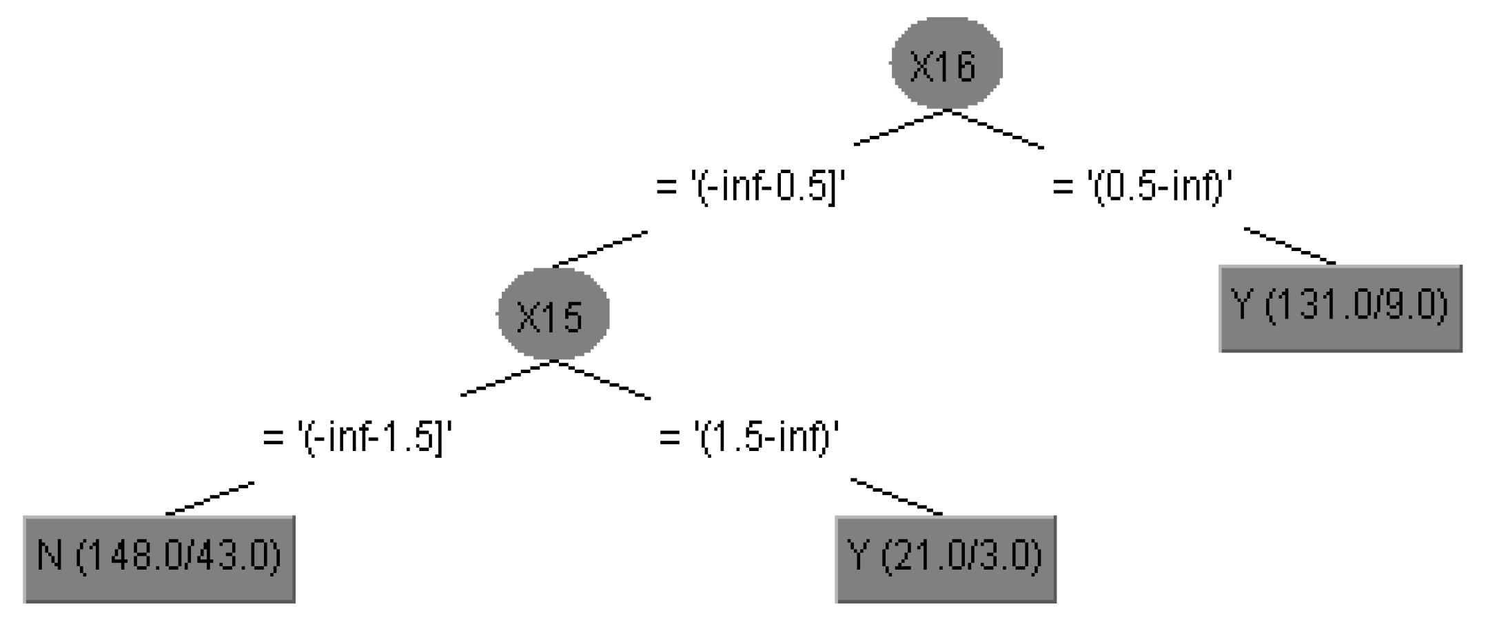
Take whether to repurchase a new insurance policy (X20) as an example. In this study, cross-validation is the evaluation method to generate a decision tree and save calculation time to proactively find the best combination and obtain the knowledge rules and models of the decision tree, which can be used as the model of this study and provide a reference for investors. The decision tree analysis diagram of whether to repurchase a new policy (X20) is shown in Figure 3.

The decision tree analysis diagram is described as follows.

Rule 1: IF X16 > 0.5, THEN X20 = Y. Note: If the time to first purchase is more than 0.5 years (i.e., more than 1 year), the client will repurchase.

Rule 2: IF X16 ≤ 0.5, THEN X15 ≥ 1.5, X20 = Y. Note: If the time to first purchase is less than 0.5 years, and the number of valid policies is more than 1.5 (i.e., two), the client will repurchase a new policy.

Rule 3: IF X16 ≤ 0.5, THEN X15 ≤ 1.5, X20 = N. Note: If the time to first purchase is less than 0.5 years, and the number of valid policies is less than 1.5 (only one), the client will not purchase a new policy.

(2)

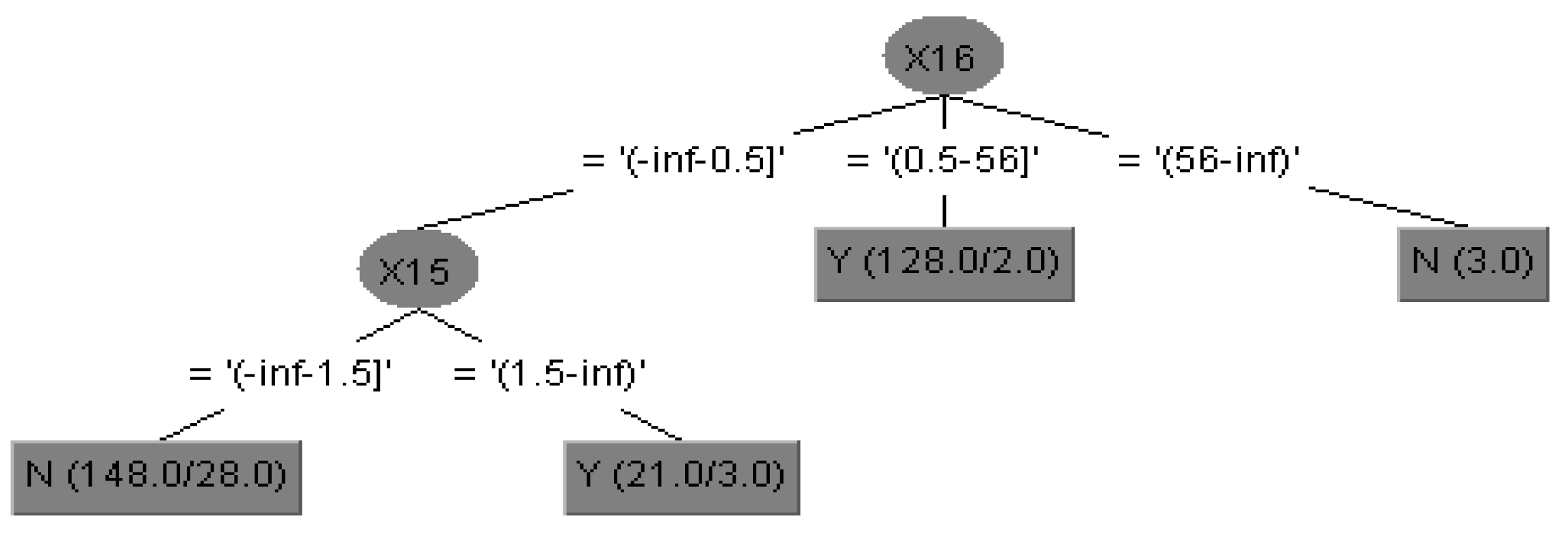
Take whether to introduce new clients (X21) as an example. The decision tree analysis diagram of whether to introduce new clients (X21) generated by the influential important conditional factors is shown in Figure 4.

The decision tree analysis diagram is described as follows.

Rule 1: IF 0.5 > X16 > 56, THEN X21 = Y.

Note: If the time to the first purchase is less than 0.5–56 years (i.e., 1–56 years), the client will introduce new clients.

(3)

Take whether to pay the renewal insurance premium (X22) as an example. The decision tree analysis diagram of whether to pay the renewal insurance premium (X22) generated by the influential important conditional factors is shown in Figure 5.

The Decision Tree analysis diagram is described as follows.

Rule 1: IF X14 < 4.5, THEN X22 = Y.

Note: If the number of policies purchased by the client is less than 4.5, the client will pay the renewal insurance premium.

5. Findings and Management Implications of Empirical Results

In drawing empirical conclusions, the results of this study are obtained and discussed. There are three types of research results, namely research findings, management impacts, and research limitations, which are described as follows.

5.1. Research Findings

The empirical results show that the accuracy of most classifiers notably increased after attribute selection or data discretization, indicating that attribute selection and data discretization are effective. In particular, better results can be obtained when attribute selection and data discretization are used together. From the experimental results, three key points of the research findings for the three classifications of decisional attributes can be addressed and identified as follows.

1.

Whether to repurchase a new insurance policy.

(1)

Disassembly in proportion of whether to repurchase a new insurance policy.

(a)

The best model is Model D with attribute selection and data discretization.

(b)

The best classifier is J48 (maximum accuracy 96.6667%, minimum 88.8889%).

(c)

In Model D, Naïve Bayes increases the most, by 46.6666%.

(d)

The performance of InputMappedClassifier is the worst.

(2)

Cross validation of whether to repurchase a new insurance policy.

(a)

The best model is Model D with attribute selection and data discretization.

(b)

The classifiers with the best accuracy of 83.3333% are J48, K-Star, Bagging, JRip, OneR, PART, and Decision Table.

(c)

In Model I, Naïve Bayes increases the most, by 23.3333%.

(d)

The performance of InputMappedClassifier is the worst.

2.

Whether to introduce new clients.

(1)

Disassembly in proportion of whether to introduce new clients.

(a)

The best model is Model D with attribute selection and data discretization.

(b)

The best classifier is J48 (maximum accuracy 96.6667%, minimum 88.8889%).

(c)

In Model D, Naïve Bayes increases the most, by 46.6666%, and the performance of InputMappedClassifier is the worst.

(d)

The higher the proportion of most classifiers is, the higher the accuracy is, and the smaller the difference of the same classifier is.

(2)

Cross validation of whether to introduce new clients.

(a)

The best model is Model D with attribute selection and data discretization.

(b)

The best accuracy is 89%, with 14 suitable classifiers, including J48.

(c)

In Model I, Naïve Bayes increases the most, by 23.6667%.

(d)

The performance of InputMappedClassifier is the worst.

3.

Whether to pay the renewal insurance premium.

(1)

Disassembly in proportion of whether to pay the renewal insurance premium.

(a)

The best model is Model D with attribute selection and data discretization.

(b)

The best classifier is LMT (maximum accuracy 96.6667%, minimum 89.6926%).

(c)

In Model D, IBK increases the most, by 20%.

(d)

The accuracy of disassembly in proportion in all classifiers is above 70%, and Model D is above 83%.

(2)

Cross validation of whether to pay the renewal insurance premium.

(a)

The best model is Model D with attribute selection and data discretization.

(b)

The best classifier is LMT, with 11 suitable classifiers in total (maximum accuracy 96.6667%, minimum 88.8889%).

(c)

In Model I, IBK increases the most, by 9.6666%.

(d)

The accuracy of all classifiers is above 70%, and Model I is above 85%.

5.2. Managerial Implications

The rapid development of science and technology networks is a technological advantage for enterprises in the real world. The marketing of insurance salespeople should break away from the traditional modes of the past. In the insurance industry, where performance is important, the time and client transaction speed determine income. With this study, we hope to provide insurers and salespeople with practical client development techniques through valuable client insurance policy data, data mining technology, and attribute selection and data discretization technology for analysis, so as to achieve the target of performance growth.

In this study, we adopted the binary classification method for analysis. With this method, the insurers can use existing client data, apply the classification forecasting model to find the hidden client group, and improve the efficiency of new client development modes.

• Whether to repurchase a new policy: In the practice of client management, the transaction takes time, the exploration is time-consuming, and the realistic performance often cannot wait for long-term operation. If we can conduct research and generate rules through technology from the client information, make a list for development, and visit it again, this can save salespeople from having to make fruitless visits to strangers and conducting cold call marketing. Rather, insurers who care about their clients can stimulate their demand and budget and improve the rate of clients who purchase new insurance policies.
• Whether to introduce new clients: In the insurance industry, where service and client relationships are paramount, client sourcing has always been an important issue, and referrals represent the best source of new clients. By the scientific method, data mining can screen for the appropriate referral center and make leveraging effortless, which is important for business development.
• Whether to pay the renewal insurance premium: The client renewal premium is the main focus of the insurer and the insurance salesperson. In this study, we mined client data and used the empirical results to explore the conditional attribute data. These data explore the possible problems of different clients and facilitate client relationship management and adjustment as soon as possible. The topic of client value is often discussed in the industry and in academia. With the steady and sophisticated development of data mining technology, the integration and application of essential data is a major breakthrough for existing clients to engage in redevelopment (including referrals) and to provide reference for insurers and insurance salespeople in client data management.

5.3. Research Limitations

Although the proposed method can achieve satisfactory prediction accuracy in insurance predictions, there are some limitations in the current research. We examined the concerns of the insurance industry regarding the decisions of clients to repurchase new insurance policies, to refer new clients, and to pay renewal premiums. Research data were collected from the insurance industry (a life insurance company in Taiwan). However, due to some limitations, most of the data are basic. Other information involving personal privacy such as the salary, declaration value of the policy, number of family members of the client, and information on policies purchased from other insurance dealers is difficult to obtain. Conditional attributes are not easy to obtain but may affect decision factors. However, based on only 300 data samples in this study, compared with general systems requiring significant training and testing, if more conditional attributes and client data can be obtained, we believe that data analysis in data mining will be more accurate.

6. Conclusions and Future Research

In this study, we predicted the potential target clients using the disassembly in proportion (90/10), cross-validation, and data mining technology for Taiwanese insurance companies only. Based on the results of the empirical analysis, we present the conclusions of this study, research directions that can be pursued in the future, and suggestions.

6.1. Conclusions

We used the data of existing insurance policies through data mining tools to identify the hidden rules and important conditional factors that affect decision attributes and calculate the influence degree to determine the best model and classifier. The results provide suggested rules for policy makers (insurer and insurance salesperson) regarding client data search and compiling lists of target clients.

The empirical results contain the following eight points:

1.

Prediction model: Model A, Model B, Model C, Model D, and Model E. Model D with attribute selection and data discretization performed the best of all the models.

2.

The mixed model is better than the single model in the improvement of evaluation accuracy.

3.

There is little difference in the accuracy between disassembly in proportion and cross-validation.

4.

The better classifiers and the less accurate classifiers were selected by experiments.

(1)

Classifiers with better accuracy (disassembly in proportion): Tree (J48), Bayes (Bayes Net), Function (Simple Logistic), Lazy (LWL), Meta (AdaBoostM1), and Rule (OneR).

(2)

Classifiers with better accuracy (cross-validation): Tree (J48), Bayes (Bayes Net), Function (Simple Logistic), Lazy (LWL and K-Star), Meta (Bagging), Rule (OneR), and Mise (InputMappedClassifier)

(3)

Classifiers with worse accuracy: Naïve Bayes, SMO, SGD Text, Stacking, Vote, ZeroR, and InputMappedClassifier.

5.

According to the binary classification and different decision attributes, there are different important conditional attributes in the empirical analysis influencing the data, and the decision attributes are explained as follows:

(1)

Important conditional attributes and degree of influence of conditional factors regarding whether to repurchase a new insurance policy (X20): gender (X1): 1.0101%; whether the job is in an office (X4): 1.0101%; the amount of long-term care insurance (X13): 3.0303%; the total number of purchased policies (X14): 11.1111%.

(2)

Important conditional attributes and degree of influence of conditional factors regarding whether to introduce new clients (X21): amount of critical illness insurance (X10): 0%; whether there is an investment insurance policy (X11): 6.0606%; number of valid policies (X15): 10.1010%; time to first purchase (X16): 2.0101%; total amount of life insurance including long-term care insurance (X19): 0.0101%.

(3)

Important conditional attributes and degree of influence of conditional factors regarding whether to pay the renewal insurance premium (X22): gender (X1): 1.0101%; family salary structure (X6): 1.0101%; amount of critical illness insurance (X10): 0%; amount of long-term care insurance (X12): −1.0101%; total number of purchased policies (X14): −2.0202%; total premium of personal annual valid insurance policy (X17): 1.0101%; total amount of life insurance including long-term care insurance (X19): 1.0101%; whether to introduce new clients (X21): 0%.

6.

The number of valid policies (X15) and time to first purchase (X6) are the conditional attributes selected by the common attributes of the three decision attributes; the decision attribute of whether to pay the renewal insurance premium (X22) is an important conditional factor, and the two decision attributes influence each other. With the impact of the Silver Tsunami, the government and insurance industry vigorously promote long-term care insurance, and the conditional attributes of amount of long-term care insurance (X12) and premium of long-term care insurance (X13) are the important factors affecting the decision attributes. Regarding the pre-processing of research data, the sequence of attribute selection and data discretization does not affect the accuracy evaluation performance.

7.

Generation of decision tree: The generated rules are easy to understand and can be applied to insurance practices to help salespeople acquire new behavior patterns, make plans that are favorable to clients, and create an ideal situation for clients, companies, and salespeople.

8.

The prediction model also has different performance in different decision attributes. According to the three decision attributes, different classifiers have different performances in the evaluation of disassembly in proportion and cross-verification. The prediction model proposed in this study can be applied to other industries and have different supporting results for different practical problems.

Moreover, the following four directions, including scientific contribution, researchable contribution, managerial contribution, and applicational contribution add to the contributions of this study as follows. (1) Scientific contribution: Although it is not the only or main goal of this study to propose a new methodology for data analysis, determining a suitable hybrid or classifier to identify specific analysis data is important for solving insurance issues from machine learning techniques, since no classifier or model is absolutely suitable for all practical data used in different application domains. Furthermore, the above analytical results offer sound evidence that this study provides a clear contribution for first identifying important uses of key attributes by the attribute selection techniques integrated with the data discretization methods and a variety of data disassemble proportions and the cross-validation method, and the classification technique groups of seven categories to build entropy-based decision rules of knowledge trees for use in insurance applications. Thus, given the above reasons, the study has a significant scientific advantage compared to actuarial literature. (2) Researchable contribution: More importantly, the modeling of such a hybrid system for insurance applications is not seen in other research when compared to past literature reviews; thus, the study has distinct research merit. (3) Managerial contribution: Consequently, our work supports meaningful, entropy-based rules for visualizing tree structures for interested parties and significantly contributes to differentiating classifiers in life insurance data with helpful findings and useful management implications for future research endeavors. These research findings and management implications can contribute useful managerial references used as an alternative approach to mine sustainable life insurance information/knowledge hidden from the study results. (4) Applicational contribution: These novel methods are not the sole objective in the study; conversely, the key applications of these advanced approaches that were emphasized are primarily intensified by the impressive empirical results from challenges of application issues and can benefit from them. This study has a successful case experience and is a good example for life insurance applications.

6.2. Future Research

Although this study has some benefits in predicting the problems of insurance clients, there is still some space for improvement in follow-up research. (1) Insurance dealers can apply data mining technology combined with valuable client policy data on the practice of business promotion, construct a platform to use the rules obtained from data mining, input the list into the system, directly screen the decision attributes (whether to repurchase a new insurance policy, whether to introduce new clients, and whether to pay the renewal insurance premium), and provide the information to the insurance salesperson for quick and accurate client development. (2) The government is concerned with problems such as insufficient average insurance amounts and the promotion of long-term care insurance. In the future, we can continue to study and forecast the products purchased by clients based on the above problems. (3) Future researchers can use different analytical tools for research, such as artificial neural networks (ANNs). (4) Follow-up research can increase the amount of data or increase the conditional data for revalidation. (5) The practical application of the results of this study will be followed up and compared with the results of traditional development and sales to study the difference in effectiveness. (6) For the classifiers with poor accuracy, the reasons and potential improvement could be discussed in future work.

References

- Santos, F.P.; Pacheco, J.M.; Santos, F.C.; Levin, S.A. Dynamics of informal risk sharing in collective index insurance. Nat. Sustain. 2021, 4, 426–432. [Google Scholar] [CrossRef]
- Harris, T.F.; Yelowitz, A.; Courtemanche, C. Did COVID-19 Change Life Insurance Offerings? J. Risk Insur. 2020, 88, 831–861. [Google Scholar] [CrossRef] [PubMed]
- Jimenez-Carvelo, A.M.; Cuadros-Rodríguez, L. Data mining/machine learning methods in foodomics. Curr. Opin. Food Sci. 2020, 37, 76–82. [Google Scholar] [CrossRef]
- Khan, A.; Ghosh, S.K. Student performance analysis and prediction in classroom learning: A review of educational data mining studies. Educ. Inf. Technol. 2010, 26, 205–240. [Google Scholar] [CrossRef]
- Schorn, M.A.; Verhoeven, S.; Ridder, L.; Huber, F.; Acharya, D.D.; Aksenov, A.A.; van der Hooft, J.J. A community resource for paired genomic and metabolomic data mining. Nat. Chem. Biol. 2021, 17, 363–368. [Google Scholar] [CrossRef] [PubMed]
- Ageed, Z.S.; Zeebaree, S.R.M.; Sadeeq, M.M.; Kak, S.F.; Rashid, Z.N.; Salih, A.A.; Abdullah, W.M. A Survey of Data Mining Implementation in Smart City Applications. Qubahan Acad. J. 2021, 1, 91–99. [Google Scholar] [CrossRef]
- Samerei, S.A.; Aghabayk, K.; Mohammadi, A.; Shiwakoti, N. Data mining approach to model bus crash severity in Australia. J. Saf. Res. 2020, 76, 73–82. [Google Scholar] [CrossRef] [PubMed]
- So, B.; Boucher, J.-P.; Valdez, E.A. Cost-Sensitive Multi-Class Adaboost for Understanding Driving Behavior Based on Telematics. ASTIN Bull. 2021, 51, 719–751. [Google Scholar] [CrossRef]
- Guillen, M.; Nielsen, J.P.; Pérez-Marín, A.M.; Elpidorou, V. Can Automobile Insurance Telematics Predict the Risk of Near-Miss Events? North Am. Actuar. J. 2020, 24, 141–152. [Google Scholar] [CrossRef] [Green Version]
- Tiller, J.; Winship, I.; Otlowski, M.F.; Lacaze, P.A. Monitoring the genetic testing and life insurance moratorium in Australia: A national research project. Med. J. Aust. 2021, 214, 157–159. [Google Scholar] [CrossRef]
- Schwegler, U.; Trezzini, B.; Schiffmann, B. Current challenges in disability evaluation and the need for a goal-oriented approach based on the ICF: A qualitative stakeholder analysis in the context of the Swiss accident insurance. Disabil. Rehabil. 2021, 43, 2110–2122. [Google Scholar] [CrossRef] [PubMed]
- George, N.; Grant, R.; James, A.; Mir, N.; Politi, M.C. Burden Associated With Selecting and Using Health Insurance to Manage Care Costs: Results of a Qualitative Study of Nonelderly Cancer Survivors. Med. Care Res. Rev. 2021, 78, 48–56. [Google Scholar] [CrossRef] [PubMed]
- Azzawi, F.J.I.A. Data mining in a credit insurance information system for bank loans risk management in developing countries. Int. J. Bus. Intell. Data Min. 2021, 18, 291–308. [Google Scholar] [CrossRef]
- Choi, S.E.; Simon, L.; Riedy, C.A.; Barrow, J.R. Modeling the Impact of COVID-19 on Dental Insurance Coverage and Utilization. J. Dent. Res. 2020, 100, 50–57. [Google Scholar] [CrossRef] [PubMed]
- Courbage, C.; Nicolas, C. Trust in insurance: The importance of experiences. J. Risk Insur. 2021, 88, 263–291. [Google Scholar] [CrossRef]
- Landais, C.; Spinnewijn, J. The Value of Unemployment Insurance. Rev. Econ. Stud. 2021, 88, 3041–3085. [Google Scholar] [CrossRef]
- Wang, R.; Rejesus, R.M.; Aglasan, S. Warming Temperatures, Yield Risk and Crop Insurance Participation. Eur. Rev. Agric. Econ. 2021, 48, 1109–1131. [Google Scholar] [CrossRef]
- Yun, Y.; Ma, D.; Yang, M. Human–computer interaction-based Decision Support System with Applications in Data Mining. Futur. Gener. Comput. Syst. 2021, 114, 285–289. [Google Scholar] [CrossRef]
- Scheidler, A.A.; Rabe, M. Integral verification and validation for knowledge discovery procedure models. Int. J. Bus. Intell. Data Min. 2021, 18, 73–87. [Google Scholar] [CrossRef]
- Jain, P.K.; Quamer, W.; Pamula, R. Sports result prediction using data mining techniques in comparison with base line model. Opsearch 2021, 58, 54–70. [Google Scholar] [CrossRef]
- Alweshah, M.; Alkhalaileh, S.; Albashish, D.; Mafarja, M.; Bsoul, Q.; Dorgham, O. A hybrid mine blast algorithm for feature selection problems. Soft Comput. 2021, 25, 517–534. [Google Scholar] [CrossRef]
- Cardoso-Ribeiro, F.L.; Matignon, D.; Lefèvre, L. A partitioned finite element method for power-preserving discretization of open systems of conservation laws. IMA J. Math. Control Inf. 2021, 38, 493–533. [Google Scholar] [CrossRef]
- Ahmed, B.; Wang, L. Discretization based framework to improve the recommendation quality. Int. Arab J. Inf. Technol. 2021, 18, 365–371. [Google Scholar] [CrossRef]
- Charbuty, B.; Abdulazeez, A. Classification Based on Decision Tree Algorithm for Machine Learning. J. Appl. Sci. Technol. Trends 2021, 2, 20–28. [Google Scholar] [CrossRef]
- Sahin, E.K.; Colkesen, I. Performance analysis of advanced decision tree-based ensemble learning algorithms for landslide susceptibility mapping. Geocarto Int. 2021, 36, 1253–1275. [Google Scholar] [CrossRef]
- Nandhini, M. Ensemble human movement sequence prediction model with Apriori based Probability Tree Classifier (APTC) and Bagged J48 on Machine learning. J. King Saud Univ. Comput. Inf. Sci. 2021, 33, 408–416. [Google Scholar]
- Mohanty, M.; Subudhi, A.; Mohanty, M.N. Detection of supraventricular tachycardia using decision tree model. Int. J. Comput. Appl. 2021, 65, 378–388. [Google Scholar] [CrossRef]
- Tundo, T. Perbandingan Decision Tree J48, REPTREE, dan Random Tree dalam Menentukan Prediksi Produksi Minyak Kelapa Sawit Menggunakan Fuzzy Tsukamoto. J. Teknol. Inf. Dan Ilmu Komput. 2021, 8, 473–484. [Google Scholar] [CrossRef]
- Abu El-Magd, S.A.; Ali, S.A.; Pham, Q.B. Spatial modeling and susceptibility zonation of landslides using random forest, naïve bayes and K-nearest neighbor in a complicated terrain. Earth Sci. Inform. 2021, 14, 1227–1243. [Google Scholar] [CrossRef]
- Kannan, R.P. Prediction Of Consumer Review Analysis Using Naive Bayes And Bayes Net Algorithms. Turk. J. Comput. Math. Educ. 2021, 12, 1865–1874. [Google Scholar]
- Trangenstein, P.J.; Whitehill, J.M.; Jenkins, M.C.; Jernigan, D.H.; Moreno, M.A. Cannabis Marketing and Problematic Cannabis Use Among Adolescents. J. Stud. Alcohol Drugs 2021, 82, 288–296. [Google Scholar] [CrossRef]
- Comin, H.B.; Sollero, B.P.; Gapar, E.B.; Domingues, R.; Cardoso, F.F. Genome-wide association study of resistance/susceptibility to infectious bovine keratoconjunctivitis in Brazilian Hereford cattle. Anim. Genet. 2021, 52, 881–886. [Google Scholar] [CrossRef] [PubMed]
- Yadav, D.C.; Pal, S. Analysis of Heart Disease Using Parallel and Sequential ensemble Methods with Feature Selection Techniques: Heart Disease Prediction. Int. J. Big Data Anal. Health 2021, 6, 40–56. [Google Scholar] [CrossRef]
- Zarifis, A.; Kawalek, P.; Azadegan, A. Evaluating If Trust and Personal Information Privacy Concerns Are Barriers to Using Health Insurance That Explicitly Utilizes AI. J. Internet Commer. 2021, 20, 66–83. [Google Scholar] [CrossRef]
- Mikucka, M.; Becker, O.A.; Wolf, C. Revisiting marital health protection: Intraindividual health dynamics around transition to legal marriage. J. Marriage Fam. 2021, 83, 1439–1459. [Google Scholar] [CrossRef]
- Marinescu, I.; Skandalis, D. Unemployment Insurance and Job Search Behavior. Q. J. Econ. 2021, 136, 887–931. [Google Scholar] [CrossRef]
- Fang, H.; Kung, E. Why do life insurance policyholders lapse? The roles of income, health, and bequest motive shocks. J. Risk Insur. 2021, 88, 937–970. [Google Scholar] [CrossRef]
- Meagher, T.; Guzman, G.; Heltemes, B.; Senn, A.; Wiseman, S.; Armuss, A.; Wang, Y. Navigating a Pandemic: The Unique Role of the Medical Director. J. Insur. Med. 2021, 49, 11–18. [Google Scholar] [CrossRef] [PubMed]
- Sharma, Y.; Mukherjee, K.; Shrivastav, H. A Study on Factors Impacting the Investment in Life Insurance Policy. Int. J. Manag. Hum. Sci. 2021, 5, 11–15. [Google Scholar] [CrossRef]
- He, A.J.; Qian, J.; Chan, W.-S.; Chou, K.-L. Preferences for private long-term care insurance products in a super-ageing society: A discrete choice experiment in Hong Kong. Soc. Sci. Med. 2020, 270, 113632. [Google Scholar] [CrossRef]
- Martinez-Lacoba, R.; Pardo-Garcia, I.; Escribano-Sotos, F. The reverse mortgage: A tool for funding long-term care and increasing public housing supply in Spain. Neth. J. Hous. Built Environ. 2021, 36, 367–391. [Google Scholar] [CrossRef] [PubMed]
- Terdpaopong, K.; Rickards, R.C. Thai Non-Life Insurance Companies’ Resilience and the Historic 2011 Floods: Some Recommendations for Greater Sustainability. Sustainability 2021, 13, 8890. [Google Scholar] [CrossRef]
- Dash, G.; Chakraborty, D. Digital Transformation of Marketing Strategies during a Pandemic: Evidence from an Emerging Economy during COVID-19. Sustainability 2021, 13, 6735. [Google Scholar] [CrossRef]
- Wolny-Dominiak, A.; Żądło, T. The Measures of Accuracy of Claim Frequency Credibility Predictor. Sustainability 2021, 13, 11959. [Google Scholar] [CrossRef]