Abstract
More countries have made carbon neutral or net zero emission commitments since 2019. Within this context, re-examining the environmental Kuznets curve (EKC) hypothesis plays an essential role in sizing up the global economic development situation and realizing the global carbon emission reduction target. A methodological challenge in testing the EKC hypothesis, which states that increasing income makes CO2 emissions begin to decline beyond a turning point, lies in determining if this benchmark point exists. The EKC hypothesis between income and CO2 emissions is reassessed by applying a new kink regression model for the G7 countries from 1890 to 2015. Results reveal the inverted U-shaped nexus does not exist for US, Germany, Italy, Canada and Japan. For these five countries, the EKC curve has a turning point, but the positive impact of incomes on CO2 emissions becomes significantly smaller after the turning point. We describe this relationship as a pseudo-EKC. K.U.K. and France are the only exceptions, fitting the EKC hypothesis. Further analysis indicates that the relationship between income and SO2 emissions presents an inverted U-shaped curve. Moreover, we observe that the turning point occurs at different points in time for the different G7 countries. Therefore, environmental policies targeting pollutant emission reduction should consider the different characteristics of different pollutants and regions.
1. Introduction
With the global economy set for a growth relapse in recent years, a new round of carbon emission reduction planning has been on the agenda. The environmental Kuznets curve (EKC) debate was engendered by Grossman and Krueger (1991) [1]. It could date back to Kuznets (1955) [2], who put forward an inverted U-shaped relationship between income inequality and economic growth. Grossman and Krueger (1991) [1] proposed an inverted U-shaped path for pollution as a function of income, a frequently employed means for assessing the relationship between economic growth and environmental pollution. Subsequently, a large amount of literature on EKC has emerged [3]. Empirical results are generally mixed. Many studies show the existence of EKC [4]. However, some conclude there is no inverted U-shaped relationship between economic growth and environmental pollution [5].
The EKC hypothesis is important in understanding how to achieve a win–win situation in terms of economic development and enhancing environmental quality [6]. In the past, fossil fuels have contributed to economic growth and national prosperity, but these developments have come at the cost of environmental degradation. The EKC results suggest that economic growth can be compatible with environmental improvements if appropriate policies are adopted and a certain level of technology is achieved [7]. Before adopting policies, it is important to understand the relationship between economic growth and environmental quality [8]. In the current trend of low carbon economic development and environmental governance, the relevant question is: can economic growth play a positive role in achieving carbon emission reductions and improvements in air pollution problems, rather than at the expense of environmental quality? This has been the main motivation for empirical research into EKC [9]. Promoting a low carbon economy, improving the energy mix, and balancing economic growth with carbon reduction goals for sustainable development have received increasing attention from governments and scholars [10]. The results of this study are expected to add to the EKC literature and the literature on carbon mitigation and provide policymakers and practitioners with recommendations on sustainable development to mitigate climate risks and environmental pressures.
Despite a brief decline in carbon emissions within the context of the COVID-19 disease, the United Nations Environment Programme (UNEP)’s Annual Emissions Gap Report 2020 reveals that the world is still on the track, by the end of this century, to warm by more than 3 °C [11]. A growing number of G20 member countries have made carbon neutral or net zero emission commitments since 2019. In this context, re-examining the relationship between economic growth and carbon emissions plays an essential role in sizing up the global economic development situation and realizing the global carbon emission reduction target. As the earliest countries to initiate the industrial revolution, the G7 countries (U.S., UK, France, Germany, Japan, Italy and Canada) have played a great role in promoting and playing an important role in global carbon emission reduction. The G7 countries have rich experience in dealing with environmental challenges, are in a leading position in carbon emission reduction and provide a reference for the design of energy-saving and pollution reduction policies in developing countries. Therefore, it is quite necessary to research the EKC hypothesis between the incomes and CO2 emissions of the G7 countries. The research objectives of this paper are twofold: firstly, have economies such as the G7 countries achieved sustainable development without damaging the environment? In other words, this paper proposes to re-examine the validity of the environmental EKC hypothesis using G7 countries as a sample. Secondly, given the EKC heterogeneity across pollutants and countries [12], this study proposes to examine the manifestation of EKC heterogeneity in the relationship between two pollutants (CO2 and SO2 emissions) and economic growth in different regions (G7 countries), respectively. These results will provide theoretical support and tailor made policy reference for subsequent pollution control and low carbon economic development.
The EKC literature, including both theoretical and empirical studies, is abundant. However, the existence of EKC among G7 countries is still a controversial issue. Therefore, after describing the general concept of the EKC hypothesis, this paper employs a new kink regression model with an unknown threshold proposed by Hansen (2017), to investigate the EKC hypothesis between the incomes and CO2 emissions of the G7 countries [13]. The results show no EKC effect for the nexus for the US, Germany, Italy, Canada, and Japan, with the U.K. and France being exceptions. However, for those that do not fit the EKC hypothesis, the nexus still has a significant turning point; the contribution of incomes to CO2 emissions becomes significantly smaller after the turning point. When income exceeds the threshold, the positive impact of income on CO2 emissions becomes significantly smaller. We observe that the UK, France, Canada, Italy, the US, Germany, and Japan reached their turning points of the EKC curve in about 1972, 1969, 1899, 1891, 1912, 1914 and 1972. We describe this relationship as a pseudo-EKC and attempt to explain this phenomenon using the concept of the free-rider problem.
This study makes important contributions to the bulk of literature based on the scope of analysis and the econometric methodology employed. First, evidence of EKC is usually based on time series data that spans a period during which there is evidence of gains in environmental quality [14]. Previous literature focusing on relatively small datasets, spanning only a few decades, does not provide an effective way to directly estimate and test for the presence of an unknown turning point of income. We examine the EKC hypothesis of the G7 countries using a larger dataset that spans nearly 150 years. Second, we employ a new kink regression model with an unknown threshold. Consistent with a large set of theoretical models, this model can estimate and examine the existence of EKC and the presence of the unknown threshold value of income. It can test whether there exists an unknown threshold effect on carbon emissions and directly reveal the turning points of EKC. Third, we provide evidence that there are pseudo-EKC nexuses between incomes and CO2 emissions for the five G7 countries.
The rest of our study is structured as follows. The relevant literature on the EKC hypothesis is discussed in Section 2. The methodology and data used in this study are described in the subsequent section. Section 4 presents the empirical findings and robustness analysis. In Section 5, the discussion and conclusions are provided.
2. Literature Review
2.1. Theoretical Explanations Supporting the EKC Hypothesis
Many scholars have made a detailed theoretical explanation of the formation of the traditional EKC theory, mainly from five perspectives: economic structure change, income inequality and demand preference, international trade, technological progress and policy guidance [9]. Shafic and Bandyopadhyay (1992) [15] point out that economic structure change, also known as industrial restructuring, is important for environmental quality. This refers to the adjustment from the development stage based on traditional energy intensive and heavy industry to the economic stage based on a technology intensive, information technology, and service industry [15]. In the first stage of development, the level of the byproducts of output, i.e., pollution, rises gradually with economic expansion, and economic growth is positively correlated with environmental pollution [16]. With the upgrading and restructuring of the industry structure, information technology industries and services would no longer bring more pollution and would, therefore, bring opportunities for environmental improvement, thus shifting the EKC curve to the second stage of negative correlation [7].
The second motivation for the EKC curve is income inequality and changes in demand preferences. With the improvement in the national income level, the population’s income distribution would become more equitable [9]. An increase in residents’ incomes will raise their preferences for environmental quality and increase people’s awareness of environmental protection and spending on environmental protection research [17]. In addition, residents may pressure governments to implement stricter environmental regulations through activities such as marches and elections [18].
The third explanation comes from international trade. Countries use their comparative advantages to trade with each other. For this reason, developed countries are engaged in high technology industries, while developing countries are engaged in industries characterized by labor intensive industries and high pollution, for economic growth [19]. Developed countries tend to be more stringent in terms of environmental regulations, so these countries choose to move industries with high pollution to developing countries that pay less attention to environmental regulations. This transfer of polluting industries leads developed countries to the declining stage of the EKC curve [20].
Besides, the technological progress effect can also play an important role in the EKC curve. It consists of two aspects: first, technological progress increases productivity, such as improved energy efficiency. Namely, the same economic growth can be achieved by investing fewer resources. Second, the investment in clean technologies, such as new energy sources, leads to the gradual greening of production processes, thus combating the environmental pollution problem at the source [21,22]. Last but not least, when economic development reaches a certain high level, the government and people start to pay attention to the environmental pollution problem and take measures to protect the environment. By adopting market mechanisms, such as carbon trading mechanisms, sulfur trading mechanisms, carbon taxation and other price instruments [23], consumers and producers are motivated to pay attention to controlling environmental pollution and improving energy use and production efficiency [24]. Accordingly, some scholars argue that the downward phase of the EKC curve is not a result of increasing income but the government’s initiative and policy guidance [25].
In general, the above studies have highlighted the importance of adding various influencing factors to study of the EKC hypothesis, such as income inequality, technological progress, and government regulation. These factor studies provide the basis for empirical research on EKC and thus better avoid omitted variables. However, a large number of empirical studies also find that the EKC hypothesis does not exist, and the theoretical explanation for this category of findings is still inadequate, by comparison.
2.2. Development and Debate of EKC Theory in Recent Years
In recent years, empirical research on EKC has remained a hot issue. Although many scholars have studied the EKC hypothesis, its research results have contradictory conclusions. Firstly, the relationship between economic growth and environmental degradation is highly sensitive to the choice of functional form and estimation method [26,27,28]. For example, in developed versus developing countries, importance should be attached to the distinction between the choice of a quadratic or cubic model of GDP per capita [17], since the explanatory power of the economic growth polynomial accounts for a much smaller proportion of the environmental improvement species in developed countries than in low and middle income countries [28,29]. Secondly, the variety in conclusions could come from the problem of omitted variables in the model [30]. Existing literature finds that the environmental impact per unit of economic activity is affected by income distribution [17,18], government regulation [23,24,25], scientific and technological progress [30,31], energy consumption [32,33,34] and many other factors. Thirdly, there are differences in selecting country samples and periods for various studies [17,35,36]. Until the early 2000s, most studies used cross-sectional data that included only one country [37]. The time dimension lacks long overlapping observations among panel data studies [38]. Therefore, it is important to extend the period to increase the overlap between countries [38,39]. This is particularly vital for analyses of carbon emissions, which originate from changes in energy use and should, therefore, be analyzed more from a long term perspective [40].
Concerning air pollution, one of the most representative EKC research objects, the academic debate about whether the relationship between air pollution and economic growth has a similar evolutionary law did not get a consistent conclusion. Table 1 summarizes some studies on EKC. Specifically, a classical inverted U-shaped relationship is represented by Grossman and Krugger (1991) [7], which confirms an inverted U-shaped curve relationship between per capita income and SO2 pollution levels through the GLS method. In addition, a large number of empirical experiences support this conclusion from other country samples [30,31]. In addition to taking a cross country panel data sample, using a single country with provincial and municipal level panel data samples, Rafindadi (2016) [41] and Chang et al. (2021) [42] found that different regions in the same country, with differences in economic development levels, also have significant environmental Kuznets curve effects. However, Holtz-Eakin and Selden (1995) [43] found a positive relationship between economic growth and environmental pollution. Friedl and Getzner (2003) [44] and Shao et al. (2016) [45] found that economic growth and environmental pollution do not have an inverted U-shape, but rather an N-shape and U-shape. Besides, Baek (2015) [46] and Park and Lee (2011) [47] suggest there is no significant EKC relationship between environmental pollution and economic growth.

Table 1.
Typical literature related to the EKC hypothesis.
In addition, there are also widespread disputes on the choice of models. Most current research regarding the EKC hypothesis uses a classical reduced form approach and linear econometric models, including primary, quadratic, and cubic linear models, resulting in multicollinearity problems [53]. With the development of methods and the improvement in data in recent years, more and more new methods are used to evaluate EKC theory, such as the fixed effect regression model with Driscoll–Kraay standard errors and the common correlated effects mean group (CCEMG) estimator [54]; the error correction based panel autoregressive distributed lag (ARDL) model augmented with cross-sectional averages [55]; and the moments quantile regression approach [56]. Particularly, a minority of the literature, such as Churchill et al. (2020) [49], avoids the issue of model form and uses nonparametric methods to test the EKC hypothesis. The use of panel data in EKC empirical studies assumes that the overall sample fits the EKC pattern, but not every country follows this pattern individually [22]. An individual country’s turning points may differ significantly from those estimated for the overall sample. Therefore, empirical EKC studies should focus on each country separately [57,58,59] or use longer time series data [38,39].
Overall, there are many explanations for the reasons for EKC. From the above analysis of the causes of the EKC hypothesis, it is clear that, when there are large differences in income levels, economic development structures, national policies, international trade and scientific and technological progress, the EKC curves of different countries present different shapes. The relationship between environmental pollution and economic growth may exhibit forms other than the inverted U-shape, such as the U-shape and N-shape. The timing of the turning points will also be different with country and regional characteristics. Current studies have reached inconsistent conclusions about the EKC hypothesis. Therefore, it cannot be generalized to all pollutants and countries. In other words, it is not universally applicable. Collectively, the understanding of the EKC hypothesis is largely based on a number of empirical studies based on samples from countries around the world and over various periods. However, in those studies that do not conform to the inverted U-shaped performance of the EKC, there are relatively few theoretical explanations for the income–pollution relationship and why the EKC concept is no longer valid.
Considering that the inconsistency between all this evidence comes from different samples, Churchill et al. (2018) [38] and Shahbaz and Sinha (2019) [39] point to the importance of extending the period to increase the overlap between countries. This paper uses a long-time sample, from 1870–2015, to avoid misleading results. In addition, most previous studies have utilized classical linear econometric models to assess the EKC hypothesis. This paper used a threshold effects regression model proposed by Hansen (2017) [13] to analyze the EKC problem, which allows for a more precise grasp of the timing of the emergence of the turning point. Meanwhile, based on the finding that some countries do not conform to the EKC hypothesis, this paper attempts to further explain this phenomenon through the free-rider theory [60].
3. Methodology and Data
3.1. Methodology
EKC hypothesis argued that pollution tends to slow when income level exceeds a threshold. We employ a kink regression model with an unknown threshold to examine whether the G7 countries fit the EKC hypothesis. The regression kink model is a modification of the regression discontinuity model. The traditional regression discontinuity model assumes that the threshold is known, but it is unknown and must be estimated in some cases. This kink regression model with an unknown threshold was first proposed by Hansen (2017) [13], and can explain a nonlinear relationship between each independent variable and the dependent variable by threshold estimation. This model’s function is continuous, but its slope discontinues at the kink or turning point. This model can be applied in a single time series that has the advantage of not imposing homogeneity. Meanwhile, this model extends the regression discontinuity model [61]. It is continuous but with a slope that produces a “kink” at the threshold. Hansen (2017) [13] used this model to study the nonlinear relationship between debt and economic growth based on long span time-series data from the United States of America. Since it is not known where the turning point of the relationship between economic growth and environmental quality will occur, this model allows us to estimate the model without knowing the specific threshold by the discontinuity, which provides a “kink” in its continuous regression function. Besides, this model can directly capture the nonlinear relationship between economic growth and environmental quality without converting the data into quadratic form, as is commonly performed in previous works. Maneejuk et al. (2020) [62] argued that estimating quadratic functions is associated with overly distorted data. In addition, the quadratic term model is accompanied by the problem of multicollinearity between the primary and secondary terms of GDP. The estimation results may not be well constructed for the relationship between economic growth and environmental quality [53]. Moreover, using this model proposed by Hansen (2017) [13] to examine the presence of EKC in the context of individual countries and each group of countries, enables us to examine the heterogeneity of the EKC effect, explore the threshold effect of economic growth on environmental improvement, and capture the jump characteristics of different developing countries in this relationship [63]. Many existing papers, such as Kaika and Zervas (2013) [59] and Al-Mulali et al. (2016) [53], have criticized the classical quadratic term models and econometric models used in studies on empirical EKC from the above literature review. There is no evidence that all countries follow a common inverted U-shaped environmental–economic relationship in their economic growth process, because this relationship can be affected by various factors, such as national income, technological progress, and severity of environmental regulations in different countries [9].
Generally, under this framework, the EKC hypothesis test for G7 countries can be formalized as a regression kink model, where the log per capita emissions is the dependent variable, and the log per capita GDP is the key regressor and threshold variable. If we estimate the threshold point of income and prove that when the income for a country exceeds the threshold then the estimated coefficients of the income–CO2 emissions are negative, but it is positive before the threshold, it means this satisfies EKC hypothesis.
Based on the kink regression model with an unknown threshold, the EKC regression test model is [13]:
where denotes the log per capita CO2 emissions or SO2 emissions, and denotes the log per capita GDP for every G7 countries, ; is the disturbance. Function and denote the “negative part” and “positive part” of , respectively; where is a cut off level of , called the “threshold”, is the intercept. The slope with respect to the variable equals for log per capita GDP less than ; and the slope with respect to the variable equals for log per capita GDP more than . In this paper, is rejected, and meanwhile if , we claim that the EKC hypothesis is confirmed.
3.2. Variable
In this paper, we choose CO2 emissions to measure environmental quality. EKC theory refers to the relationship between economic development and the degree of environmental pollution in a country. Antle and Heidebrink (1995) [64] pointed out that the concept of environmental quality has a broad conceptual and multidimensional nature. Environmental problems include air and water pollution and the growing issue of global warming, which is still the greatest global risk in 2022 according to the WEF’s Global Risks Report 2022 [65]. The main contributor to greenhouse gas emissions and the gas that stays in the atmosphere the longest is CO2 [31], and CO2 emissions are also an indicator of air pollution [66]. As CO2 emissions is a special case of environmental degradation with global effects [59], many studies have explored the EKC relationship between CO2 emissions and economic growth, using greenhouse gas emissions as an indicator of environmental pollution [27,28,43,44,67,68,69]. Environmental stresses, such as extreme disasters caused by climate change, are increasing, directly linking carbon emissions and environmental degradation. This is why we choose CO2 emissions as the measurement of environmental quality.
3.3. Data
Industrialization emerged around 1870, and we use 1870 as the starting point for our analysis. The data consist of annual information on per capita CO2 emissions taken from the Carbon Dioxide Information Analysis Center, which provides us with a total sample size of 1050 observations consisting of 7 countries over the period 1870–2015 (Japan is 1950–2015 due to incomplete data); real GDP per capita data in constant USD, the base year 1985 were obtained from the Historical Statistics of the World Economy from 1870 to 2015 [70]. All the series are transformed into logs (natural logarithm) before empirical analysis.
Summary statistics of the variables are revealed in Table 2. Note that, during 1870–2015, the United States had the highest average per capita GDP, with a standard deviation of 0.7985. Italy’s average per capita GDP is lowest, with the largest standard deviation, which is the largest standard deviation among G7, indicating that the Italian economy has great volatility. Regarding the per capita CO2, the U.S. has the highest emissions among G7. Besides, note that the per capita CO2 emissions for G7 are skewed to the left, and the real GDP per capita for G7 skewed to the right, with all the variables having excess kurtosis. The Jarque–Bera test overwhelmingly rejects the null of normality. This evidence of fat tails in the variables provides us with the preliminary motivation to use a nonlinear regression model rather than a standard linear regressions model based on the conditional mean.
Table 2.
Summary statistics results.
We perform standard unit root tests to determine whether the series is stationary, since the kink regression model with an unknown threshold used in this paper assumed the variables have no unit root. Test results are reported in Table 3. According to results in Table 3, the augmented Dickey and Fuller (ADF) test by Dickey and Fuller (1979) [71] and the Phillips–Perron (P.P.) test by Phillips and Perron (1988) [72] reject the null hypothesis of nonstationarity for some series, but it cannot work for most. This result may be because ADF and P.P. tests have a major shortcoming in that they do not allow for the possibility of structural breaks. Therefore, we use the Zivot-Andrews unit root test proposed by Zivot-Andrews (1992) [73], which allows a break at an unknown location both on the trend and intercept for all variables. The results of the Zivot-Andrews unit root test and the estimated break date are also shown in Table 3. The Zivot-Andrews unit root test confirms that these series are stationary. There is a break for all countries’ per capita CO2 emissions and real GDP per capita. This finding of breakpoints in the variables indicates that the linear model based on mean estimation is not suitable to depict the relationship between them. Perhaps it is a nonlinear link.
Table 3.
Unit root test results.
4. The Empirical Findings
4.1. Main Findings of CO2 Emission
Table 4 and Figure 1 display the estimated results between log per capita GDP and log per capita CO2 emissions for the G7 countries. There is no inverted U-shaped nexus between the income per capita and CO2 emissions for the US, Germany, Italy, Canada, and Japan, except for the U.K. and France. Nevertheless, we find that income has a threshold effect for these countries that does not fit the traditional EKC hypothesis. When income exceeds this threshold, the estimated coefficients of the income–CO2 emissions are positive but significantly smaller than before the threshold. Taking the U.S as an example, the F-test indicates the presence of a threshold at the 1% significance level. We also provide the R-squared as the goodness of fit for each regression, proving that each model is good. The estimated threshold value is 8.56. When GDP per capita is less than 8.56 (the low-income period), the regression coefficient of CO2 emissions is 2.25 and is significant at the 5% level. When the income exceeds this threshold (the high-income period), the regression coefficient is 0.18, still greater than zero, but less than . This implies that the positive impact of income on CO2 emissions becomes much smaller with income increase. Economic growth and CO2 emissions are positively correlated, but the marginal propensity to emit carbon dioxide decreases as GDP per capita increases. This finding is in line with Holtz-Eakin and Selden (1995) [43]. We define this relationship as the pseudo-EKC, and we suggest that a major factor causing this phenomenon is the free-rider problem [60]. Shafik (1994) [27], Galeotti and Lanza (2005) [74] and Aslanidis and Iranzo (2009) [75] also verified that the main explanation we may find is related to the free-rider problem. Shafik (1994) [27] and Aslanidis and Iranzo (2009) [75] believe that, because other regions bear all the costs of climate change, and, in most cases, the local benefits are very small in the short term, there is no significant cost of CO2 emission locally. The free-rider problem is an economic phenomenon identified by Olson (2009) [76]. This issue arises in response to the world’s public goods, which are characterized by their shared nature. Ethical standards require people to contribute to the use and maintenance of public goods. We propose the following mechanisms to explain this problem. Based on the perspective of supply and demand, the publicity of environmental protection related affairs may lead to insufficient supply of environmental protection commodities, which may further lead to market failure. This phenomenon is caused by the local government’s “free-rider” problem, when the governments of neighboring countries strengthen environmental protection [77]. Besides, the transboundary nature of the air may encourage free-riding. Given the opportunity costs that could have been used to improve other economic indicators in the region, regional administrations and individuals lose the motivation to control their air pollution, which will lead most regions and individuals to take inaction and only wait for neighbors to take actions, making the “free-rider” problem more serious [78]. Last, in the context of global warming, the lack of incentives to internalize the negative effects of local economic activities is particularly strong. The public nature of global warming means that, once emissions are reduced, every country and everyone can equally enjoy the benefits of greenhouse gas emission reduction. Therefore, it is reasonable from a personal point of view to hitch a “free-rider” on the control projects being implemented in other countries [79].
Table 4.
Kink regression with the unknown threshold for CO2 emissions.
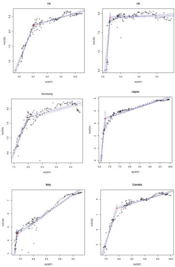
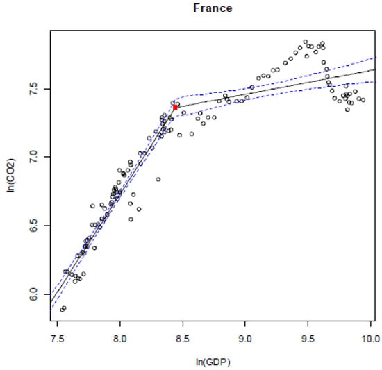
Figure 1.
Scatter plot of real GDP and CO2 emissions, with estimated kink regression model, and 95% confidence intervals. The dots show the pairs of observations of and . The red dot is the estimated threshold.
The issue of carbon reduction and combating climate change is a public good that all countries need to maintain. However, as long as one person contributes to maintaining the public good, others can enjoy the creation of that public good. At the same time, they quietly wait for others to contribute, thus achieving free-riding and unearned benefits. However, due to the goal of economic growth and rational considerations, there may be a strong tendency for countries to adopt a free-rider strategy, hoping that they can rely on others to complete the task of reducing carbon emissions. A Kuznets inverted U effect for U.K. and France is in line with Wagner (2015) [80]. For the other five countries that do not fit the EKC hypothesis, our US, Canada, and Italy results are similar to Onater-Isberk (2016) [81]. Our results for Germany and Japan are similar to Jaunky (2011) [50]. However, our result is different from the idea of some former research, which provided support for the EKC hypothesis in G7 countries [82,83]. Meanwhile, Chang (2015) [84] found that the G7 countries did not satisfy the environmental Kuznets curve hypothesis, but our point disagrees with the previous study results offered by Chang (2015) [84].
In contrast to models that indirectly get the turning points of the EKC curve, the threshold value directly identifies the historical time of the G7 countries’ turning points on the EKC curve. Turning points in the U.K. and France approximately go back to 1972 and 1969, respectively, when CO2 emissions declined rapidly with income growth. However, for Canada and Italy, their turning points are approximately 1899 and 1891, respectively. The turning point for US, Germany and Japan is later, approximately 1912, 1914 and 1972, respectively, and the effect of income on CO2 emissions is still positive but smaller. The time difference of the turning point of the EKC curve in the G7 countries mainly results from their respective economic scale effect, population size effect, economic structure effect, technical progress effect, international trade effect and policy effect. Therefore, the specific situation of their turning point is completely different.
4.2. Robust Analysis about SO2 Emission
To further verify, compare and check the robustness of the analysis, we now turn to SO2 pollution. Meanwhile, for verifying that the sample periods have no impact on our study results, we select the SO2 data of G7 countries over time from 1870 to 2001. We also carry on the unit root tests for the time series of SO2 for G7 countries using the Zivot-Andrews unit root test. The results indicate that these series are stationary and fill the modelling conditions (see Table 3). Table 5 and Figure 2 display the estimated results between log per capita GDP and log per capita SO2 emissions for the G7 countries. The F-test indicates the presence of a threshold at the 1% significance level. The regression coefficient of SO2 emissions for all the G7 countries is positive, and the regression coefficient of SO2 emissions for all the G7 countries is negative, which means the EKC hypothesis is confirmed. Our empirical results show that the EKC hypothesis is perfectly valid in G7 for the nexus between incomes and SO2 emissions, which is in line with the classical literature [10,51,80,85]. These papers focused on the relationship between income and SO2 emissions, and all identified an inverted U-shaped relationship in G7. However, our results are different than the study results offered by Park and Lee (2011) [47], who find that there is no identical shape of EKC for SO2 emission in different regions.
Table 5.
Kink regression with the unknown threshold for SO2 emissions.
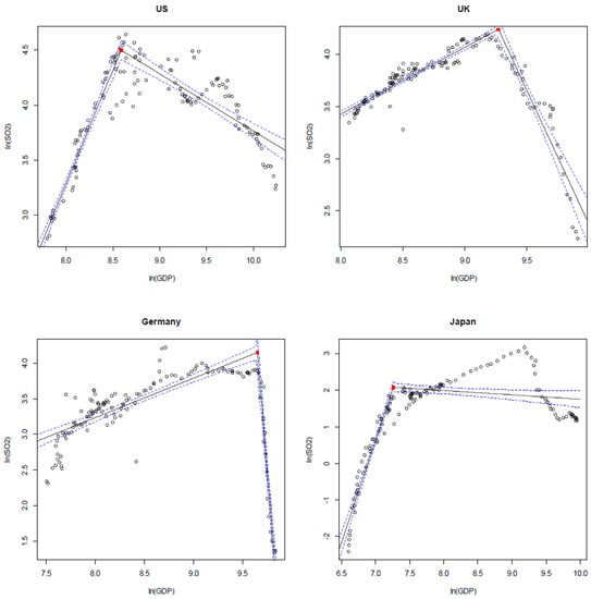
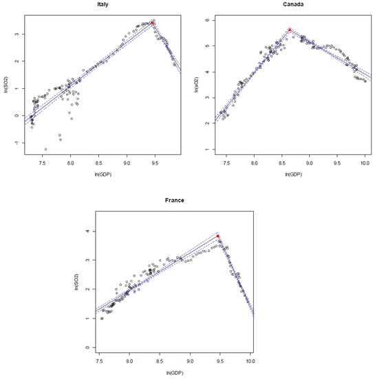
Figure 2.
Scatter plot of real GDP and SO2 emissions, with estimated regression kink model, and 95% confidence intervals. The dots show the pairs of observations of and . The red dot is the estimated threshold.
In summary, CO2 emissions and SO2 emissions have different relationships with income, possibly due to the following two reasons. On the one hand, the source range of CO2 emissions is wider than SO2 emissions. CO2 emissions are produced in the industrial production activities and stem from the ordinary lives of residents. By comparison, the SO2 emission source range is relatively narrow. On the other hand, with the growth in the economy and the improvement in income, the consumption of energy structure has been changing. Even in the same country, there is no single dominant shape of the EKC curves for the various pollutant, namely, SO2 and CO2. Further analysis of SO2 emissions implies that environmental policies targeting pollutant emissions reduction should consider the different characteristics of different pollutants and regions.
5. Discussion and Conclusions
5.1. Conclusions
This paper re-examines the EKC hypothesis in the G7 countries based on CO2 and SO2 emissions data by employing a new kink regression model with an unknown threshold. The results show no inverted U-shaped nexus between the income per capita and CO2 emissions for the US, Germany, Italy, Canada and Japan, except for U.K. and France. Nevertheless, we find that income has a threshold effect for these countries that not does fit the EKC hypothesis. We call this relationship a pseudo-EKC. The turning point of the EKC curve is evident for the UK, France, Canada, Italy, US, Germany and Japan, and occurs in 1972, 1969, 1899, 1891, 1912, 1914 and 1972, respectively. In addition, this paper finds that the relationship between CO2 and economic growth is a “pseudo” EKC, while SO2 exhibits an inverted U-shape, consistent with the EKC curve hypothesis. Therefore, the EKC hypothesis cannot be generalized to all pollutants and all countries.
5.2. Discussions and Policy Implications
According to the research conclusions, this paper puts forward the following policy suggestions: First, since the stage of negative correlation between economic growth for carbon emission reduction has not yet been reached in most countries, the government must take care to avoid contradictions between policies to control greenhouse gas emissions and economic development policies in the future [43]. Therefore, policymakers must strategically design and implement interventions to promote economic growth, improve environmental quality and promote sustainable development. For example, in the long run, for economic and environmental benefits, compatible green economic growth policies such as carbon pricing and increasing subsidies for green energy activities should be encouraged. Second, environmental policies need to be customized for each pollutant, rather than being standardized measures. In other words, governments should formulate relevant policies and take different measures to reduce air pollution according to the EKC characteristics of different air pollutants. Third, each country should formulate corresponding policy objectives according to the time of the turning point. As sustainable development is crucial to every G7 country, environmental pollution is an important obstacle to national sustainable development. Therefore, to reduce environmental pollution, we must raise public awareness and carry out necessary structural reform to make per capita GDP reach a turning point.
There are some limitations of our study in this paper, such as the data collection, analysis and interpretation that the modelling should further support. Meanwhile, many areas of the investigation remain for future studies. For example, we should further develop a framework to further analyze the reasons for the turning point of pollutant emissions in G7 countries at a certain historical point, which can help policymakers identify the correct mechanism to drive national carbon emission reduction. Second, we still need to build a model to further analyze why the evidence from SO2 data indicates the existence of EKC, but the evidence from CO2 data indicates that it does not exist. Third, the explanation of the free-rider effect in the main results proves the complexity of carbon emissions reductions across countries. It suggests that solving the problem of collective global action by a country and its government alone is inherently unworkable [86,87,88]. Therefore, effectively reducing the occurrence of the “free-rider” as much as possible is an important problem to be discussed in the future. Fourth, our current study does not analyze the heterogeneity of different G7 countries. Future research needs to increase comparative regional analysis to find the impact of carbon emissions in different countries and other economic conditions. In particular, to better understand environmental sustainability, future research can use other greenhouse gases, such as methane and nitrous oxide.
Author Contributions
Conceptualization, P.-Z.L., Y.-S.R. and Y.J.; methodology, P.-Z.L. and Y.J.; software, P.-Z.L. and Y.-S.R.; validation, P.-Z.L., Y.-S.R. and Y.J.; formal analysis, P.-Z.L., Y.-S.R. and Y.J.; investigation, Y.-S.R. and Y.J.; resources, Y.-S.R. and Y.J.; data curation, P.-Z.L. and Y.J.; writing—original draft preparation, P.-Z.L., Y.-S.R. and Y.J.; writing—review and editing, S.N., K.B. and B.S.; visualization, Y.J. and Y.-S.R.; supervision, Y.J., Y.-S.R., S.N., K.B. and B.S.; project administration, Y.-S.R. and Y.J.; funding acquisition, Y.-S.R. and Y.J. All authors have read and agreed to the published version of the manuscript.
Funding
This research was funded by the National Natural Science Foundation of China, grant number 72104075; 72101120; 71850012, the National Office for Philosophy and Social Sciences Fund of China, grant number 19AZD014, the Hunan social science achievement review committee, grant number XSP21YBC087, Youth project of Jiangsu Social Science Foundation, grant number 21EYC001, The third phase of Applied Economics of Nanjing Audit University for advantageous disciplines in Colleges and universities in Jiangsu Province project, grant number [2014]37, and the Hunan University Youth Talent Program.
Institutional Review Board Statement
Not applicable.
Informed Consent Statement
Not applicable.
Data Availability Statement
Data will be available on request.
Acknowledgments
The authors would like to thank Hunan University for sponsoring this research. Meanwhile, the authors would like to thank the editor and anonymous reviewers for their patience and helpful comments on the earlier versions of this paper.
Conflicts of Interest
The authors declare no conflict of interest.
References
- Grossman, G.M.; Krueger, A.B. Economic growth and the environment. Q. J. Econ. 1995, 110, 353–377. [Google Scholar] [CrossRef] [Green Version]
- Kuznets, S. Economic Growth and Income Inequality. Am. Econ. Rev. 1955, 45, 1–28. [Google Scholar]
- Özokcu, S.; Özdemir, Ö. Economic growth, energy, and environmental Kuznets curve. Renew. Sustain. Energy Rev. 2017, 72, 639–647. [Google Scholar] [CrossRef]
- Jalil, A.; Feridun, M. The impact of growth, energy and financial development on the environment in China: A cointegration analysis. Energy Econ. 2011, 33, 284–291. [Google Scholar] [CrossRef]
- Martinez-Zarzoso, I.; Bengochea-Morancho, A. Pooled mean group estimation of an Environmental Kuznets Curve for CO2. Econ. Lett. 2004, 82, 121–126. [Google Scholar] [CrossRef]
- Sarkodie, S.A.; Strezov, V. Empirical study of the Environmental Kuznets curve and Environmental Sustainability curve hypothesis for Australia, China, Ghana and USA. J. Clean. Prod. 2018, 201, 98–110. [Google Scholar] [CrossRef]
- Grossman, G.M.; Krueger, A.B. Environmental Impacts of a North American Free Trade Agreement; National Bureau of Economic Research: Cambridge, MA, USA, 1991. [Google Scholar]
- Coondoo, D.; Dinda, S. Causality between income and emission: A country group-specific econometric analysis. Ecol. Econ. 2002, 40, 351–367. [Google Scholar] [CrossRef]
- Kaika, D.; Zervas, E. The Environmental Kuznets Curve (EKC) theory—Part A: Concept, causes and the CO2 emissions case. Energy Policy 2013, 62, 1392–1402. [Google Scholar] [CrossRef]
- Nieto, J.; Carpintero, Ó.; Miguel, L.J.; de Blas, I. Macroeconomic modelling under energy constraints: Global low carbon transition scenarios. Energy Policy 2020, 137, 111090. [Google Scholar] [CrossRef] [Green Version]
- UNEP. Emissions Gap Report 2020; U.N. Environment Programme: Nairobi, Kenya, 2020. [Google Scholar]
- He, L.; Zhang, X.; Yan, Y. Heterogeneity of the Environmental Kuznets Curve across Chinese cities: How to dance with ‘shackles’? Ecol. Indic. 2021, 130, 108128. [Google Scholar] [CrossRef]
- Hansen, B.E. Regression Kink with an Unknown Threshold. J. Bus. Econ. Stat. 2017, 35, 228–240. [Google Scholar] [CrossRef]
- Chimeli, A.B. Growth and the environment: Are we looking at the right data? Econ. Lett. 2007, 96, 89–96. [Google Scholar] [CrossRef]
- Shafic, N.; Bandyopadhyay, S. Economic Growth and Environmental Quality. Time-Series and Cross Country Evidence. Policy Research Working Paper No. 904; World Development Report 1992; The World Bank: Washington, DC, USA, 1992. [Google Scholar]
- Panayotou, T. Economic Growth and the Environment 2003. Economic Survey of Europe; UNECE: Geneva, Switzerland, 2003; Volume 2, Chapter 2. [Google Scholar]
- Magnani, E. The Environmental Kuznets Curve, environmental protection policy and income distribution. Ecol. Econ. 2000, 32, 431–443. [Google Scholar] [CrossRef]
- Khanna, N. The income elasticity of non-point source air pollutants: Revisiting the environmental Kuznets curve. Econ. Lett. 2002, 77, 387–392. [Google Scholar] [CrossRef]
- López, R. The Environment as a Factor of Production: The Effects of Economic Growth and Trade Liberalization. J. Environ. Econ. Manag. 1994, 27, 163–184. [Google Scholar] [CrossRef]
- Suri, V.; Chapman, D. Economic growth, trade and energy: Implications for the environmental Kuznets curve. Ecol. Econ. 1998, 25, 195–208. [Google Scholar] [CrossRef]
- Selden, T.M.; Song, D. Environmental quality and development: Is there a Kuznets curve for air pollution emissions? J. Environ. Econ. Manag. 1994, 27, 147–162. [Google Scholar] [CrossRef]
- De Bruyn, S.M.; van den Bergh, J.C.J.M.; Opschoor, J.B. Economic growth and emissions: Reconsidering the empirical basis of Environmental Kuznets Curves. Ecol. Econ. 1998, 25, 161–175. [Google Scholar] [CrossRef]
- Wara, M. Is the global carbon market working? Nature 2007, 445, 595–596. [Google Scholar] [CrossRef]
- Fan, Y.; Wu, J.; Xia, Y.; Liu, J.-Y. How will a nationwide carbon market affect regional economies and efficiency of CO2 emission reduction in China? China Econ. Rev. 2016, 38, 151–166. [Google Scholar] [CrossRef]
- Panayotou, T. Demystifying the environmental Kuznets curve: Turning a black box into a policy tool. Environ. Dev. Econ. 1997, 2, 465–484. [Google Scholar] [CrossRef] [Green Version]
- Grossman, G.M.; Krueger, A.B. Environment Impacts of a North American Free Trade Agreement. In The Mexican-US Free Trade Agreement; Garber, P.M., Ed.; MIT Press: Cambridge, UK, 1993; pp. 1–10. [Google Scholar]
- Shafik, N. Economic Development and Environmental Quality: An Econometric Analysis. Oxf. Econ. Pap. 1994, 46, 757–773. [Google Scholar] [CrossRef]
- Roberts, J.T.; Grimes, P.E. Carbon intensity and economic development 1962–1991. A brief exploration of the environmental Kuznets curve. World Dev. 1997, 25, 191–198. [Google Scholar] [CrossRef]
- Magnani, E. The Environmental Kuznets Curve: Development path or policy result? Environ. Model. Softw. 2001, 16, 157–165. [Google Scholar] [CrossRef]
- Farhani, S.; Mrizak, S.; Chaibi, A.; Rault, C. The environmental Kuznets curve and sustainability: A panel data analysis. Energy Policy 2014, 71, 189–198. [Google Scholar] [CrossRef] [Green Version]
- Balado-Naves, R.; Baños-Pino, J.F.; Mayor, M. Do countries influence neighbouring pollution? A spatial analysis of the EKC for CO2 emissions. Energy Policy 2018, 123, 266–279. [Google Scholar] [CrossRef]
- Ang, J.B. CO2 emissions, energy consumption, and output in France. Energy Policy 2007, 35, 4772–4778. [Google Scholar] [CrossRef]
- Apergis, N.; Payne, J.E. The emissions, energy consumption, and growth nexus: Evidence from the commonwealth of independent states. Energy Policy 2010, 38, 650–655. [Google Scholar] [CrossRef]
- Arouri, M.H.; Ben Youssef, A.; M’Henni, H.; Rault, C. Energy consumption, economic growth and CO2 emissions in Middle East and North African countries. Energy Policy 2012, 45, 342–349. [Google Scholar] [CrossRef] [Green Version]
- Stern, D.I.; Common, M.S. Is There an Environmental Kuznets Curve for Sulfur? J. Environ. Econ. Manag. 2001, 41, 162–178. [Google Scholar] [CrossRef] [Green Version]
- Neve, M.; Hamaide, B. Environmental Kuznets curve with adjusted net savings as a trade-off between environment and development. Aust. Econ. Pap. 2017, 56, 39–58. [Google Scholar] [CrossRef] [Green Version]
- Dinda, S. Environmental Kuznets Curve Hypothesis: A Survey. Ecol. Econ. 2004, 49, 431–455. [Google Scholar] [CrossRef] [Green Version]
- Churchill, S.A.; Inekwe, J.; Ivanovski, K.; Smyth, R. The Environmental Kuznets Curve in the OECD: 1870–2014. Energy Econ. 2018, 75, 389–399. [Google Scholar] [CrossRef]
- Shahbaz, M.; Sinha, A. Environmental Kuznets curve for CO2 emissions: A literature survey. J. Econ. Stud. 2019, 46, 106–168. [Google Scholar] [CrossRef] [Green Version]
- Piaggio, M.; Padilla, E.; Román, C. The long-term relationship between CO2 emissions and economic activity in a small open economy: Uruguay 1882–2010. Energy Econ. 2017, 65, 271–282. [Google Scholar] [CrossRef]
- Rafindadi, A.A. Revisiting the concept of environmental Kuznets curve in period of energy disaster and deteriorating income: Empirical evidence from Japan. Energy Policy 2016, 94, 274–284. [Google Scholar] [CrossRef]
- Chang, H.-Y.; Wang, W.; Yu, J. Revisiting the environmental Kuznets curve in China: A spatial dynamic panel data approach. Energy Econ. 2021, 104, 105600. [Google Scholar] [CrossRef]
- Holtz-Eakin, D.; Selden, T.M. Stoking the fires? CO2 emissions and economic growth. J. Public Econ. 1995, 57, 85–101. [Google Scholar] [CrossRef] [Green Version]
- Friedl, B.; Getzner, M. Determinants of CO2 emissions in a small open economy. Ecol. Econ. 2003, 45, 133–148. [Google Scholar] [CrossRef]
- Shao, S.; Li, X.; Cao, J.; Yang, L. China’s Economic Policy Choices for Governing Smog Pollution Based on Spatial Spillover Effects. Econ. Res. 2016, 51, 73–88. (In Chinese) [Google Scholar]
- Baek, J. Environmental Kuznets curve for CO2 emissions: The case of Arctic countries. Energy Econ. 2015, 50, 13–17. [Google Scholar] [CrossRef]
- Park, S.; Lee, Y. Regional model of EKC for air pollution: Evidence from the Republic of Korea. Energy Policy 2011, 39, 5840–5849. [Google Scholar] [CrossRef]
- Marbuah, G.; Amuakwa-Mensah, F. Spatial analysis of emissions in Sweden. Energy Econ. 2017, 68, 383–394. [Google Scholar] [CrossRef] [Green Version]
- Churchill, S.A.; Inekwe, J.; Ivanovski, K.; Smyth, R. The Environmental Kuznets Curve across Australian states and territories. Energy Econ. 2020, 90, 104869. [Google Scholar] [CrossRef]
- Jaunky, V.C. The CO2 emissions-income nexus: Evidence from rich countries. Energy Policy 2011, 39, 1228–1240. [Google Scholar] [CrossRef]
- Fodha, M.; Zaghdoud, O. Economic growth and pollutant emissions in Tunisia: An empirical analysis of the environmental Kuznets curve. Energy Policy 2010, 38, 1150–1156. [Google Scholar] [CrossRef]
- Nasr, A.B.; Gupta, R.; Sato, J.R. Is there an environmental Kuznets curve for South Africa? A co-summability approach using a century of data. Energy Econ. 2015, 52, 136–141. [Google Scholar] [CrossRef] [Green Version]
- Al-Mulali, U.; Solarin, S.A.; Ozturk, I. Investigating the presence of the environmental Kuznets curve (EKC) hypothesis in Kenya: An autoregressive distributed lag (ARDL) approach. Nat. Hazards 2016, 80, 1729–1747. [Google Scholar] [CrossRef]
- Isik, C.; Ongan, S.; Ozdemir, D.; Ahmad, M.; Irfan, M.; Alvarado, R.; Ongan, A. The increases and decreases of the environment Kuznets curve (EKC) for 8 OECD countries. Environ. Sci. Pollut. Res. 2021, 28, 28535–28543. [Google Scholar] [CrossRef]
- Tenaw, D.; Beyene, A.D. Environmental sustainability and economic development in sub-Saharan Africa: A modified EKC hypothesis. Renew. Sustain. Energy Rev. 2021, 143, 110897. [Google Scholar] [CrossRef]
- Aziz, N.; Sharif, A.; Raza, A.; Jermsittiparsert, K. The role of natural resources, globalization, and renewable energy in testing the EKC hypothesis in MINT countries: New evidence from Method of Moments Quantile Regression approach. Environ. Sci. Pollut. Res. 2021, 28, 13454–13468. [Google Scholar] [CrossRef] [PubMed]
- List, J.A.; Gallet, C.A. The environmental Kuznets curve: Does one size fit all? Ecol. Econ. 1999, 31, 409–423. [Google Scholar] [CrossRef] [Green Version]
- Dijkgraaf, E.; Vollebergh, H.R.J. A Test for Parameter Homogeneity in CO2 Panel EKC Estimations. Environ. Resour. Econ. 2005, 32, 229–239. [Google Scholar] [CrossRef]
- Kaika, D.; Zervas, E. The environmental Kuznets curve (EKC) theory. Part B: Critical issues. Energy Policy 2013, 62, 1403–1411. [Google Scholar] [CrossRef]
- Liu, X. Explaining the relationship between CO2 emissions and national income—The role of energy consumption. Econ. Lett. 2005, 87, 325–328. [Google Scholar] [CrossRef]
- Card, D.; Lee, D.S.; Pei, Z.; Weber, A. Regression Kink Design: Theory and Practice; Emerald Publishing Limited: Bentley, UK, 2017. [Google Scholar]
- Maneejuk, N.; Ratchakom, S.; Maneejuk, P.; Yamaka, W. Does the environmental Kuznets curve exist? An international study. Sustainability 2020, 12, 9117. [Google Scholar] [CrossRef]
- Yi, M.; Fang, X.; Wen, L.; Guang, F.; Zhang, Y. The heterogeneous effects of different environmental policy instruments on green technology innovation. Int. J. Environ. Res. Public Health 2019, 16, 4660. [Google Scholar] [CrossRef] [Green Version]
- Antle, J.M.; Heidebrink, G. Environment and Development: Theory and International Evidence. Econ. Dev. Cult. Chang. 1995, 43, 603–625. [Google Scholar] [CrossRef]
- World Economic Forum. The Global Risks Report 2022. 2022. Available online: https://www.weforum.org/reports/global-risks-report-2022 (accessed on 11 January 2022).
- Yilanci, V.; Pata, U.K. Investigating the EKC hypothesis for China: The role of economic complexity on ecological footprint. Environ. Sci. Pollut. Res. 2020, 27, 32683–32694. [Google Scholar] [CrossRef]
- Galeotti, M.; Lanza, A. Richer and cleaner? A study on carbon dioxide emissions in developing countries. Energy Policy 1999, 27, 565–573. [Google Scholar] [CrossRef] [Green Version]
- Halicioglu, F. An econometric study of CO2 emissions, energy consumption, income and foreign trade in Turkey. Energy Policy 2009, 37, 1156–1164. [Google Scholar] [CrossRef] [Green Version]
- Ertugrul, H.M.; Cetin, M.; Seker, F.; Dogan, E. The impact of trade openness on global carbon dioxide emissions: Evidence from the top ten emitters among developing countries. Ecol. Indic. 2016, 67, 543–555. [Google Scholar] [CrossRef] [Green Version]
- Shahbaz, M.; Shafiullah, M.; Papavassiliou, V.G.; Hammoudeh, S. The CO2—Growth nexus revisited: A nonparametric analysis for the G7 economies over nearly two centuries. Energy Econ. 2017, 65, 183–193. [Google Scholar] [CrossRef] [Green Version]
- Dickey, D.A.; Fuller, W.A. Distribution of the estimators for autoregressive time series with a unit root. J. Am. Stat. Assoc. 1979, 74, 427–431. [Google Scholar]
- Phillips, P.C.; Perron, P. Testing for a unit root in time series regression. Biometrika 1988, 75, 335–346. [Google Scholar] [CrossRef]
- Zivot, E.; Andrews, D.W. Further Evidence on the Great Crash, the Oil-Price Shock, and the Unit-Root Hypothesis. J. Bus. Econ. Stat. 1992, 10, 251–270. [Google Scholar]
- Galeotti, M.; Lanza, A. Desperately seeking environmental Kuznets. Environ. Model. Softw. 2005, 20, 1379–1388. [Google Scholar] [CrossRef] [Green Version]
- Aslanidis, N.; Iranzo, S. Environment and development: Is there a Kuznets curve for CO2 emissions? Appl. Econ. 2009, 41, 803–810. [Google Scholar] [CrossRef] [Green Version]
- Olson, M. The Logic of Collective Action; Harvard University Press: Harvard, UK, 2009; Volume 124. [Google Scholar]
- Grooms, K.K. Enforcing the Clean Water Act: The effect of state-level corruption on compliance. J. Environ. Econ. Manag. 2015, 73, 50–78. [Google Scholar] [CrossRef]
- Guo, S.; Lu, J. Jurisdictional air pollution regulation in China: A tragedy of the regulatory anti-commons. J. Clean. Prod. 2019, 212, 1054–1061. [Google Scholar] [CrossRef]
- Ansuategi, A.; Escapa, M. Economic growth and greenhouse gas emissions. Ecol. Econ. 2002, 40, 23–37. [Google Scholar] [CrossRef]
- Wagner, M. The environmental Kuznets curve, cointegration and nonlinearity. J. Appl. Econ. 2015, 30, 948–967. [Google Scholar] [CrossRef]
- Onater-Isberk, E. Environmental Kuznets curve under noncarbohydrate energy. Renew. Sustain. Energy Rev. 2016, 64, 338–347. [Google Scholar] [CrossRef]
- Raza, S.A.; Shah, N. Testing environmental Kuznets curve hypothesis in G7 countries: The role of renewable energy consumption and trade. Environ. Sci. Pollut. Res. 2018, 25, 26965–26977. [Google Scholar] [CrossRef]
- Nabaee, M.; Shakouri, G.H.; Tavakoli, O. Comparison of the Relationship Between CO2, Energy USE, and GDP in G7 and Developing Countries: Is There Environmental Kuznets Curve for Those? In Energy Systems and Management; Bilge, A., Toy, A., Günay, M., Eds.; Springer Proceedings in Energy; Springer: Cham, Switzerland, 2015; pp. 229–239. [Google Scholar]
- Chang, M.C. Room for improvement in low carbon economies of G7 and BRICS countries based on the analysis of energy efficiency and environmental Kuznets curves. J. Clean. Prod. 2015, 99, 140–151. [Google Scholar] [CrossRef]
- Fosten, J.; Morley, B.; Taylor, T. Dynamic misspecification in the environmental Kuznets curve: Evidence from CO2 and SO2 emissions in the United Kingdom. Ecol. Econ. 2012, 76, 25–33. [Google Scholar] [CrossRef] [Green Version]
- Ostrom, E. A Polycentric Approach For Coping With Climate Change. Ann. Econ. Financ. 2014, 15. [Google Scholar]
- Ostrom, E. Polycentric systems for coping with collective action and global environmental change. Glob. Environ. Chang. 2010, 20, 550–557. [Google Scholar] [CrossRef]
- Cole, D.H. Advantages of a polycentric approach to climate change policy. Nat. Clim. Chang. 2015, 5, 114–118. [Google Scholar] [CrossRef] [Green Version]
Publisher’s Note: MDPI stays neutral with regard to jurisdictional claims in published maps and institutional affiliations. |
© 2022 by the authors. Licensee MDPI, Basel, Switzerland. This article is an open access article distributed under the terms and conditions of the Creative Commons Attribution (CC BY) license (https://creativecommons.org/licenses/by/4.0/).