Article

Ecological Infrastructures May Enhance Lepidopterans Predation in Irrigated Mediterranean Farmland, Depending on Their Typology and the Predator Guild

Forest Research Centre, School of Agriculture, University of Lisbon, 1349-017 Lisbon, Portugal
*
Author to whom correspondence should be addressed.
Sustainability 2022, 14(7), 3874; https://doi.org/10.3390/su14073874
Submission received: 3 March 2022 / Revised: 21 March 2022 / Accepted: 24 March 2022 / Published: 25 March 2022
(This article belongs to the Topic Insects in Sustainable Agroecosystems)

Abstract

:
Ecological infrastructures (EIs) are considered relevant components in agricultural landscapes to support biodiversity and ecosystem services. We used the predatory attacks on lepidopteran dummies as a proxy to assess predation rates in the agricultural matrix and different EIs types according to their location and vegetation structure. We aimed at comparing the effect of different types of EI on the predation intensity in two intensively irrigated agricultural areas located in the Sorraia and Tagus river valleys in central Portugal. We hypothesized that: (1) the predation rate would be higher near EIs compared with the agricultural matrix, (2) the positive effect of EIs on predation rate would differ with their typologies, and (3) the EIs’ proximity and proportion in the surrounding landscape would have a positive effect on the predation rate in agricultural fields. The EI typologies influenced differently the predator groups and the overall predation rate. Major differences were observed for bird predation, being higher in woody EIs. A positive correlation between predation rate and EIs area of the surrounding landscape, as well as a negative correlation with the distance to the nearest riparian and woody EIs, was observed for birds. The observed dissimilarities in the predators’ response may be related to habitat differences and its functional connectivity. The overall monthly low predation rates are possibly related to the intensive agricultural system and the small area occupied by EIs.

1. Introduction

The agriculture intensification observed after the Second World War has been pointed out as the main cause of biodiversity and related ecosystem services (ES) decay in rural areas [1,2,3]. A sharp reduction in habitat heterogeneity has been associated with the intensification of agricultural landscapes [4]. This intensification has caused the loss and fragmentation of natural and seminatural habitats responsible for supporting ES providers, such as pollinators and natural pest enemies. Intensive agriculture also brought soil overexploitation, crop monocultures, and the use of pesticides, further limiting pollination and pest regulation [5]. In addition, natural and seminatural habitats, such as riparian buffer strips, road verges, hedgerows, and isolated mature trees, located on the boundaries of agricultural land have often been removed to facilitate mechanization or converted to crops [3,6,7,8,9]. The management of agricultural landscapes to support biodiversity and ES, and consequently, more sustainable food and fibers production systems is thus a real scientific and political challenge [10].
The intersection of agricultural land use with landscape elements, i.e., ecological infrastructures (EIs), creating landscape heterogeneity, discontinuity in agricultural fields, and connectivity with other agroforestry ecosystems, can contribute to overcoming negative impacts and disservices caused by intensive farming systems [11]. According to Boller et al. [12], EIs consist of any infrastructure existing within a farm or in a range of about 150 m, with ecological value to a farm and capable of enhancing functional biodiversity. They include: (1) permanent habitats, such as forests, ruderal areas, meadows, and pastures; (2) temporary habitats, such as small woodland, patches of trees and shrubs, puddles, stone piles, stone walls, and timber piles; and (3) ecological corridors, such as riparian vegetation, hedgerows, cover crops, and flower strips, connecting permanent and temporary habitats [12]. These noncrop habitats are considered key elements in maintaining and enhancing biodiversity and underlying services [13,14,15,16].
In the EU, the 2014–2020 Common Agriculture Policy reform introduced different greening measures linked to farm payments in order to improve environmental sustainability. These greening measures included crop diversification, the maintenance of permanent pastures, and the creation of ecological focus areas [17,18,19,20,21]. However, the environmental benefits of greening were questioned, as a large number of farmers were exempted (e.g., farmers with less than 10 ha of arable land), and the criteria used for EI definition allowed a wide variety of areas to be accepted as EIs [22]. Ecological measures focused mainly on the quantity of habitat diversification by retaining landscapes characteristics or a minimal area of EIs, irrespective of the improvement in habitat quality and the provision of ES. Extensive agriculture and preservation of seminatural habitats alone may not be sufficient to reverse biodiversity decline. There is a need to consider habitat quality [23]. Therefore, it is essential to assess the actual situation in terms of quantity and quality of seminatural habitats on farmland in each EU Member State, aiming to define appropriate habitat conservation and restoration guidelines to improve biodiversity and ES in agricultural systems [23].
The typology and configuration of EIs, defined by size, shape, vegetation structure, and patch distribution, have been suggested as key factors in determining biodiversity and associated ES in agricultural systems [8,24]. However, there is still a lack of information on the role of different types of EIs on the abundance and diversity of natural pest enemies and the extent they will favor pest control in crops [5].
Predators are important biocontrol agents of insect pests, influencing their population dynamics [25,26]. The predation of herbivorous insect larvae is one of the most beneficial ES provided by the animal communities in agricultural lands and associated EIs [27]. Still, quantifying predation activity is difficult. Many predators leave no signs or consume the entire prey without leaving traces. This is probably one of the reasons why relatively few studies have been published quantifying insect pest predation [5,28]. Predation activity may be estimated using artificial sentinel prey or dummies [29,30,31,32,33]. Dummy caterpillars are artificial larvae made of molding clay and mimicking the size and shape of real lepidopteran larvae. The exposure of dummy caterpillars is a relatively simple and efficient method to assess predation rates [34,35]. Predators attack dummy caterpillars as if they were real prey, leaving marks on the clay. The exposed artificial caterpillars, once attacked, may further allow distinguishing predator signs left by teeth, mandibles, or birds’ beaks and thus identifying different groups of predators, including insects, birds, mammals, and reptiles [30,35].
Dummies have been increasingly used to estimate predation on lepidopteran larvae [34,35,36]. The method has been applied in ecological studies in different ecosystems, such as agricultural [37], forest [31,32,36], and urban (e.g., [29]).
Lepidoptera is a highly diverse insect order, with over 157,000 recognized species distributed among 133 families [38]. Lepidopteran species are mostly herbivores and may feed on a wide range of hosts, being pests of different agricultural, forest, and ornamental plants [39]. They are common insects in different ecosystems, including anthropogenic, semi and natural habitats [40,41,42]. Lepidoptera larvae are the prey of different guilds of predators, such as birds, mammals, spiders, and insects (e.g., ants, social wasps, carabids, neuropterans, crickets, pentatomids, reduviids) [30,35,40].
In the present work, we used the predatory attacks on lepidopteran dummies as a proxy for predation service. We aimed at comparing the effect of different types of EI on the predation intensity in two intensively irrigated agricultural areas located in the Sorraia and Tagus river valleys in central Portugal. The two main crops in the study area, maize and rice, have different lepidopteran pests, including the European corn borer Ostrinia nubilalis (Hübner) (Crambidae), the pink stalk borer Sesamia nonagrioides (Lefèbvre), cutworms Agrotis spp., the rice armyworm Mythimna unipuncta (Haworth), and the African cotton leafworm Spodoptera littoralis (Boisduval) (Noctuidae) [43,44].
We hypothesized that the predation rate would be higher near EIs compared with the agricultural matrix (Hypothesis 1). We further predicted that the positive effect of EIs on predation rate would differ with their typologies, namely vegetation structure (woody vs. herbaceous), location (riparian vs. terrestrial), and spatial configuration (area) (Hypothesis 2). Finally, we hypothesized that the proximity and proportion of EIs on the surrounding landscape would have a positive effect on predation rate (Hypothesis 3).

2. Materials and Methods
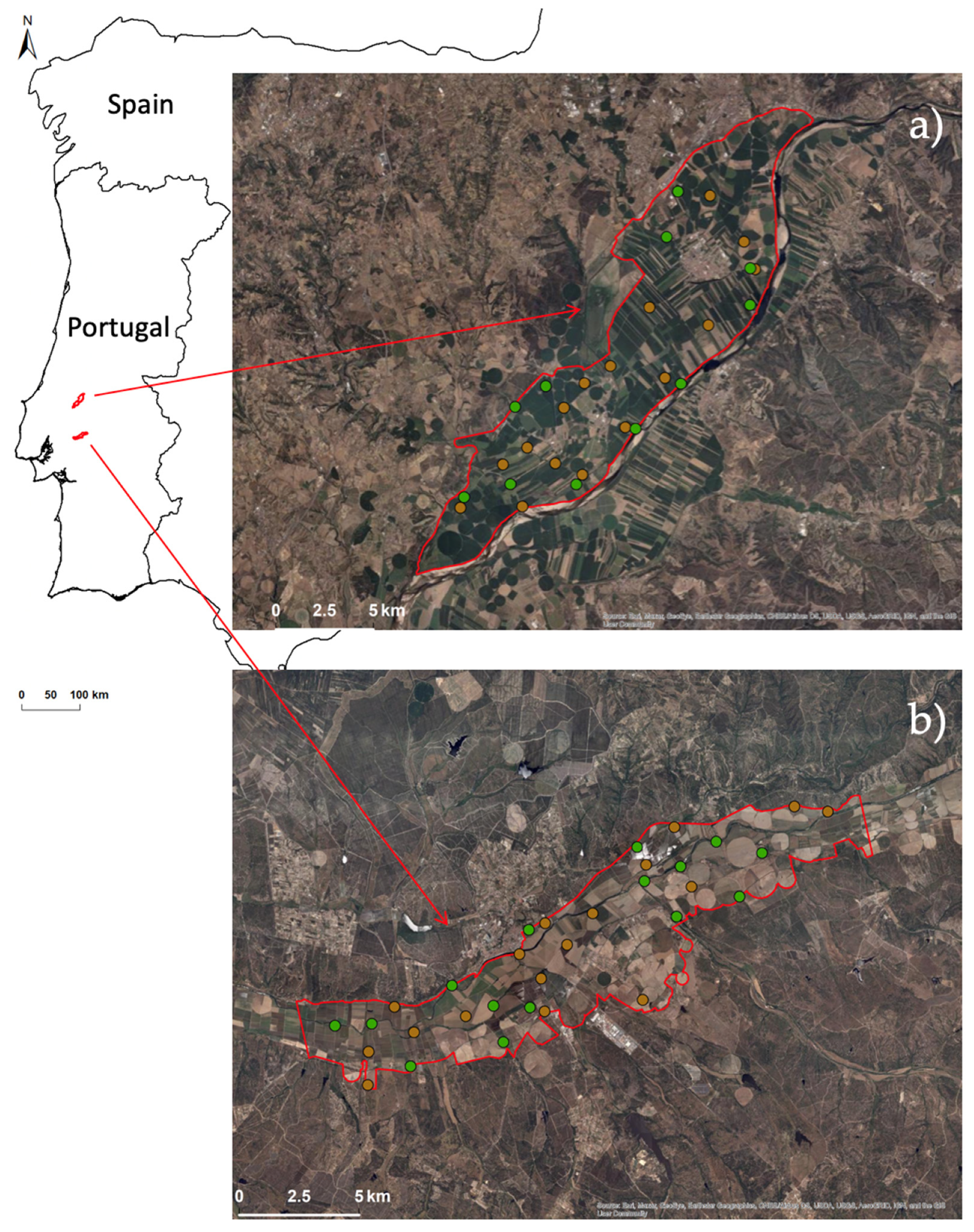
2.1. Study Area

The study was carried out in 2019 in two irrigated agricultural areas of central Portugal, located in Sorraia and Tagus valleys (central point coordinates: Lat. 38.9581 Long. −8.52837, Lat. 39.4027 Long. −8.48908, respectively; Figure 1). The two study areas are spread over the floodplain zone of rivers Sorraia and Tagus, dominated by intensive agricultural systems composed of annual crops, with a predominance of rice paddies (Oryza sativa L.) in the alluvial plains of the Sorraia river, and maize fields (Zea mays L.) in the Tagus River valley. The Sorraia valley is enclosed by an agroforestry system characterized by open canopy woodlands, mainly dominated by cork oak (Quercus suber L.) and holm oak (Q. ilex spp. rotundifolia Lam.), with an undercover of seminatural grasslands, traditionally exploited by multiple land uses, including pastures and cereal crops [45]. The Tagus valley is surrounded by a forest production system, characterized by mixed forestland composed mainly of blue gum (Eucalyptus globulus Labill.) plantations, occasional stands of maritime pine (Pinus pinaster Aiton), and near-natural cork oak forest remnants, with shrubby vegetation strata dominated by Hakea sericea Schrad. & J.C.Wendl. and Cystus ladanifer L. Both areas exhibit scattered human settlements.
The climate in the region is characterized by mild winters and hot, dry summers with frequently irregular interannual fluctuations of precipitation. Flood peaks usually occur in early winter, followed by a slowly declining flow and a consequent drying during late spring and summer. The annual average precipitation and temperature range between 600–800 mm and 15–17.5 °C, respectively [46].

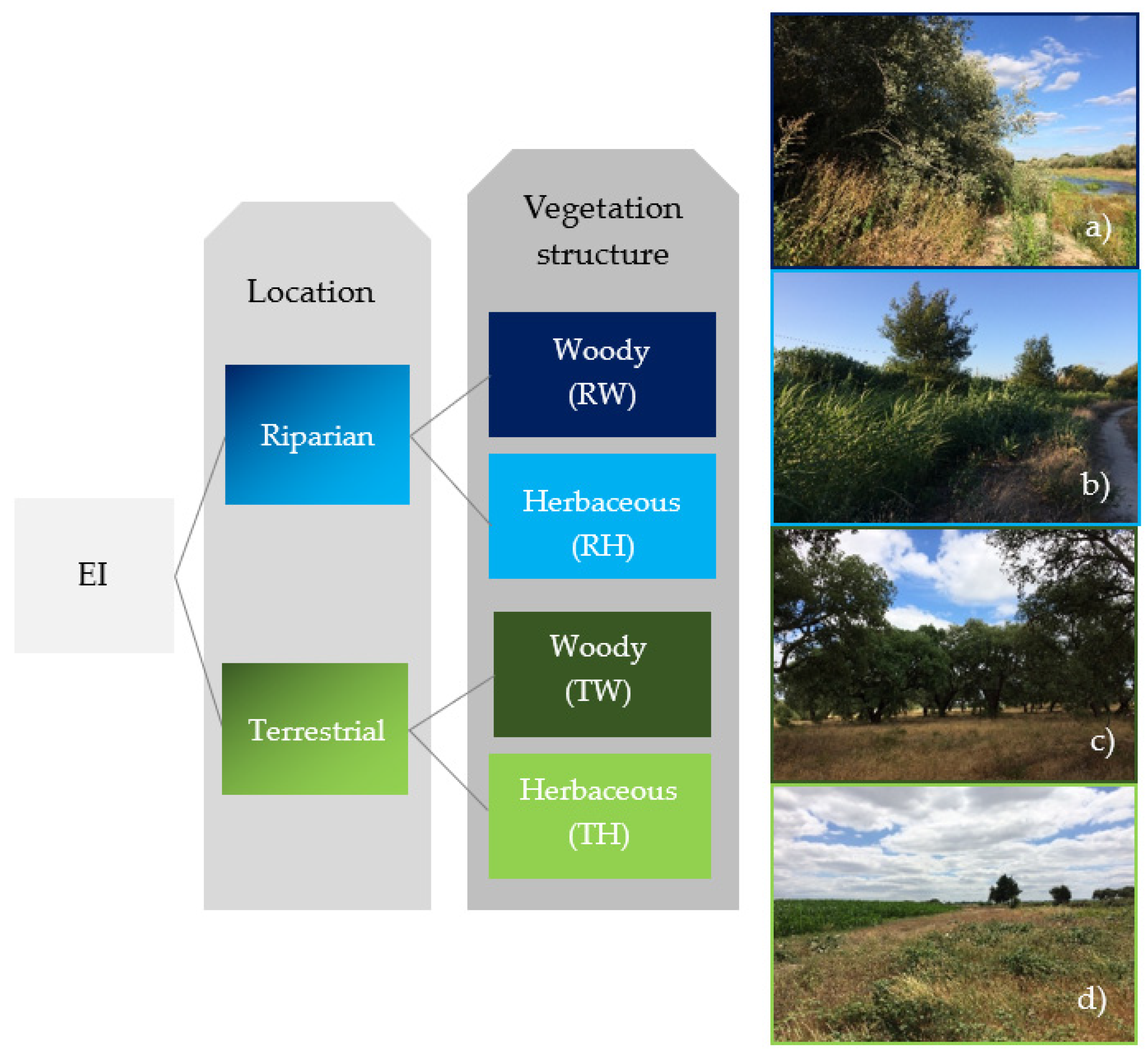
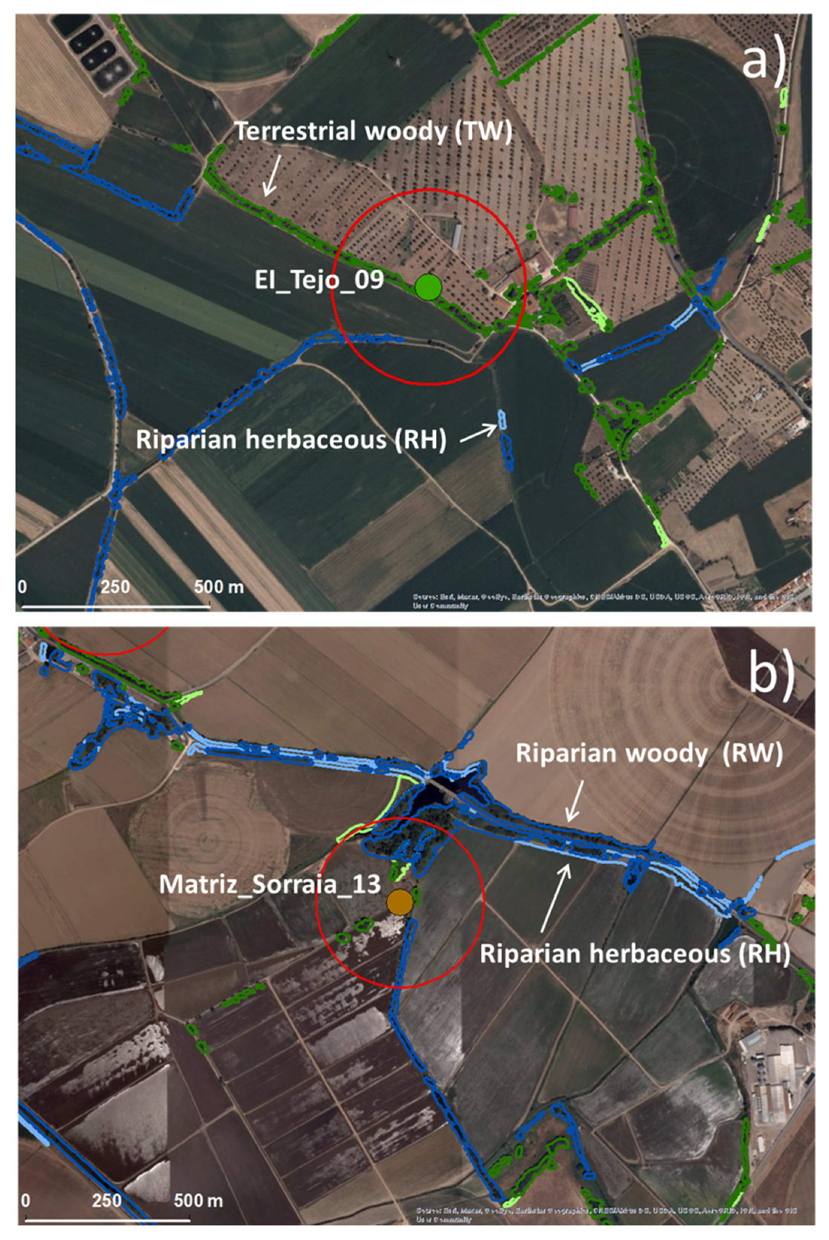
2.2. Ecological Infrastructures Classification System and Mapping

We only considered permanent EIs, consisting of homogenous vegetation patches differing from their surroundings in terms of origin and dynamics and established in the field for more than one year. We first classified EIs according to their location, based on a gradient of water proximity, i.e., riparian vs. terrestrial. We then divided the former classes according to their vegetation structure, based on the dominant strata, i.e., woody vs. herbaceous. Four classes were thus defined, hereafter designated as riparian woody (RW), riparian herbaceous (RH), terrestrial woody (TW), and terrestrial herbaceous (TH) (Figure 2). The RW class includes all the trees and tall shrub vegetation patches surrounding river systems, from the edge of the stream bank to the external limit of the canopy, where an abrupt change in vegetation composition, height, type, and amount occurs [47,48]. The RH class includes open areas at the riparian zone, mostly dominated by herbaceous vegetation and some low shrubs. The TW class includes all patches of tree-dominant vegetation found in terrestrial ecosystems, while the TH class includes open areas mostly dominated by herbaceous vegetation. EIs area was on average 8.1 ± 2.5 ha ranging between 0.03 and 31.91 ha.
An image-based approach supported by a Geographic Information System was used to map, store, and organize all the landscape information. EIs were obtained by manually digitalizing the vegetation patches through visual classification of the World Imagery layer (ArcGIS Online data, Copyright © Esri), obtained in 2018, with a spatial resolution of 0.6 m. The vegetation polygons were digitized at a 1:1000 scale and selected the Minimum Mapping Unit of 200 m2, with a minimum width of 5 m and a minimum gap between vegetation patches of 10 m.

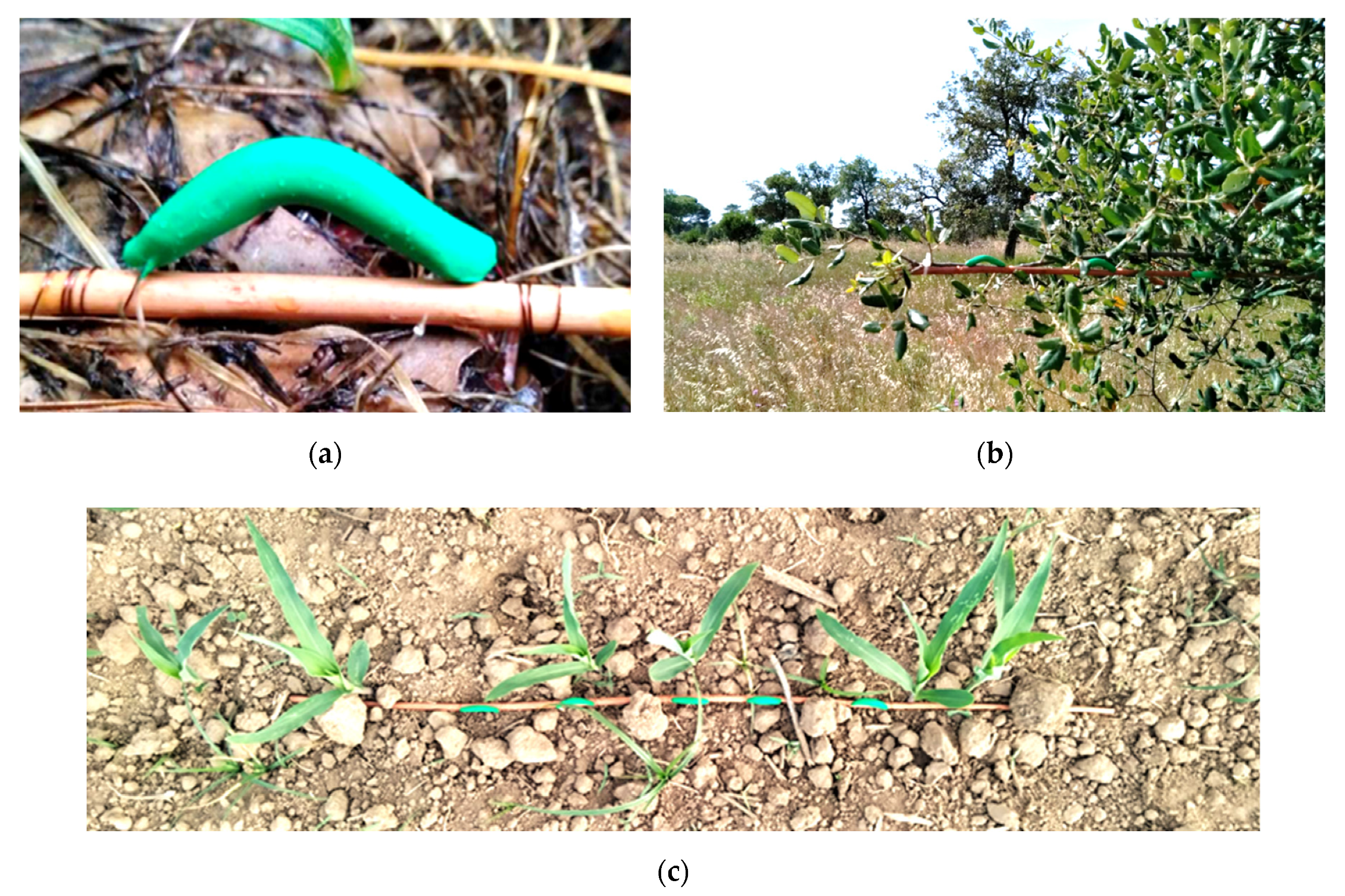
2.3. Dummy Caterpillars

Dummy caterpillars were made of green clay plasticine (Staedtler, Noris Club 8421), mimicking the size and shape of real lepidopteran larvae (caterpillars), with an inchworm curved shape, about 3 cm long [30] (Figure 3a). To avoid contamination with human scent, all dummy caterpillars were prepared and handled with gloves.

2.4. Field Experimental Design

Dummy caterpillars were installed in both EIs (Number of sites, N = 26) and agricultural matrix (N = 34) in May 2019, covering different landscape elements (Figure 1), and distributed between the two study areas: Sorraia (N = 32) and Tagus (N = 28). Sampling sites were separated by at least 500 m to avoid spatial autocorrelation. We installed 10 dummy caterpillars per site, corresponding to 600 dummies in total. This number is in the range of sentinel prey per experiment reported in a review by Lövei and Ferrante [49] (median = 658.5; range = 32–14,400, n = 46).
The central point of each sampling site was geo-referenced using a GPS with an estimated accuracy of less than 3 m. Two wicker sticks with five dummy caterpillars each spaced ca. 10 cm distance were placed either on (1) the tree canopy attached to branches at 1.5–1.8 m height (Figure 3b) or (2) on the ground level, fixed with tent pegs (Figure 3c). To keep the caterpillars in place, a thin thread was passed through them, and their ends wrapped around the wicker [30]. Dummy caterpillars were recovered after 30-day exposure in the field and individualized per site into small cardboard boxes with a paper fan, including a label registering the site, EI typology, or agricultural matrix for posterior study in the laboratory.

2.5. Assessment of Bird Species Assemblages

A survey was carried out to determine the species composition of bird communities as a case study among the different predator guilds. For that, abundance measurements were carried out for all recorded bird species (point counts) in 41 sites located within the Tagus valley. The sampling sites were distributed between the agricultural matrix (N = 20) and the woody EIs (N = 21). All species sightings or vocalizations within less than 30 m from the observation point were recorded. The avifauna was identified and counted for 10 min at each point. Study sites were visited in the morning, from 6:00 a.m. to 11:00 a.m., and in the afternoon, from 4:00 p.m. to 7:00 p.m., during April and May 2019, coinciding with the reproductive period. The information about insect consumption by bird species was retrieved from Billerman et al. [50].

2.6. Identification and Quantification of Predation Marks on Dummy Caterpillars

The dummy caterpillars were observed in the laboratory, and predation marks were analyzed under magnification (Optika SZM.LED1 stereomicroscope, 7×–45×). The type of predation mark (i.e., insect, bird, mammal) was identified according to the signs left by the predator’s mandibles, teeth, beak, or ovipositor, based on Howe et al. [35] and Low et al. [30] descriptions and model images. Insect marks may include scratching, stabs, holes, slits, and gouges; bird attacks result in pecks and gouges, u- or v-shaped occurring on both sides of the model with more vigorous attacks resulting in chunks being taken out, while mammal attacks are evident from teeth impressions including small paired incisor marks occurring on both sides of the models corresponding to upper and lower jaw [30]. The number of marks per caterpillar was recorded.
Cross validation of the identification process was carried out by two observers based on a sample of about 12% of the total number of dummies. Each observer independently recorded their observations and posteriorly compared the results together. After this calibration, one observer studied all dummies and registered their predation marks. Then, the second observer made a double check, passing over all dummies.

2.7. Landscape Variables

Two circular buffers with 200 m and 500 m radius were considered, surrounding the center of each sampling site, using the GPS coordinates (Figure 4). Buffer featuring is an important methodological approach for the identification of landscape–species relationships [51,52]. In addition to location and vegetation structure, EIs were characterized using landscape metrics, such as area and percentage area, within each buffer size. We additionally calculated the mean and minimum distance for sampling sites located in the agricultural matrix to the nearest EI.

2.8. Statistical Analyses

A Generalized linear mixed model (GLMM) was used to determine whether the predation rate was higher on EIs compared with the agricultural matrix and whether predation differed according to EIs typologies, namely their location (riparian vs. terrestrial) and structure (woody vs. herbaceous). Models were fitted to the target overall predation rate, as well as the predation rate by different groups of predators (birds, mammals, and insects). The study area was included as a random effect to account for sources of variability between the two irrigated valleys. The target variables were expressed as the percentage of dummies predated (predation rate). Binomial distribution and log link were used. Pairwise contrasts were performed based on the least significant difference adjusted (α = 0.05). Pearson correlation was estimated to the analyzed relationship between landscape variables and predation rate per site for each group of predators. All tests were carried out using IBM SPSS [53]. Results are presented as means ± standard error unless otherwise mentioned.

3. Results

3.1. Bird Species Observed

Bird fauna at the studied area consisted of 28 species and 26 genera from 15 families in the Passeriformes order (Table 1). The number of observed species and individuals in EIs was 1.5 and 2.0 times higher than that in the agricultural matrix, respectively. About 82% of the identified bird species are known to prey on lepidopteran species (Table 1). Among these species, 14 occurred in both studied habitat typologies, 13 foraged in open fields, and 16 were tree-dependent for foraging or nesting (Table 1).

3.2. Overall Predation Pressure

We recovered 576 from the 600 dummy caterpillars installed in the experiment. Twenty-four dummies (4%) were damaged by machinery and other unidentified causes and thus not considered for determining the number of predation marks. One sampling site from the agricultural matrix of the Tagus basin was completely removed. The total number of predation marks was 643. Overall predator attack rate was 33.0 ± 3.8% per 30 days, integrating the predation activity of birds (11.2 ± 2.5%), mammals (14.5 ± 2.7%), and insects (11.7 ± 2.4%). The estimated attack rate per day of the exposed dummy caterpillars was 1.1%, 0.4%, 0.5%, and 0.4% for total predators, birds, mammals, and insects, respectively.

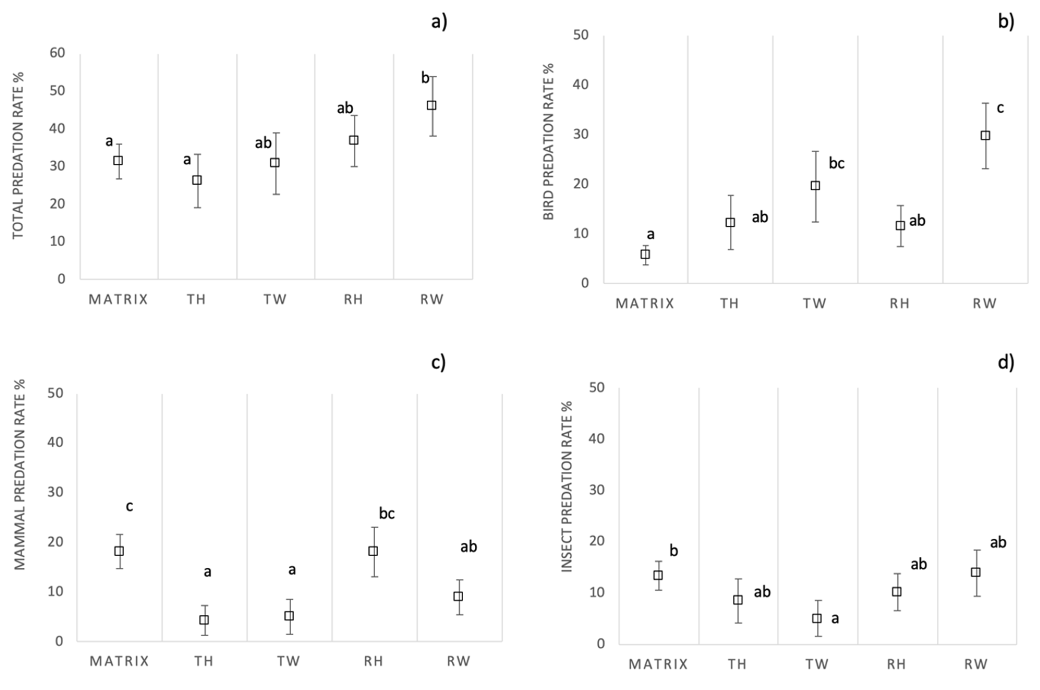
3.3. Predation Rate in Ecological Infrastructures Versus Agricultural Matrix

Overall predation rate did not differ between matrix (37.4 ± 5.4%) and EI sites (31.1 ± 4.9%) (t574 = 1.401, p = 0.162). However, different patterns were found for the different predator groups, when comparing EIs with the agriculture matrix. Predation rate registered for birds was about three times higher in EIs (18.7% ± 3.5) than in the agricultural matrix (5.9% ± 1.7) (t574 = 4.670, p < 0.001). Oppositely, the attack rate by mammals was lower on EIs (10.7% ± 2.3) in comparison with the agricultural matrix (18.0% ± 2.8) (t574 = −2.444, p = 0.015). No significant differences were observed in the case of insects (t574 = −1.156, p = 0.248).

3.4. Predation Rate in Different Ecological Infrastructures’ Typologies

When analyzing sites by typologies, the predation rate showed an increasing trend from the lowest levels in the TH sites towards the highest in RW ones (Figure 5a). Still, pairwise differences were significant only between RW and agricultural matrix sites (t571 = 2.284, p = 0.023), as well as between RW and TH sites (t571 = 2.253, p = 0.025).
Again, different trends were observed in each predator guild. Bird predation rates differed among site typologies (F4,571 = 8.204, p < 0.001), being higher in woody EIs (TW and RW) than in other site typologies (Figure 5b). Comparisons among RW and all other site typologies were significant, except for TW (Figure 5b). On the other hand, the predation rate in TW differed from that in the agricultural matrix (t571 = 2.166, p = 0.031), but not from those in the other EIs typologies.
Overall predation rate by mammals also differed with site typologies (F4,571 = 2.614, p = 0.034). Mammal predation rate was highest in the agricultural matrix and RH sites. The lowest values were observed in the two terrestrial EIs types (Figure 5c). Insect predators showed less variation among site typologies with no overall significant fixed effect (F4,571 = 0.812, p = 0.518). Nonetheless, the pairwise comparison showed that the predation rate by insects in the agricultural matrix was significantly higher than in TW sites (t571 = 2.039, p = 0.042) (Figure 5d).

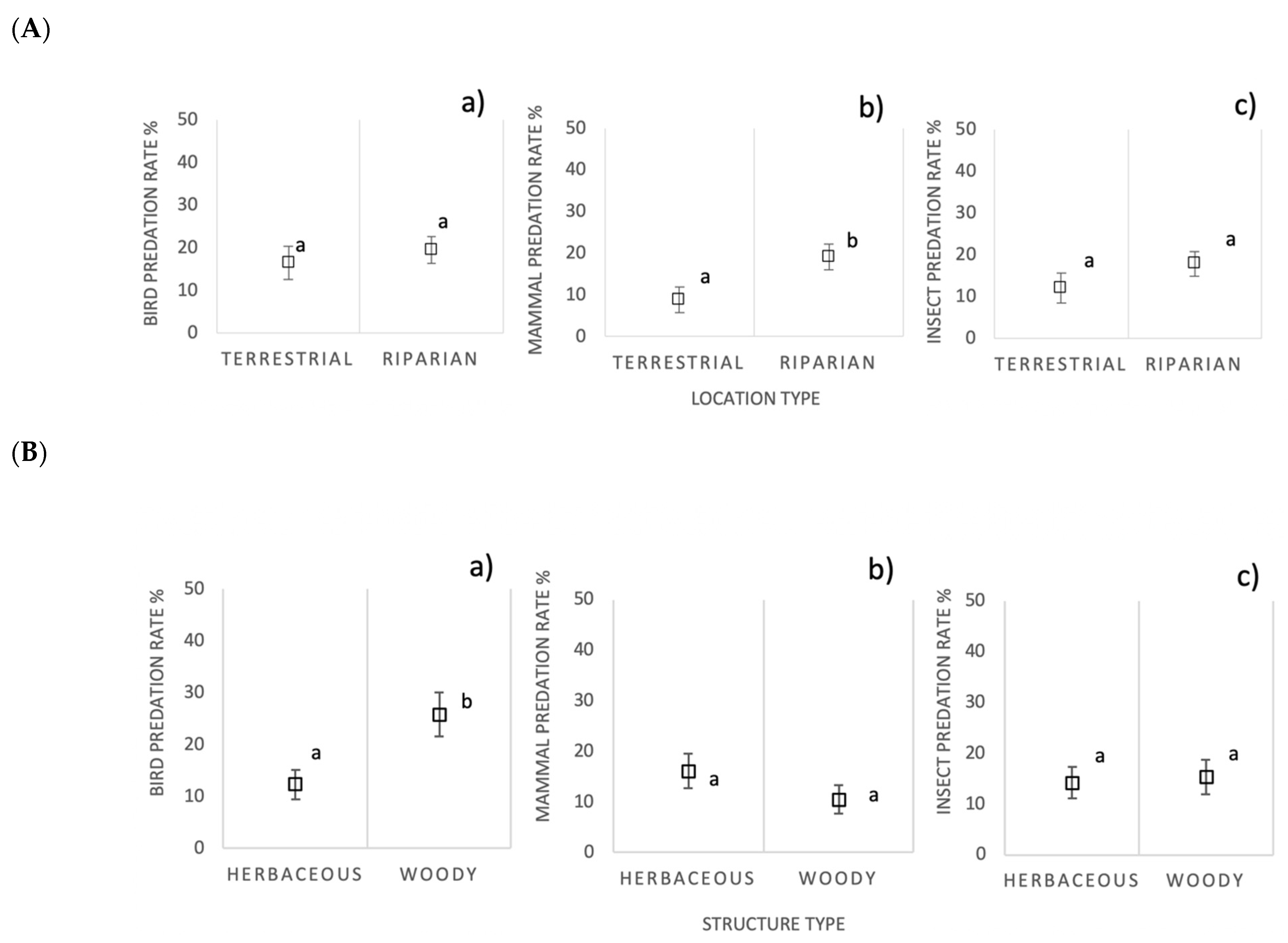
3.5. Predation by Ecological Infrastructure Location and Vegetation Structure

The different groups of predators had contrasting results regarding EIs location (riparian vs. terrestrial) and structure (woody vs. herbaceous). Predation rates tended to be higher on riparian EIs in comparison with terrestrial ones for all predator guilds (Figure 6). Still, the differences were significant for mammals (F1,252 = 4.261, p = 0.040), but not for birds (F1,252 = 0.037, p = 0.544) or insects (F1,252 = 1.358, p = 0.245).
Bird predation rate was mostly affected by the EI structure, being higher in woody than in herbaceous EIs (F1,252 = 7.372, p = 0.007) (Figure 6). However, EI structure did not affect predation rate by mammals (F1,252 = 2.095, p = 0.149) or insects (F1,252 = 0.083, p = 0.773) (Figure 6).

3.6. Landscape Metrics

Considering all sites (N = 59), the mean percentage of area covered by EIs in the 200 m buffer was 9.5 ± 1.3%, ranging between 0 and 52%. About 95% of the sites had less than 30% of the area covered by EIs. In the 500 m buffer, the mean percentage of area covered by EIs was 5.5 ± 0.6%, ranging between 0 and 19%.
As for the agricultural matrix sites (N = 33), the mean percentage of area occupied by EIs was 5.9 ± 1.2% (ranging between 0 and 22%), for the 200 m buffer, and 4.5 ± 0.8% (ranging between 0 and 19%), for the 500 m buffer.
The predation rate by birds was positively correlated with the area occupied by EIs in the surrounding landscape. This was observed for all types of EIs at 500 m, as well as when considering only the woody or the riparian individually, at both 200 m and 500 m buffers (Table 2). In addition, significant negative correlations were found between the distance to the nearest riparian and nearest woody EIs and bird predation rate. Mammal predation rate displayed a positive correlation with distance to the nearest woody EI. Insect predation rate did not show any significant correlation with the landscape variables. Distance to river was negatively correlated with bird predation rate (r = −0.326, p = 0.012), but not with mammal (r = −0.049, p = 0.714) or insect predation rates (r = −0.145, p = 0.275).
Considering only the agricultural matrix sampling sites, we also found a positive correlation between the predation rate by birds and the area covered by EIs in the landscape. Correlations were significant for the total area covered by EIs at 200 m and 500 m, as well as when considering only the riparian EI at 500 m and woody EI at both 200 m and 500 m buffers (Table 2). Nevertheless, the level of correlation was higher in the 500 m buffer than in the 200 m buffer. For mammal and insect predation rates, no significant correlation was found with the area covered by EIs in the landscape.
Regarding EI sampling sites (N = 26), we further found a positive correlation between the specific area of the EI where the dummies were located and the bird predation rate (r= 0.572, p = 0.002). This was not observed for mammal (r = −0.023, p = 0.258) or insect predation rates (r = 0.057, p = 0.782).

4. Discussion

4.1. Overall Predation Pressure

Artificial caterpillars have been used as prey sentinels to estimate predation rates of both vertebrate and invertebrate predators in multiple studies [32,54,55]. Due to its simplicity in relation to real prey, the method has been proposed for assessing the invertebrate predation service [49,56].
Lövei and Ferrante [49] reviewed the use of sentinel prey to estimate invertebrate predation. Based on the analysis of 42 articles using artificial caterpillars, they determined a median attack rate of 8.8% per day for predators in general, 3.9% per day for vertebrate predators, and 3.3% per day for invertebrate predators. In our study, the estimated attack rates of the exposed dummy caterpillars were lower than the median values reported by Lövei and Ferrante [49], although within the range of reported values. These results suggest that the predation pressure in the study systems is relatively low. By using caterpillar dummies, we also underestimate the activity of insect predators that prey on other developmental insect stages, such as eggs and pupae. We also admit that the predation rate per day might be underestimated in our study because of the relatively long exposure period of the experiment (30 days). Another explanation could be that only one size of artificial caterpillar was used. Whereas birds are not affected by prey body size and are more likely to attack larger caterpillars [57], arthropod predators may be in a biased position since they tend to be more successful when attacking smaller caterpillars [58]. Nevertheless, birds dominate in temperate ecosystems, while insects, namely ants and wasps, are the main predators in tropical forests [58,59,60].

4.2. Effects of Ecological Infrastructures and Landscape Metrics on Predation Rate

EIs have been reported to support functional biodiversity and related ES in agricultural systems [13,14,24,61]. Concerning ES related to regulatory predation, most studies analyze predators’ abundance and diversity supported by EIs in the vicinity of agricultural fields [13,27]. Differences in the composition of predator communities in function to different types of EIs have also been observed [13]. However, the influence of EIs on insect predation is still poorly studied. In addition, the effects of vegetation structure, EIs proportion in the landscape, and other elements, such as the proximity to riverine habitats, have not been comprehensively studied. The effects of EI structure and location may also differ between predatory groups. In our study, we used predatory attacks of three different predator guilds (birds, mammals, and insects) to artificial sentinel prey as a proxy of the predation service in irrigated agricultural areas in a Mediterranean region to understand some of those effects.
We hypothesized that EIs would provide a variety of habitats, shelters, and prey because of the diversity of host plants and resources, depending on their typologies. Therefore, we were expecting that: (i) EIs would promote the abundance of predators, which would be reflected in a higher predation rate in comparison with the agricultural matrix; (ii) the predicted positive effect of EIs on predation would be influenced by the structure, location, and spatial configuration of EIs; and (iii) the predation rate would be higher in the agricultural fields in the vicinity of EIs and with a higher proportion of EIs in the surrounding landscape. Overall, our results support these predictions, but only for birds. Specific and contrasting effects were observed for other predatory guilds. Previous studies have also found contrasting effects of the natural and seminatural habitat configuration and typology for different taxa, and therefore there is currently no consensus about the importance of EIs spatial variables to the distinct biological groups [62,63]. In our work, one of the most relevant results was that EI vegetation structure (woody vs. herbaceous) and location (riparian vs. terrestrial) impacted the three groups of predators (birds, mammals, and insects), as well as the overall predation rate.
Insect predation by birds contributed to the overall differences observed between EIs and the agricultural matrix. The higher number of insectivorous bird species associated with EIs (22 species), compared with the agricultural matrix (15 species), is in line with the observed differences in predation rate. The predation rates originated by birds were mostly linked with woody habitats, both riparian and terrestrial. In fact, about 62% of the bird species observed in the study area associated with EIs are lepidopteran predators and tree-dependent species for foraging and nesting. Further, the highest predation by birds was observed in trees in the vicinity to the water, i.e., riparian woody, also corresponding to more complex vegetation structural composition. Riparian habitats also provide emergent aquatic insect populations that may constitute an alternative food source for insectivorous birds [64]. It has been shown that riverine structures support high bird diversity, species that are sensitive to riparian vegetation structure and composition [65]. The importance of riparian habitats in supporting regulatory ES, such as pollination and pest control, has been highlighted [16,66,67].
Mammal attack rates were highest in riparian habitats, in particular herbaceous. Other studies showed that riparian habitats may work as shelter areas and result in higher diversity and abundance of small mammals [68,69]. This effect increases in tandem with the greater complexity of vegetation structure [68]. Also striking was to observe that predation by mammals was higher in the agricultural matrix than in most of the EIs, except the riparian herbaceous. We suspect this might be associated with the presence of small omnivorous rodents in maize crops, often attracted by seed consumption. For instance, voles abundance may be influenced by crop characteristics such as density and height [70]. The response differences between groups of predators may be related to habitat usage and functional connectivity among habitats. On the other hand, the overall low predation rates are possibly related to the intensive agricultural system studied and the relatively low percentage of the studied area covered by EIs, which was estimated to be on average about 5.5%, including forest areas, and about 4.5%, in the agricultural matrix (for the larger buffer considered, i.e., 500 m). According to Boller et al. [12], the optimal total surface covered by natural habitats to support adequate functional biodiversity in agricultural systems is estimated to be around 15%. A minimum of 5% of the farm surface covered by EIs, excluding forests, is required by the International Organization for Biological and Integrated Control (IOBC) as a guideline for integrated production [71]. With a relatively low level of EIs in the landscape, it is expected to have higher habitat fragmentation, with a higher mean distance between EI patches. We will expect that the mobility of predator species with lower dispersal capacity will be most affected because of lower connectivity. This is the case of predatory insects and small mammals in comparison to insectivorous birds. Many of these beneficial species have a limited dispersion range, up to 100–200 [12,72,73,74,75], whereas bird species tend to show higher mobility [76]. Our findings, which showed a positive correlation between predation rate and the area covered by EIs in the surrounding landscape, for both 200 m and 500 m buffers, and a negative correlation with the distance to the nearest riparian and woody EIs, support those predictions, only in the case of birds. This is in line with Boesing et al. [77] findings, where land-use heterogeneity, enhanced native habitat amount, and proximity to native habitat patches were all positively linked to pest suppression, based on a literature review on the effects of landscape structure on bird-mediated pest control.

4.3. Drawbacks and Strengths of the Method

Dummy caterpillars allow for a standardized and rapid assessment of relative predation rates. They are easy to install and to assess, being also appropriate for citizen science programs [78]. Quantification of invertebrate predation is not easy, as evidence is difficult to obtain [35,79]. In contrast, dummies allow collecting predator’s marks and can be implemented on a large scale and diversity of habitats. Dummy caterpillars have been increasingly used with the main purpose of measuring variation in predation pressure. The method has proven to give comprehensible results in different contexts, such as when comparing predator variations between canopy and understory habitats [36], forest gaps, and forest understory [80], variation across different types of forests [32], different agricultural land-uses [37], along urbanization gradients [29], elevation [31] or latitudinal variation [78,79,81]. Still, the interpretation of the results must be considered carefully. Differences in predation activity may be expected when changing the exposition of the caterpillars, such as naturally exposed vs. semiconcealed mimicking leaf-rolling caterpillars [82]. In addition, the presence of particular elements of the microhabitat or avoidance of local predators might influence the results. For example, Dáttilo et al. [83] showed that predators were visually repelled by ants, reducing predation marks on dummy caterpillars near objects resembling ant shapes.
Dummies are inactive and inodorous, which may make them less attractive to predators and thus might not reflect natural predation rates [34,35]. On the other hand, dummies do not run away or hide from threats, which may be considered to create a conservative balance [35]. Still, we need to consider that dummies attract predators merely by visual cues. Different groups of predators are more oriented by visual cues than others and may respond in different ways to the color, size, and shape of the prey. Thus, despite being a similar technique, the results among groups have to be compared carefully. In particular, birds are probably mostly attracted by prey visual cues (color and shape) and less by odors, as birds mainly use vision to perceive information from their environment [84]. On the contrary, for many predator insect species, in particular specialist ones, vibrational and chemical cues play a major role while searching for prey as well as for prey recognition and acceptance. Chemical cues may include semiochemicals emitted directly by the prey (e.g., [85,86]) or associated with the prey, such as feces (e.g., [87]) or plant volatiles [88]. Small mammals are also acoustically oriented to locate and select their prey [89]. The differential response of birds observed in our study, in comparison to insects and mammals, could be in part due to different prey detection and recognition mechanisms used by these three predator groups. Bird marks are also probably more reliable than insect marks, as they are easier to distinguish even by nonexpert observers [90].
Finally, we may assume that dummy visibility may depend on the habitat itself. For example, a dummy exposed in an open field may be more visible than in dense vegetation. It should be taken into consideration that in our study, the arrangement provided for woody habitats and nonwoody was not the same. In woody habitats, dummy caterpillars were placed on the tree canopy attached to branches ca. 1.50 m height, whereas in herbaceous habitats or the agricultural matrix, dummies were placed on the ground. Nevertheless, no differences in the predation rate were observed between herbaceous and woody EIs, both terrestrial and riparian, suggesting that dummies’ position did not affect the results.

5. Conclusions

Overall, we observed a consistent trend of increasing predation from agricultural matrix to complex and biodiverse systems, such as the riparian woody EIs. However, we observed differences between groups of predators. The birds were the most responsive to the proximity and area covered by woody EIs in the landscape. The presence and proximity to riparian EIs were also important factors for predation by birds. Insects were the least responsive predator group to habitat complexity. The observed differential response of the studied predators is possibly related to the low proportion of EIs in the landscape, with low connectivity levels for the less mobile predator groups, such as insects. Future studies should consider different landscapes with different levels of EIs to test this hypothesis. Finally, our results should be interpreted with some caution, considering the limitations of the method and that they are based on one-year sampling.

Author Contributions

Conceptualization, J.C.F., M.B., G.D., A.F., V.Z., M.R.F. and M.T.F.; field sampling, S.C., A.F., G.D., T.M., J.L.S. and V.Z.; laboratory identification, S.C., A.G. and M.B.; formal analysis, M.B. and J.C.F.; writing—original draft preparation, S.C., J.C.F. and M.B.; writing—review and editing, J.C.F., M.B., M.R.F., G.D., A.G., S.C., A.F., V.Z. and M.T.F.; project administration, G.D., M.R.F. and M.T.F. All authors have read and agreed to the published version of the manuscript.

Funding

This research was funded by CERES Interreg, grant number IV-B SUDOE-SOE2/P5/F0551.

Institutional Review Board Statement

Not applicable.

Informed Consent Statement

Not applicable.

Data Availability Statement

Not applicable.

Acknowledgments

We are grateful to the stakeholders and the farmers’ associations (Agrotejo and Associação de Regantes e Beneficiários do Vale do Sorraia—ARBVS) for all the support during fieldwork. We would like to express a special thanks to Susana Rocha for assistance in the field and Sofia Branco, Ana Farinha, and Miguel Pereira for the help in molding the dummies. This research also received backing from Optimus Prime (FCT-PTDC/ASP-AGR/29771/2017), Forest Research Centre (CEF), a research unit funded by Fundação para a Ciência e a Tecnologia (FCT), Portugal, grant number UIDB/00239/2020 and Laboratory for Sustainable Land Use and Ecosystem Services—TERRA (LA/P/0092/2020). GD was supported by national funds via FCT (PTDC/ASP-AGR/29771/2017 and UIDP/00239/2020). AF and VZ were supported by national funds via FCT (PD/BD/142884/2018 and PD/BD/142882/2018, respectively). SC was supported by EU funds via a research grant under the CERES project. AG was supported by European Union’s Horizon 2020 Program for Research and Innovation under grant agreement no. 771271 ‘HOMED’.

Conflicts of Interest

The authors declare no conflict of interest.

References

  1. Foley, J.A.; DeFries, R.; Asner, G.P.; Barford, C.; Bonan, G.; Carpenter, S.R.; Chapin, F.S.; Coe, M.T.; Daily, G.C.; Gibbs, H.K.; et al. Global consequences of land use. Science 2005, 309, 570–574. [Google Scholar] [CrossRef] [PubMed] [Green Version]
  2. Garbach, K.; Milder, J.C.; Montenegro, M.; Karp, D.S.; DeClerck, F.A.J. Biodiversity and Ecosystem Services in Agroecosystems. Encycl. Agric. Food System 2014, 2, 21–40. [Google Scholar] [CrossRef]
  3. Cole, L.J.; Brocklehurst, S.; Robertson, D.; Harrison, W.; McCracken, D.I. Exploring the interactions between resource availability and the utilisation of semi-natural habitats by insect pollinators in an intensive agricultural landscape. Agric. Ecosyst. Environ. 2017, 246, 157–167. [Google Scholar] [CrossRef]
  4. Benton, T.G.; Vickery, J.A.; Wilson, J.D. Farmland biodiversity: Is habitat heterogeneity the key? Trends Ecol. Evol. 2003, 18, 182–188. [Google Scholar] [CrossRef]
  5. Holland, J.M.; Bianchi, F.J.; Entling, M.H.; Moonen, A.-C.; Smith, B.M.; Jeanneret, P. Structure, function and management of semi-natural habitats for conservation biological control: A review of European studies. Pest Manag. Sci. 2017, 72, 1638–1651. [Google Scholar] [CrossRef]
  6. Hannon, L.E.; Sisk, T.D. Hedgerows in an agri-natural landscape: Potential habitat value for native bees. Biol. Conserv. 2009, 142, 2140–2154. [Google Scholar] [CrossRef]
  7. Cole, L.J.; Brocklehurst, S.; Robertson, D.; Harrison, W.; McCracken, D.I. Riparian buffer strips: Their role in the conservation of insect pollinators in intensive grassland systems. Agric. Ecosyst. Environ. 2015, 211, 207–220. [Google Scholar] [CrossRef]
  8. Martin, E.A.; Dainese, M.; Clough, Y.; Báldi, A.; Bommarco, R.; Gagic, V.; Garratt, M.P.; Holzschuh, A.; Kleijn, D.; Kovács-Hostyánszki, A.; et al. The interplay of landscape composition and configuration: New pathways to manage functional biodiversity and agroecosystem services across Europe. Ecol. Lett. 2019, 22, 1083–1094. [Google Scholar] [CrossRef] [Green Version]
  9. Sanaullah, M.; Usman, M.; Wakeel, A.; Cheema, S.A.; Ashraf, I.; Farooq, M. Terrestrial ecosystem functioning affected by agricultural management systems: A review. Soil Tillage Res. 2020, 196, 104464. [Google Scholar] [CrossRef]
  10. Pecheur, E.; Piqueray, J.; Monty, A.; Dufrêne, M.; Mahy, G. The influence of ecological infrastructures adjacent to crops on their carabid assemblages in intensive agroecosystems. PeerJ 2020, 8, e8094. [Google Scholar] [CrossRef]
  11. Silva, J.M.C.; Wheeler, E. Ecosystems as infrastructure. Perspect. Ecol. Conserv. 2017, 15, 32–35. [Google Scholar] [CrossRef]
  12. Boller, E.F.; Hani, F.; Poehling, H.M. Ecological infrastructures. In Ideabook on Functional Biodiversity at the Farm Level; IOBC/wprs: Lindau, Switzerland, 2004. [Google Scholar]
  13. Rosas-Ramos, N.; Baños-Picón, L.; Tobajas, E.; de Paz, V.; Tormos, J.; Asís, J.D. Value of ecological infrastructure diversity in the maintenance of spider assemblages: A case study of Mediterranean vineyard agroecosystems. Agric. Ecosyst. Environ. 2018, 265, 244–253. [Google Scholar] [CrossRef]
  14. Rosas-Ramos, N.; Baños-Picón, L.; Trivellone, V.; Moretti, M.; Tormos, J.; Asís, J.D. Ecological infrastructures across Mediterranean agroecosystems: Towards an effective tool for evaluating their ecological quality. Agric. Syst. 2019, 173, 355–363. [Google Scholar] [CrossRef]
  15. Naiman, R.J.; Decamps, H.; Pollock, M. The role of riparian corridors in maintaining regional biodiversity. Ecol. Appl. 1993, 3, 209–212. [Google Scholar] [CrossRef] [PubMed]
  16. Riis, T.; Kelly-Quinn, M.; Aguiar, F.C.; Manolaki, P.; Bruno, D.; Bejarano, M.D.; Clerici, N.; Fernandes, M.R.; Franco, J.C.; Pettit, N.; et al. Global overview of ecosystem services provided by riparian vegetation. BioScience 2020, 70, 501–514. [Google Scholar] [CrossRef]
  17. European Commission. Communication to the European Parliament, the Council, the European Economic and Social Committee and the Committee of the Regions: Green Infrastructure (GI)—Enhancing Europe’s Natural Capital; European Commission: Brussels, Belgium, 2013. [Google Scholar]
  18. European Commission. The EU Guidance Document on Integrating Ecosystems and Their Services in Decision-Making; European Commission: Brussels, Belgium, 2013. [Google Scholar]
  19. European Commission. Report from the Commission to the European Parliament and the Council on the Implementation of the Ecological Focus Area Obligation under the Direct Payment Scheme; European Commission: Brussels, Belgium, 2017. [Google Scholar]
  20. European Commission. EU Guidance Document on a Strategic Framework for Further Supporting the Deployment of EU-Level Green and Blue Infrastructure SWD, 193 Final; European Commission: Brussels, Belgium, 2019. [Google Scholar]
  21. Cole, L.J.; Kleijn, D.; Dicks, L.V.; Stout, J.C.; Potts, S.G.; Albrecht, M.; Balzan, M.V.; Bartomeus, I.; Bebeli, P.J.; Bevk, D.; et al. A critical analysis of the potential for EU Common Agricultural Policy measures to support wild pollinators on farmland. J. Appl. Ecol. 2020, 57, 681–694. [Google Scholar] [CrossRef] [PubMed]
  22. Heyl, K.; Döring, T.; Garske, B.; Stubenrauch, J.; Ekardt, F. The Common Agricultural Policy beyond 2020: A critical review in light of global environmental goals. Rev. Eur. Comp. Int. Environ. Law 2021, 30, 95–106. [Google Scholar] [CrossRef]
  23. Rotchés-Ribalta, R.; Ruas, S.; Ahmed, K.D.; Gormally, M.; Moran, J.; Stout, J.; White, B.; Ó hUallacháin, D. Assessment of semi-natural habitats and landscape features on Irish farmland: New insights to inform EU Common Agricultural Policy implementation. Ambio 2021, 50, 346–359. [Google Scholar] [CrossRef]
  24. Tooker, J.F.; O’Neal, M.E.; Rodriguez-Saona, C. Balancing disturbance and conservation in agroecosystems to improve biological control. Annu. Rev. Entomol. 2020, 65, 81–100. [Google Scholar] [CrossRef] [Green Version]
  25. Luff, M.L. The potential of predators for pest control. Agric. Ecosyst. Environ. 1983, 10, 159–181. [Google Scholar] [CrossRef]
  26. Symondson, W.O.C.; Sunderland, K.D.; Greenstone, M.H. Can Generalist Predators be Effective Biocontrol Agents? Annu. Rev. Entomol. 2002, 47, 561–594. [Google Scholar] [CrossRef] [PubMed] [Green Version]
  27. Burgio, G.; Ferrari, R.; Boriani, L.; Pozzati, M.; van Lenteren, J. The role of ecological infrastructures on Coccinellidae (Coleoptera) and other predators in weedy field margins within northern Italy agroecosystems. Bull. Insectol. 2006, 59, 59–67. [Google Scholar]
  28. McHugh, N.M.; Moreby, S.; Lof, M.E.; Werf, W.; Holland, J.M. The contribution of semi-natural habitats to biological control is dependent on sentinel prey type. J. Appl. Ecol. 2020, 57, 914–925. [Google Scholar] [CrossRef]
  29. Ferrante, M.; Lo Cacciato, A.; Lövei, G.L. Quantifying predation pressure along an urbanisation gradient in Denmark using artificial caterpillars. Eur. J. Entomol. 2014, 111, 649–654. [Google Scholar] [CrossRef] [Green Version]
  30. Low, P.A.; Sam, K.; McArthur, C.; Posa, M.R.C.; Hochuli, D.F. Determining predator identity from attack marks left in model caterpillars: Guidelines for best practice. Entomol. Exp. Appl. 2014, 152, 120–126. [Google Scholar] [CrossRef]
  31. Sam, K.; Koane, B.; Novotny, V. Herbivore damage increases avian and ant predation of caterpillars on trees along a complete elevational forest gradient in Papua New Guinea. Ecography 2015, 38, 293–300. [Google Scholar] [CrossRef]
  32. Roels, S.M.; Porter, J.L.; Lindell, C.A. Predation pressure by birds and arthropods on herbivorous insects affected by tropical forest restoration strategy. Restor. Ecol. 2018, 26, 1203–1211. [Google Scholar] [CrossRef]
  33. Liu, X.; Wang, Z.; Huang, C.; Li, M.; Bibi, F.; Zhou, S.; Nakamura, A. Ant assemblage composition explains high predation pressure on artificial caterpillars during early night. Ecol. Entomol. 2020, 45, 547–554. [Google Scholar] [CrossRef]
  34. Koh, L.P.; Menge, D.N.L. Rapid Assessment of Lepidoptera Predation Rates in Neotropical Forest Fragments. Biotropica 2006, 38, 132–134. [Google Scholar] [CrossRef]
  35. Howe, A.; Gabor, L.L.; Nachman, G. Dummy caterpillars as a simple method to assess predation rates on invertebrates in a tropical agroecosystem. Entomol. Exp. Appl. 2009, 131, 325–329. [Google Scholar] [CrossRef]
  36. Loiselle, B.A.; Farji-Brener, A.G. What’s up? An experimental comparison of predation levels between canopy and understory in a tropical wet forest. Biotropica 2002, 34, 327–330. [Google Scholar] [CrossRef]
  37. Denan, N.; Zaki, W.M.W.; Norhisham, A.R.; Sanusi, R.; Nasir, D.M.; Nobilly, F.; Ashton-Butt, A.; Lechner, A.M.; Azhar, B. Predation of potential insect pests in oil palm plantations, rubber tree plantations, and fruit orchards. Ecol. Evol. 2020, 10, 654–661. [Google Scholar] [CrossRef] [PubMed]
  38. Mitter, C.; Davis, D.R.; Cummings, M.P. Phylogeny and Evolution of Lepidoptera. Annu. Rev. Entomol. 2017, 62, 265–283. [Google Scholar] [CrossRef] [PubMed]
  39. Furlong, M.J.; Zalucki, M.P. Exploiting predators for pest management: The need for sound ecological assessment. Entomol. Exp. Appl. 2010, 135, 225–236. [Google Scholar] [CrossRef]
  40. Janzen, D.H. Ecological Characterization of a Costa Rican Dry Forest Caterpillar Fauna. Biotropica 1988, 20, 120–135. [Google Scholar] [CrossRef] [Green Version]
  41. Marković, Č.; Dobrosavljević, J.; Vujičić, P.; Cebeci, H.H. Impact of regeneration by shelterwood cutting on the pedunculate oak (Quercus robur) leaf mining insect community. Biologia 2021, 76, 1197–1203. [Google Scholar] [CrossRef]
  42. Sánchez-Fernández, J.; Vílchez-Vivanco, A.J.B.; Navarro, F.; Castro-Rodríguez, J. Farming system and soil management affect butterfly diversity in sloping olive groves. Insect Conserv. Divers. 2020, 13, 456–469. [Google Scholar] [CrossRef]
  43. Barros-Gomes, H.; Rocha, C. Métodos de Previsão e Evolução dos Inimigos das Culturas: Arroz; Serviço Nacional de Avisos Agrícolas, Direcção-Geral de Protecção das Culturas, Ministério da Agricultura, do Desenvolvimento Rural e das Pescas: Oeiras, Portugal, 2006. Available online: https://www.drapc.gov.pt/base/documentos/manual_snna_arroz.pdf (accessed on 3 August 2021).
  44. DGADR-Direcção-Geral de Agricultura e Desenvolvimento Rural. Produção Integrada Das Culturas De Milho E Sorgo; Ministério da Agricultura, do Desenvolvimento Rural e das Pescas, Direcção-Geral de Agricultura e Desenvolvimento Rural: Lisboa, Portugal, 2010. Available online: https://www.dgadr.gov.pt/mediateca/send/8-protecao-e-producao-integradas/62-producao-integrada-das-culturas-de-milho-e-sorgo (accessed on 3 August 2021).
  45. Pinto-Correia, T.; Ribeiro, N.; Sá-Sousa, P. Introducing the montado, the cork and holm oak agroforestry system of Southern Portugal. Agroforest. Syst. 2011, 82, 99. [Google Scholar] [CrossRef] [Green Version]
  46. Atlas do Ambiente. Available online: http://www.iambiente.pt/atlas/ (accessed on 2 August 2021).
  47. Johansen, K.; Phinn, S. Linking riparian vegetation spatial structure in Australian tropical savannas to ecosystem health indicators: Semi-variogram analysis of high spatial resolution satellite imagery. Can. J. Remote Sens. 2006, 32, 228–243. [Google Scholar] [CrossRef]
  48. Fernandes, M.R.; Aguiar, F.C.; Ferreira, M.T. Assessing riparian vegetation structure and the influence of land use using landscape metrics and geostatistical tools. Landsc. Urban Plan. 2011, 99, 166–177. [Google Scholar] [CrossRef] [Green Version]
  49. Lövei, G.L.; Ferrante, M. A review of the sentinel prey method as a way of quantifying invertebrate predation under field conditions. Insect Sci. 2017, 24, 528–542. [Google Scholar] [CrossRef] [PubMed]
  50. Billerman, S.M.; Keeney, B.K.; Rodewald, P.G.; Schulenberg, T.S. Birds of the World; Cornell Laboratory of Ornithology: Ithaca, NY, USA, 2020; Available online: https://birdsoftheworld.org/bow/home (accessed on 3 August 2020).
  51. Rossi, J.P.; van Halder, I. Towards indicators of butterfly biodiversity based on a multiscale landscape description. Ecol. Indic. 2010, 10, 452–458. [Google Scholar] [CrossRef]
  52. Samalens, J.C.; Rossi, J.P. Does landscape composition alter the spatiotemporal distribution of the pine processionary moth in a pine plantation forest? Popul. Ecol. 2011, 53, 287–296. [Google Scholar] [CrossRef]
  53. IBM Corp. IBM SPSS Statistics for Windows; Released 2019; Version 26.0; IBM Corp: Armonk, NY, USA, 2019. [Google Scholar]
  54. Ferrante, M.; Barone, G.; Kiss, M.; Bozóné-Borbáth, E.; Lövei, G.L. Ground-level predation on artificial caterpillars indicates no enemy-free time for lepidopteran larvae. Community Ecol. 2017, 18, 280–286. [Google Scholar] [CrossRef]
  55. Nason, L.D.; Eason, P.K.; Carreiro, M.M.; Cherry, A.; Lawson, J. Caterpillar survival in the city: Attack rates on model lepidopteran larvae along an urban-rural gradient show no increase in predation with increasing urban intensity. Urban Ecosyst. 2021, 24, 1129–1140. [Google Scholar] [CrossRef]
  56. Meyer, S.T.; Koch, C.; Weisser, W.W. Towards a standardized rapid ecosystem function assessment (REFA). Trends Ecol. Evol. 2015, 30, 390–397. [Google Scholar] [CrossRef]
  57. Mänd, T.; Tammaru, T.; Mappes, J. Size dependent predation risk in cryptic and conspicuous insects. Evol. Ecol. 2007, 21, 485. [Google Scholar] [CrossRef]
  58. Sam, K.; Remmel, T.; Molleman, F. Material affects attack rates of dummy caterpillars in tropical forest where arthropod predators dominate: An experiment using clay and dough dummies with green colourants on various plant species. Entomol. Exp. Appl. 2015, 157, 317–324. [Google Scholar] [CrossRef]
  59. Cogni, R.; Freitas, A.V.L.; Amaral, B.F. Influence of prey size on predation success by Zelus longipes L. (Het, Reduviidae). J. Appl. Entomol. 2002, 126, 74–78. [Google Scholar] [CrossRef]
  60. Roger, C.; Coderre, D.; Boivin, G. Differential prey utilization by the generalist predator Coleomegilla maculata lengi according to prey size and species. Entomol. Exp. Appl. 2000, 94, 3–13. [Google Scholar] [CrossRef] [Green Version]
  61. Franin, K.; Barić, B.; Kuštera, G. The role of ecological infrastructure on beneficial arthropods in vineyards. Span. J. Agric. Res. 2016, 14, e0303. [Google Scholar] [CrossRef] [Green Version]
  62. Bommarco, R. Reproduction and energy reserves of a predatory carabid beetle relative to agroecosystem complexity. Ecol. Appl. 1998, 8, 846–853. [Google Scholar] [CrossRef]
  63. Uzman, D.; Entling, M.H.; Leyer, I.; Reineke, A. Mutual and opposing responses of carabid beetles and predatory wasps to local and landscape factors in vineyards. Insects 2020, 11, 746. [Google Scholar] [CrossRef] [PubMed]
  64. Schilke, P.R.; Bartrons, M.; Gorzo, J.M.; Zanden, M.J.V.; Gratton, C.; Howe, R.W.; Pidgeon, A.M. Modeling a cross-ecosystem subsidy: Forest songbird response to emergent aquatic insects. Landsc. Ecol. 2020, 35, 1587–1604. Available online: https://link.springer.com/article/10.1007%2Fs10980-020-01038-0 (accessed on 4 November 2021). [CrossRef]
  65. Cubley, E.S.; Bateman, H.L.; Merritt, D.M.; Cooper, D.J. Using Vegetation Guilds to Predict Bird Habitat Characteristics in Riparian Areas. Wetlands 2020, 40, 1843–1862. [Google Scholar] [CrossRef]
  66. Santos, A.; Fernandes, M.R.; Aguiar, F.C.; Branco, M.R.; Ferreira, M.T. Effects of riverine landscape changes on pollination services: A case study on the River Minho, Portugal. Ecol. Indic. 2018, 89, 656–666. [Google Scholar] [CrossRef]
  67. Ramberg, E.; Burdon, F.J.; Sargac, J.; Kupilas, B.; Rîşnoveanu, G.; Lau, D.C.P.; Johnson, R.K.; McKie, B.G. The structure of riparian vegetation in agricultural landscapes influences spider communities and aquatic-terrestrial linkages. Water 2020, 12, 2855. [Google Scholar] [CrossRef]
  68. Maisonneuve, C.; Rioux, S. Importance of riparian habitats for small mammal and herpetofaunal communities in agricultural landscapes of southern Québec. Agric. Ecosyst. Environ. 2001, 83, 165–175. [Google Scholar] [CrossRef]
  69. Simelane, F.N.; Mahlaba, T.A.M.; Shapiro, J.T.; MacFadyen, D.; Monadjem, A. Habitat associations of small mammals in the foothills of the Drakensberg Mountains, South Africa. Mammalia 2017, 82, 144–152. [Google Scholar] [CrossRef] [Green Version]
  70. Fischer, C.; Gayer, C.; Kurucz, K.; Riesch, F.; Tscharntkle, T.; Batáry, P. Ecosystem services and disservices provided by small rodents in arable fields: Effects of local and landscape management. J. Appl. Ecol. 2017, 55, 548–558. [Google Scholar] [CrossRef] [Green Version]
  71. Wijnands, F.; Malavolta, C.; Alaphilippe, A.; Gerowitt, B.; Baur, R. General Technical Guidelines for Integrated Production of Annual and Perennial Crops. IOBC-WPRS Commission IP Guidelines. 2018. Available online: https://www.iobc-wprs.org/ip_practical_guidelines/index.html (accessed on 4 November 2021).
  72. Kruess, A.; Tscharntke, T. Habitat fragmentation, species loss and biological control. Science 1994, 264, 1581–1584. Available online: https://www.jstor.org/stable/2883873 (accessed on 2 February 2022). [CrossRef] [PubMed]
  73. Wallin, H.; Ekbom, B.S. Movements of carabid beetles (Coleoptera: Carabidae) inhabiting cereal fields: A field tracing study. Oecologia 1988, 77, 39–43. [Google Scholar] [CrossRef] [PubMed]
  74. Wallin, H.; Ekbom, B. Influence of hunger level and prey densities on movement patterns in three species of Pterostichus beetles (Coleoptera: Carabidae). Environ. Entomol. 1994, 23, 1171–1181. [Google Scholar] [CrossRef]
  75. Tscharntke, T.; Brandl, R. Plant-insect interactions in fragmented landscapes. Annu. Rev. Entomol. 2004, 49, 405–430. [Google Scholar] [CrossRef] [PubMed]
  76. Bowman, J. Is dispersal distance of birds proportional to territory size? Can. J. Zool. 2003, 81, 195–202. [Google Scholar] [CrossRef]
  77. Boesing, A.L.; Nichols, E.; Metzger, J.P. Effects of landscape structure on avian-mediated insect pest control services: A review. Landsc. Ecol. 2017, 32, 931–944. [Google Scholar] [CrossRef]
  78. Valdés-Correcher, E.; Moreira, X.; Augusto, L.; Barbaro, L.; Bouget, C.; Bouriaud, O.; Branco, M.; Centenaro, G.; Csóka, G.; Damestoy, T.; et al. Search for top-down and bottom-up drivers of latitudinal trends in insect herbivory in oak trees in Europe. Glob. Ecol. Biogeog. 2021, 30, 651–665. [Google Scholar] [CrossRef]
  79. Eötvös, C.B.; Lövei, G.L.; Magura, T. Predation Pressure on Sentinel Insect Prey along a Riverside Urbanization Gradient in Hungary. Insects 2020, 11, 97. Available online: https://www.mdpi.com/2075-4450/11/2/97 (accessed on 4 November 2021).
  80. Richards, L.A.; Coley, P.D. Seasonal and habitat differences affect the impact of food and predation on herbivores: A comparison between gaps and understory of a tropical forest. Oikos 2007, 116, 31–40. [Google Scholar] [CrossRef]
  81. Roslin, T.; Hardwick, B.; Novotny, V.; Petry, W.K.; Andrew, N.R.; Asmus, A.; Barrio, I.C.; Basset, Y.; Boesing, A.L.; Bonebrake, T.C.; et al. Higher predation risk for insect prey at low latitudes and elevations. Science 2017, 356, 742–744. [Google Scholar] [CrossRef] [Green Version]
  82. Tvardikova, K.; Novotny, V. Predation on exposed and leaf-rolling artificial caterpillars in tropical forests of Papua New Guinea. J. Trop. Ecol. 2012, 28, 331–341. [Google Scholar] [CrossRef] [Green Version]
  83. Dáttilo, W.; Aguirre, A.; De la Torre, P.L.; Kaminski, L.A.; García-Chávez, J.; Rico-Gray, V. Trait-mediated indirect interactions of ant shape on the attack of caterpillars and fruits. Biol. Lett. 2016, 12, 20160401. [Google Scholar] [CrossRef] [PubMed]
  84. Fernández-Juricic, E.; Erichsen, J.T.; Kacelnik, A. Visual perception and social foraging in birds. Trends Ecol. Evol. 2004, 19, 25–31. [Google Scholar] [CrossRef] [PubMed] [Green Version]
  85. Boo, K.S.; Chung, I.B.; Han, K.S.; Pickett, J.A.; Wadhams, L.J. Response of the lacewing Chrysopa cognata to pheromones of its aphid prey. J. Chem. Ecol. 1998, 24, 631–643. [Google Scholar] [CrossRef]
  86. Branco, M.; Lettere, M.; Franco, J.C.; Binazzi, A.; Jactel, H. Kairomonal response of predators to three pine bast scale sex pheromones. J. Chem. Ecol. 2006, 32, 1577–1586. [Google Scholar] [CrossRef] [Green Version]
  87. Yasuda, T. Chemical cues from Spodoptera litura larvae elicit prey-locating behavior by the predatory stink bug, Eocanthecona furcellata. Entomol. Exp. Appl. 1997, 82, 349–354. [Google Scholar] [CrossRef]
  88. Turlings, T.; Wäckers, F. Recruitment of predators and parasitoids by herbivore-injured plants. In Advances in Insect Chemical Ecology; Cardé, R., Millar, J., Eds.; Cambridge University Press: Cambridge, UK, 2004; pp. 21–75. [Google Scholar] [CrossRef] [Green Version]
  89. Goerlitz, H.R.; Siemers, B.M. Sensory ecology of prey rustling sounds: Acoustical features and their classification by wild grey mouse lemurs. Funct. Ecol. 2007, 21, 143–153. [Google Scholar] [CrossRef]
  90. Castagneyrol, B.; Valdés-Correcher, E.; Bourdin, A.; Barbaro, L.; Bouriaud, O.; Branco, M.; Centenaro, G.; Csóka, G.; Duduman, M.L.; Dulaurent, A.M.; et al. Can school children support ecological research? Lessons from the oak bodyguard citizen science project. Citiz. Sci. Theory Pr. 2020, 5, 10. [Google Scholar] [CrossRef] [Green Version]
Figure 1. The geographical location of the study areas and sampling sites. Red polygons delimit the study area in (a) the Tagus and (b) Sorraia valleys. Green dots indicate the location of ecological infrastructures sampling sites, while orange dots indicate the location of sampling sites in the agricultural matrix.
Sustainability 14 03874 g001
Figure 2. Classification system for the ecological infrastructures (EI) and illustration of a field view for the defined classes: (a) riparian woody (RW); (b) riparian herbaceous (RH); (c) terrestrial woody (TW); and (d) terrestrial herbaceous (TH).
Sustainability 14 03874 g002
Figure 3. Setup of dummy caterpillars in the field: (a) close-up view; (b) placement on tree branches in an ecological infrastructure; (c) placement on the ground, in the agricultural matrix.
Sustainability 14 03874 g003
Figure 4. Illustration of the 200 m buffer delimitation surrounding a sampling site located in the (a) ecological infrastructures of terrestrial woody (TW) class, (b) Agricultural matrix. Background imagery represents the World Imagery layer (ArcGIS Online data, Copyright © Esri), from 2018, with the delimitation of the riparian woody patches (dark blue polygons), riparian herbaceous patches (light blue polygons), terrestrial woody patches (dark green polygons), and terrestrial herbaceous patches (light green polygons).
Sustainability 14 03874 g004
Figure 5. Mean (± SE) predation rate (percentage of dummies attacked) for a 30-day period of exposure registered in the matrix and EIs and produced by: (a) all predators, (b) birds, (c) mammals, and (d) insects. TH (terrestrial herbaceous), TW (terrestrial woody), RH (riparian herbaceous), and RW (riparian woody). Mean values with different letters are significantly different (α = 0.05).
Sustainability 14 03874 g005
Figure 6. Mean predation rate per 30-day period of exposure (%) (±SE) of birds (a), mammals (b) and insects (c) on dummy caterpillars, in function of the ecological infrastructure location (terrestrial vs. riparian) (A), and structure (herbaceous vs. woody) (B). Mean values with different letters are significantly different (α = 0.05).
Sustainability 14 03874 g006
Table 1. Bird species identified in the survey carried out in Tagus valley, in the ecological infrastructures and agricultural matrix. 1—Species occurring on both habitat typologies; 2—Species that can forage in open fields; 3—Tree-dependent species for foraging or nesting [50].
FamilySpeciesLepidoptera PredatorsSampling Habitat
Ecological
Infrastructures
Agricultural Matrix
AegithalidaeAegithalos caudatus1,3xxx
AlaudidaeCalandrella brachydactyla2 x
CerthiidaeCerthia brachydactyla2 x
CisticolidaeCisticola juncidis1,2xxx
EmberizidaeEmberiza calandra2x x
FringillidaeCarduelis carduelis1,2,3xxx
FringillidaeChloris chloris1,2,3xxx
FringillidaeFringilla coelebs2,3xx
FringillidaeLinaria cannabina2xx
FringillidaeSerinus serinus1,2,3xxx
MotaciliidaeMotacilla alba1,2 xx
MotaciliidaeMotacilla flava2xx
MuscicapidaeSaxicola rubicola2xx
ParidaeCyanistes caeruleus3xx
ParidaeParus major1,3xxx
PasseridaePasser domesticus 1,2xxx
SittidaeSitta europaea3xx
SturnidaeSturnus unicolor1,2,3xxx
SylviidaeCettia cetti1,3xxx
SylviidaeHippolais polyglotta1,3xxx
SylviidaePhylloscopus ibericus1,3xxx
SylviidaeSylvia atricapilla1,3xxx
SylviidaeSylvia melanocephala3 x
ThoglodytidaeTroglodytes troglodytes1,3 xx
TurdidaeErithacus rubecula3xx
TurdidaeLuscinia megarhynchos1,3xxx
TurdidaePhoenicurus ochruros2xx
TurdidaeTurdus merula1,2,3xxx
Total number of species232618
Number of predatory species of Lepidoptera-2215
Number of observed individuals-258126
Table 2. Pearson’s correlation coefficients and respective p values for predation attack rates by mammals, birds, and insects and the studied landscape features on the surrounding area (area covered by EIs on the buffer, distance to the nearest EI). Correlations are considered for all EIs types and riparian and woody individually. Two buffer radii around sampling points were considered (200 m and 500 m). Correlations are marked, with * or ** for a significant value of 5% or 1%, respectively. A—All sampled sites (N = 59) and B—Matrix sites (N = 33).
Sampled Sites Distance to the
Nearest EI
Total Area Covered by EI
on the 200 m Buffer
Total Area Covered by EI
on the 500 m Buffer
RiparianWoodyTotalRiparianWoodyTotalRiparianWoody
A—All Sites
Mammal 0.046
(0.730)
0.277 *
(0.033)
−0.105
(0.431)
−0.012
(0.931)
−0.090
(0.498)
−0.066
(0.621)
−0.003
(0.984)
−0.082
(0.536)
Bird −0.297 *
(0.022)
−0.276 *
(0.034)
0.205
(0.119)
0.260 *
(0.046)
0.337 **
(0.009)
0.367 **
(0.004)
0.388 **
(0.002)
0.493 **
(<0.001)
Insect −0.140
(0.289)
0.022
(0.868)
−0.027
(0.842)
0.105
(0.429)
−0.035
(0.793)
−0.052
(0.693)
0.020
(0.881)
−0.073
(0.583)
B—Matrix sites
Mammal 0.000
(0.998)
0.273
(0.124)
0.172
(0.338)
0.110
(0.542)
0.113
(0.532)
0.116
0.521
0.089
(0.624)
0.081
(0.656)
Bird −0.258
(0.147)
−0.242
(0.176)
0.483 **
(0.004)
0.343
(0.051)
0.358 *
(0.041)
0.616 **
(<0.001)
0.437 *
(0.011)
0.563 **
(0.001)
Insect −0.166
(0.355)
−0.037
(0.836)
0.215
(0.230)
0.291
(0.101)
0.246
(0.168)
0.060
(0.742)
0.135
(0.454)
0.098
(0.587)
Publisher’s Note: MDPI stays neutral with regard to jurisdictional claims in published maps and institutional affiliations.

