1. Introduction
The stability of road-slope embankments is one of the common subjects of study in geotechnical engineering with its application in both civil and mining engineering projects [
1]. The stability of these slopes has been based on two common techniques, which include Factor of Safety (FOS) and the Strength Reduction Factor (SRF). Hoek and Bray [
2] among other scholars (e.g., [
1,
3,
4,
5]) defined FoS as “the value by which the shear strength of the slope material must be divided in order to bring the slope to the point of failure”. Nevertheless, the so-called limit equilibrium methods (LEMs) are widely used by engineers and scientists when establishing the stability of the slope based on the FOS method. Indeed, it has been evidenced that LEMs are preferred to other techniques when evaluating the FOS of the slope due to their simplicity; such evidence can be dated back to studies such as those of Fredlund and Krahn [
4], Duncan and Wright [
6] as well as Nash [
7].
However, the 2D LEM simplifies the problem based on plane strain conditions that do not consider the true 3D properties of the given slope (soil or rock slope) [
8]; in other words, the displacements are not incorporated in the analysis and it is also assumed that the driving and resisting forces are independent of deformation. There is no doubt that several scholars [
5,
8,
9,
10,
11,
12] have strived to improve shortcoming of the 2D LEMs by introducing 3D LEMs for slope stability analysis that was based on extensions of the 2D LEMs. However, the improved 3D LEMs are very relevant to complex failure surfaces, though most slope stability problems do not involve such complicity. Owing to the previous statements, 2D and 3D LEMs still present some critical limitations when performing slope stability analysis; some of the limitations have been documented in several studies such as those of Lu et al. [
13], Renani and Martin [
1], and those limitations include firstly, the exclusion of stress and deformation of rock slope, and, secondly, the failure surface of the slope are predefined by engineers. Thirdly, there are many assumptions on the internal force distributions used to simplify the governing equations in order to solve the FOS, and lastly, the evolution process of the failure surface may not be simulated using LEMs [
13].
Based on the previous discussion, the concern is often voiced on how accurate the LEMs 2D solutions are, indeed, the strength reduction method (SRM)/strength reduction factor (SRF) is normally used to avoid the concern. The SRM/SRF is based on the finite element method (FEM) or finite difference method (FED) to encounter the limitations presented by the LEMs in analyzing slope stability. The concern mentioned above is very critical, especially in those situations wherein the only method or technique available (in terms of resources) are LEMs to deal with the problem of slope stability. Therefore, the present paper strives to address the following objectives: firstly, to identify the most appropriate LEM, in terms of predicting the stability of the slope with a solution that is close to those of SRM/SRF, and secondly, to identify which of the bound solutions (lower and upper) is closely related to LEMs solutions in homogenous soil and rock slope. Several practical examples are used to establish a reliable LEM method by comparing the slope stability analysis solutions of the SRF method with eight LEMs.
The practical examples are implemented in homogenous slopes material with the Mohr–Coulomb model implemented based on the case study. The limit analysis computer software so-called Optimum 2G is used in conjunction with limit equilibrium computer software called SLIDEs 2D in order to answer the above-mentioned objectives. The optimum 2G is based on finite element formulations of the bound theorems of limit analysis, such as the best lower and upper bound solutions are obtained through the optimization of the admissible stress fields and kinematically admissible velocity field using linear programming techniques. On the other hand, the SLIDEs numerical model uses limit equilibrium formulations by locating the critical surface failure, and many methods have been developed; however, this study uses the Bishop Simplified [
14], Lowe Karafiath, Gle/Morgenstern–Price [
3], Janbu Simplified, and Janbu Corrected [
15], Spencer [
16], and Corp of Engineer number one, and Corp of Engineer number two [
17] formulations.
Following the introductory section, a brief literature review is documented, which is intended to outline the gap knowledge regarding the LEMs, and the Finite Element Limit Analysis as a complementary method is outlined. The previous sections led to the discussion of methodology in terms of the numerical formulations of both LEMs and lower and upper bound of limit analysis using finite elements. The results of the study are thereafter documented with six case studies and concluding remarks are also given.
1.1. Brief Literature Review on Limit Equilibrium Methods
The limit equilibrium methods have been used in assessing the stability of the slope for the past many years with an assumption that the soil material obeys the perfectly plastic Mohr–Coulomb criteria (an example of a study documenting this is Fellenius, [
18]). The improvement on these methods has been demonstrated for decades with well-known contributions by Bishop [
14], Janbu [
15], Morgenstern–Price [
3], and Spencer [
16] among others. Though critical improvement has been demonstrated in the literature, the methods turn to apply a global equilibrium condition, and as such, the approach is purely static since it neglects the plastic flow rule of soil. Owing to that the static admissibility of the stress field is also not satisfied due to arbitrary assumptions made to remove the static indeterminacy. In summary, the methods only satisfied the global equilibrium conditions. To overcome the limitations of LEMs, the finite element limit analysis is used in slope stability problems. The finite element limit analysis uses the lower and upper bound rigorous solutions in simulating the stability of the slope. The lower bound limit analysis was firstly introduced by Lysmer [
18]. Nevertheless, the lower bound method has been improved by several scholars [
19,
20,
21,
22,
23,
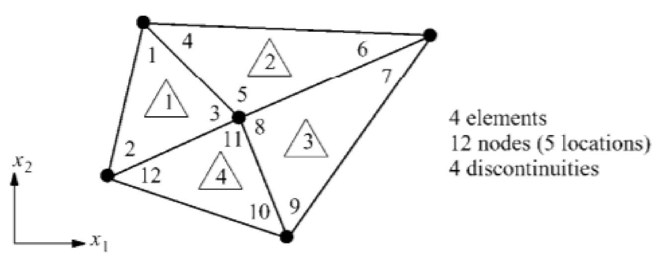
24] in order to meet all requirements for the stability analysis, and the method uses three types of the elements under the conditions of plane strain as shown in
Figure 1. It has been documented that the stress field for each of these elements is assumed to vary linearly.
On the other hand, the literature [
19] reveals that the first formulation for the upper bound theorem was developed in 1972, with the purpose of analyzing the plate problems, further modifications were then introduced thereafter by scholars such as Bottero et al. [
20], Sloan [
22], and Yu et al. [
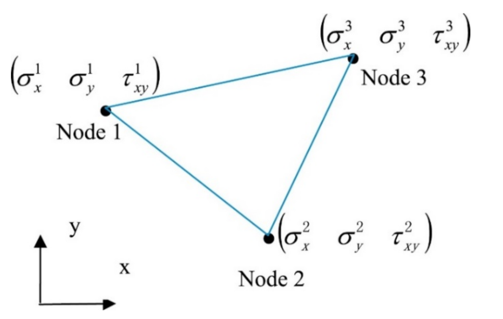
25], to incorporate velocity discontinuities in a plane strain of limit analysis. Although there has been some improvement, the upper bound formulations did not have a large number of discontinuities in the velocity field, therefore, Sloan and Kleeman [
26] strived to address the problem in the formulation of the upper bounds, which is the recent bound used in the current study. An example of the constant-strain triangular element used in the upper bound analysis is shown in
Figure 2.
1.2. Brief Discussion on Literature
Although there have been several improvements on the LEMs in predicting the stability of the slope, the method still presents some limitations as stated within the introduction section. Furthermore, the use of LEMs has gained momentum despite their accuracy error. One may say their simplicity increases their use in the industry, yet there is no accurate predicting chart to benchmark the LEMs solutions, though the SRF method is preferred by few engineers due to its complexity. The recent study is intended to identify the error accuracy of LEMs benchmarked with lower and upper bound limit analysis methods. It is anticipated that the error accuracy chart will give freedom to those engineers who still prefer LEMs over any other method; the authors will be able to benchmark their solutions. Indeed, six common types of soil slope material were chosen to identify the accuracy per material of the slope; however, several case studies also increase the confidence of the outcome of the study.
2. Materials and Methods
The material and methods section of the paper is divided into two sections. The first section documents the limit equilibrium method applied in this study, and the mathematical formulation of each method is documented followed by the description of the procedures followed when simulating LEM solution using a computer code called SLIDEs 2D. In the second section of governed by limit equilibrium method, a brief description of the strength reduction factor method of limit analysis is documented followed by its mathematical formulations in terms of governing equations, lower and upper bounds principles, bounds and duality formulations, and lastly the procedure for a computer code called Optum G2 is briefly documented.
2.1. Limit Equilibrium
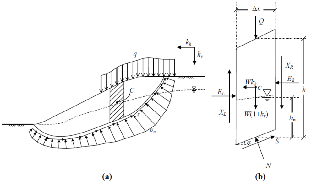
The limit equilibrium approach assumes that a slope is stable when any free-body inside the soil medium is at rest; this implies that the static equilibrium conditions are satisfied. Based on this assumption, LEMs cannot yield a direct measure of system reliability; instead, they analyze multiple paths within the soil profile to determine the critical slip surface. For the given soil slopes surfaces, the stability level was quantified using a constant name called Factor of Safety (FOS), which is the ratio between the available soil shear strength and the equilibrium shear stress at the slip surface. In this regard, the FOS of the soil slopes is expressed by Equations (1) and (2). Equations (1) and (2) were formulated considering the generic slip surface as shown in
Figure 3, the mobilized shear strength was determined based on the inertial forces and external loads as well as base reactions. Depending on the type of problem and the accuracy of results required, this approach uses different analysis methods such as Ordinary method, Bishop Simplified, Gle/Morgenstern–Price, Janbu Simplified, and Janbu Corrected, Spencer and Corp of Engineer number one, and Corp of Engineer number two. A detailed description of the formulation of the methods is documented below since all these methods were used in this study.
where
τ: peak shear stress,
: equilibrium shear stress,
: normal stress,
and
: soil cohesion and friction angle (i.e., subscript “
” denotes the mobilized parameters).
2.1.1. Ordinary Method
The Ordinary method (OM) has been well known to satisfy the moment equilibrium for a circular slip surface [
27], while neglecting both the interslice normal (E) and the shear forces (T). The common advantage of this method is its simplicity in solving the safety factor (FOS), because its equation does not require interaction processes. Furthermore, the method is considered inaccurate for a flat slope with high pore pressure. As already indicated, the FoS of the method is based on moment equilibrium, therefore, the FoS equations are computed as follows [
7,
27]:
where:
,
c′,
φ′,
and
are the inclination of slip surface at the middle of slice, cohesion, friction angle, pore pressure, and slice base length, respectively.
2.1.2. Bishop’s Simplified
The Bishop’s Simplified method (BSM) is very popular in geotechnical engineering, the method is considered accurate for only circular slip surfaces [
27,
28]. Nonetheless, the method also satisfies vertical equilibrium and the overall moment equilibrium. Furthermore, the method assumes that side forces on slices are horizontal. The method is given by the following equation;
where
.
Lastly, the FOS is determined through the iteration processes [
28].
2.1.3. Janbu’s Simplified
Janbu’s Simplified method (JSM) is considered to be a force equilibrium method and it is applicable to any shape of the slip surface. The method assumes that side forces are horizontal (same for all slices) and safety factors are usually lower as compared to another method that calculated safety factors by satisfying all conditions of equilibrium. The safety factor equation that governs this method is shown below [
28].
where
.
2.1.4. Janbu’s Generalised
Janbu’s Generalised method (JGM) satisfies all the conditions of equilibrium, it is also applicable to any shape of the slip surface. The method assumes the heights of side forces above the base of the slice (usually varied from slice to slice). It is also considered to be the accurate method and the one that is applied most frequently in numerical convergence problems. The FOS equation that governs this method is shown below [
28].
where,
is FoS E,
re forces.
2.1.5. Corps of Engineers
Corps of Engineers method (CEM) is an accurate method of force equilibrium, and it is also applicable to any shape of the slip surface. The method assumes that the side force inclination is equal to the inclination of the shape (same from slice to slice). The Factor of Safety is often considered higher than when calculated using another method that satisfies all equilibrium conditions. The FOS equation that governs this method is shown below [
28].
where, λ is scale factor of the assumed function,
is the interslice forces,
is the FOS.
2.1.6. Morgenstern-Price
Morgenstern–Price method (MPM) is an accurate method of force equilibrium, and it is also applicable to any shape of the slip surface. The method assumes that the inclination of the side force follows a prescribed pattern, so-called
f(
); the side force inclination can be the same or vary for every slice and the side force inclination is calculated in the process of the solution to ensure that the equilibrium conditions are satisfied. The FOS equation that governs this method is shown below [
28].
where,
is the interslice force function that varies continuously along the slip surface, λ is the scale factor of the assumed function,
is the interslice forces,
is the FOS.
2.1.7. Spencer’s Method
Spencer’s method (SM) is an accurate method of force equilibrium, and it is also applicable to any shape of the slip surface. The method assumes that the inclination of the side force is the same for every slice and the side force inclination is calculated in the process of the solution to ensure that the equilibrium conditions and satisfied. The FOS equation that governs this method is shown below [
28].
All mentioned above governing equations of the limit equilibrium methods were applied in a Rocscience code called SLIDEs 2D to simulate the stability number of the slope. The procedure for the computer code is documented below.
2.1.8. SLIDES Computer Code Procedures
The computational procedures for SLIDEs are well explained in several studies such as those of Sengani and Mulenga [
29,
30]. The SLIDEs were utilized to estimate the FOS of the slopes in six scenarios; however, the code has the ability to use various LEMs at a time. In terms of model building, it starts with the creation of a new project. Similar to other modeling platforms, the new project required the delimitation of the model limitation in XY coordinates. For that, various X and Y coordinates defining the region were entered. The ultimate goal of this step was to draw the model of the region. Upon generating the boundaries of the model, the actual initial conditions of the simulation are defined next for the project. Inputs such as the statistics associated with groundwater conditions, the computational methods, and the failure directions are captured.
2.2. Limit Analysis
The limit analysis of this study is performed using the so-called strength reduction factor (SRF) or strength reduction method (SRM). The SRM is mostly based on the finite element method (FEM) or finite difference method (FDM) to overcome the limitations presented by limit equilibrium methods. The SRM method was firstly proposed by Zienkiewicz et al. (1975) with the purpose of analyzing slope stability; however, the method has gained more interest with many scholars [
31,
32,
33,
34,
35] striving to improve the method. It has been observed that several scholars [
36,
37] have confirmed that SRM solutions are more accurate and can be closely related to the LEM solutions; this allows us to use the SRM as a benchmark method in evaluating the accuracy of the LEM method.
In the strength reduction method, the Factor of Safety (FOS) is defined as the ratio between the actual shear strength and the reduced shear strength for the fault, joints, and intact rock when the slope arrives at a critical state. When implementing the strength reduction procedure, the reduced shear strength parameters, cohesive force
and the fiction angle
are obtained by the following (see Equation (11)):
As already stated that the SRMs are based on FEM, therefore, these methods have governing equations followed by their mathematical formulations in terms of the bound solutions (lower and upper) as well as the duality and bounds equations of the model. A detailed description of the mathematical formulation of the used SRM is documented below.
2.2.1. Governing Equations
Governing equations defining the mathematical implementation of the FEM model of a solid system are encapsulated in Equations (12)–(17). Assuming an infinitesimal deformation is to be simulated, the equations can be expressed as follows [
38]
Equilibrium and static boundary conditions of the model:
where
are the stresses,
are the body forces stemming for example from self-weight, and V is the domain under consideration.
Meanwhile, the yield conditions of the model are as follows:
Since the current situation is dealing with strain problems, therefore, associate flow rules or strain-displacement compatibility has to be incorporated as follows;
where
is the plastic multiplier that satisfies the complementarity conditions.
Therefore, the scaling applied with respect to the rate of work done by the reference tractions
t as indicated above, in short, the scaling equation is denoted as follows;
where
is taken as the exact velocity,
t is traction vector
Lastly, the complementarity conditions of the model are, therefore, incorporated as follows:
Nevertheless, a detailed description of the model in terms of lower bound principle, upper bound principles, bounds are documented below.
2.2.2. Lower Bound Principle
In terms of the lower bound principles, the principle ensures that the strain-softening aligns with the governing equation of the limit analysis of the finite element. However, the kinematic quantities, which are absent from the governing equations, appear as Lagrange multipliers when solving the problem. The main strength of the lower bound principle is that it allows for a lower bound on the exact collapse multiplier to be computed, through constructing a stress field that satisfies the constraints without necessarily being optimal [
39].
2.2.3. Upper Bound Principle
As already stated, the problem at hand incorporates the kinematic quantities that the LEMs do not have the ability to handle; therefore, the upper bound is intended to incorporate the compatible velocity field that satisfies the flow rule. A similar flow rule cannot be activated using the LEMs, therefore, this upper bound is indeed critical. In order to achieve that, the rate of work done by the reference tractions is scaled to unity and the objective function, which comprises the internal rate of work minus the contribution from the constant body forces, is then the collapse multiplier sought. The upper bound principles are denoted in Equation (19).
2.2.4. Bounds
The bounds are a critical part of the numerical simulation because this stage is used to verify the lower and upper bound principles to ensure that the bounds furnish with a collapse multiplier. Therefore, the stress field is considered first, to ensure that they satisfy the yield condition and the equilibrium conditions as well as the boundary conditions. Such expression on how the bound is performed is documented by Equation (20).
2.2.5. Optum G2 Computer Code Procedures
The model procedure followed in Optum G2 is readily available on the Optum Computational Engineering website under Optum G2 analysis and examples. In summary, the procedure followed includes the project definition (project file dialog, slope parameters dialog, model layout), building the model in terms of model layers, input properties of the material, and model setting. After processing the provided information in the model, the results of the model are then presented in terms of SRF, gravity multiplier, though the current study is interested in SRF analysis only. Furthermore, the model can also provide results on displacement, stress, the strain among other aspects such as yielding function and dissipation. As already stated, the model build was varied based on the material properties the case is interested in and the material properties of each case are given in
Table 1 below.
3. Results
The results of this paper are divided into two sections, the first section presents numerical simulation results in a homogenous road slope using the Mohr–Coulomb model. In this section, several examples on the prediction of Factor of Safety or Strength Reduction Factor using both limit equilibrium (SLIDEs) and limit analysis (Optum G2) are presented. Indeed, a detail comparing the accuracy of the LEMs in predicting the stability of the slope is well presented, the presentation of these results also incorporates the overestimation of FOS by several LEMs compared with the SRF stability number predicted. As already stated, several examples were used to quantify the accuracy prediction of slope stability using LEMs benchmarking with a limit analysis approach, a homogenous road slope with loose sand, medium sand, dense sand, soft clay, firm clay, and stiff clay mechanical properties are used to conduct the investigations. However, the slope solid material properties differ in terms of stiffness, strength, flow rule, unit weight, and hydraulic conditions. As such, a clear distinction of the accurate prediction of slope stability of the road slope in strain-softening has been documented.
The second section of the results document a classification chart in terms of accurate prediction of slope stability among the LEMs. The chart classifies LEMs accuracy in terms of their rate of overestimating the stability of the slope, with the most accurate methods considered to be those with less percentage of overestimating the stability of the slope. The chart was based on the previous section and benchmarked with the limit analysis results.
3.1. Stability Analysis of a Homogenous Road Embankment Slope
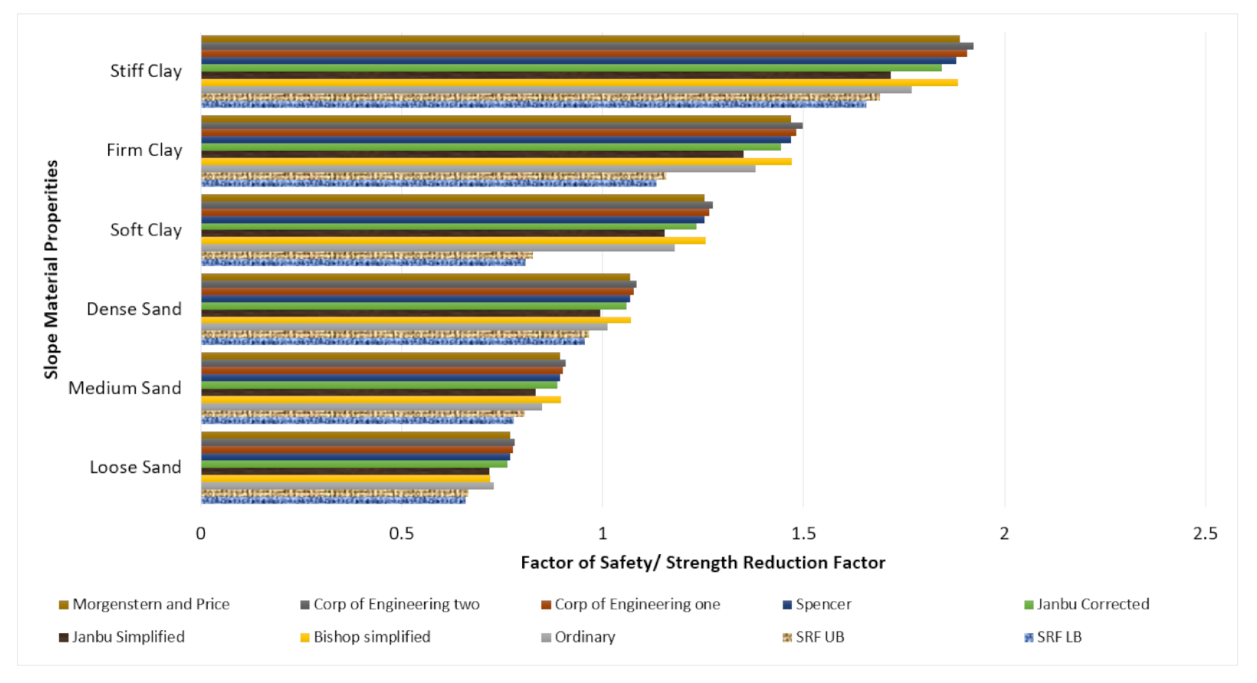
The results of homogenous slope stability calculations using the rigorous upper and lower bound methods of limit analysis and the limit equilibrium method (Ordinary, Bishop, Gle/Morgenstern–Price, Janbu Simplified, and Janbu Corrected, Spencer, and Corp of Engineer number one, and Corp of Engineer number two) are presented in
Figure 4, for slope with homogenous loose sand, medium sand, dense sand, soft clay, firm clay, and stiff clay, respectively. The limit analysis results are plotted in terms of Strength Reduction Factor for both lower and the upper bounds; however, the simulation also included the slope total displacement though it is not of interest. The solutions from limit equilibrium computer code SLIDEs 2D are presented in terms of Factor of Safety for all stated methods. In both computer codes, it is assumed that the material gain strength with depth. Similar to other studies such as Yu et al. [
40], to account for the effect of increasing strength with depth, the results are always presented in terms of stability number (SRF or FOS) against the dimensionless parameters. For each homogenous slope, the stiffness, strength (cohesion, friction angles) unit weight (dry and saturated soil), and hydraulic conditions differ greatly. Furthermore, the geometry of the slope was kept constant throughout different case studies given, details of each case study are outlined below.
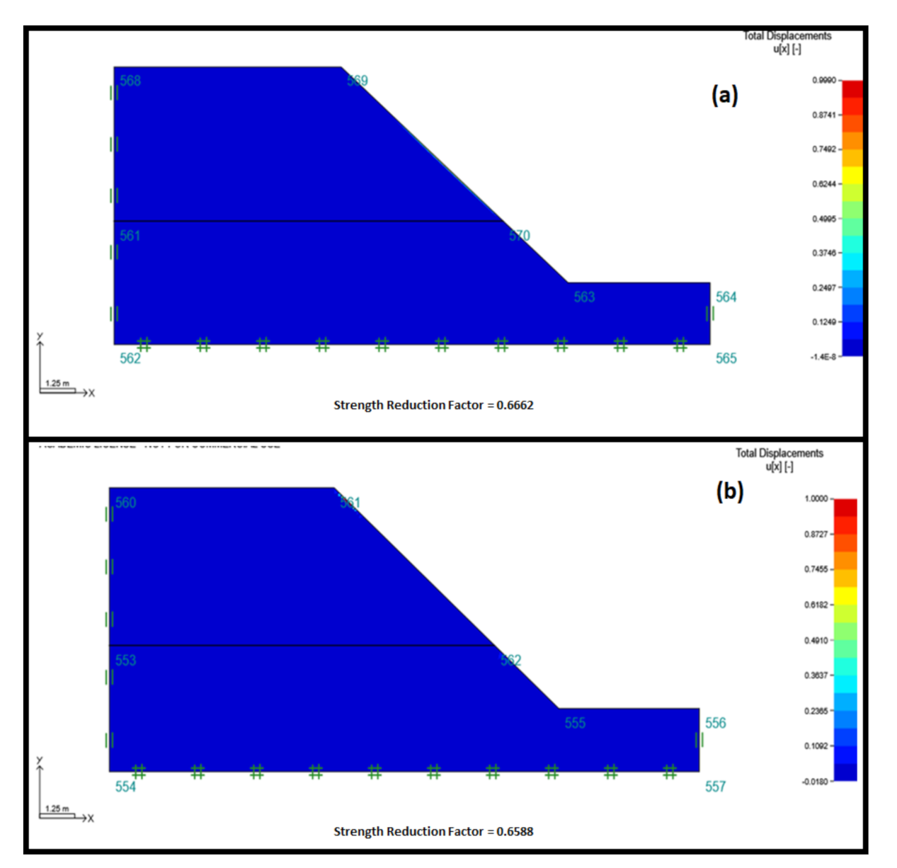
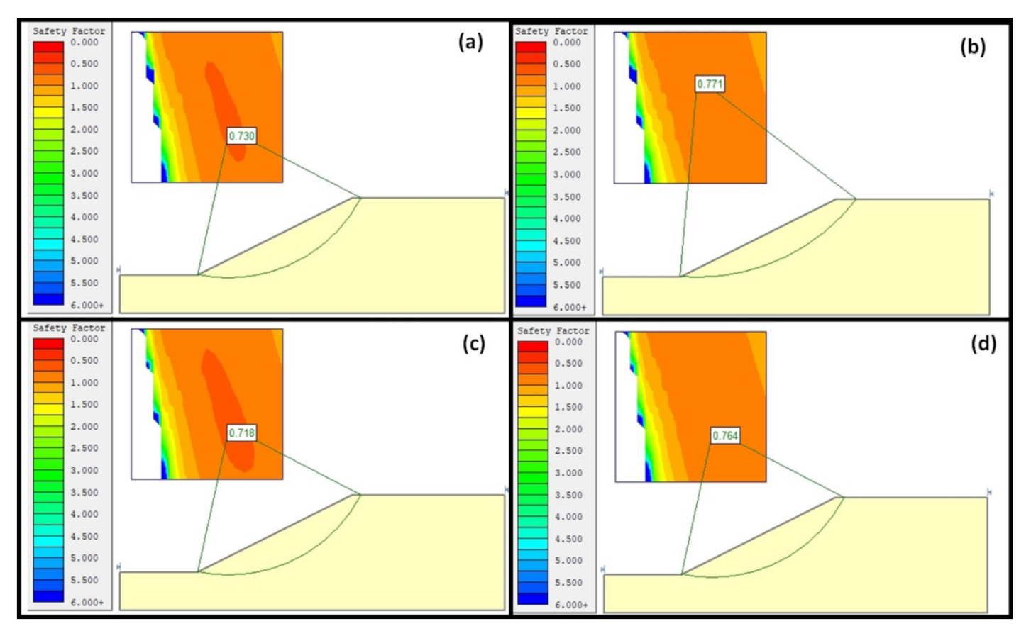
3.1.1. Road Embankment Slope with Loose Sand
A soil slope with a slope angle of 45° is selected as a case study shown in
Figure 5,
Figure 6 and
Figure 7. In the slope, loose sand with a friction angle of 13°, the cohesion of 3 kPa, and unit weight of 14 kN/m
3, and other input parameters as shown in
Table 1, were taken into consideration. Both rigorous lower and upper bounds limit analysis and limit equilibrium methods were used to perform the analysis through separate numerical codes and were implemented as stated by the methodology section. The results of the limit analysis have shown that the slope is expected to be unstable considering the effect of an increase in strength of material with a depth of slope. Furthermore, the lower bound solution estimated the SRF of 0.6588 while the upper bound solution was about 0.666 SRF. On the other hand, the limit equilibrium method solutions were ranging from 0.718 FOS to 0.776 FOS. For all the cases considered (see
Figure 6 and
Figure 7), it has been denoted that the exact solutions are bracketed within 8 to 17% of error accuracy. This implies that among the limit equilibrium methods, none of them were able to provide the exact solutions as compared to the rigorous lower or upper bound solutions; however, the LEMs solutions were denoted to be closely related to those of the upper bound solutions. Indeed, this type of result has been demonstrated by previous scholars such as those of Yu et al. [
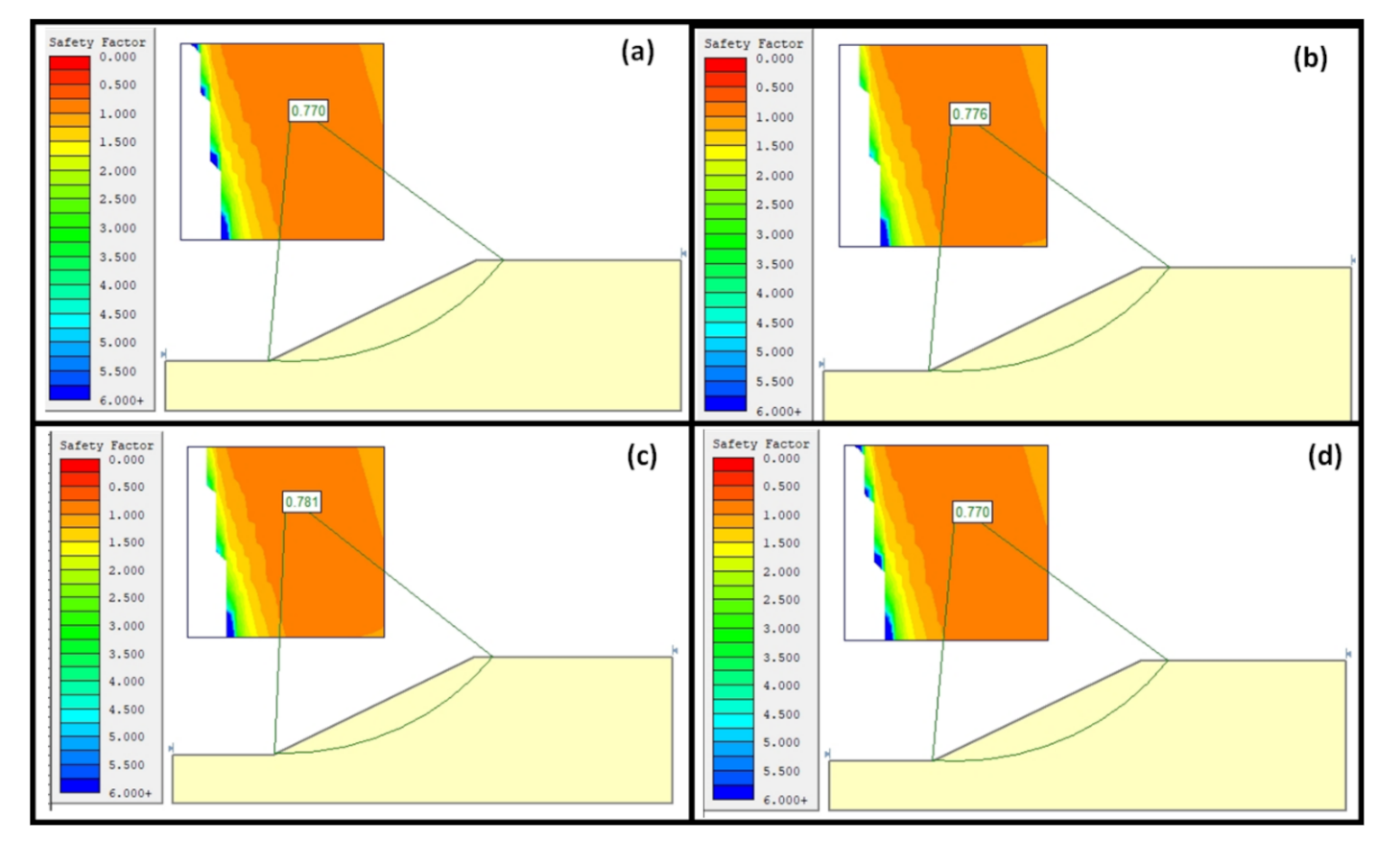
40]. Meanwhile, the Corp of Engineer number two was found to produce the highest accuracy error in predicting the stability number. Though several scholars assumed that the LEMs produce similar results with the limit analysis based on the predicted SRF and FOS number without considering the calculation of error accuracy or benchmarking the two methods, the outcome of this analysis demonstrated different views within those studies, such as Renani and Martin [
1]. One may denote that, previous studies such as those of Renani and Martin did not consider exact solutions but closely related solutions and by so doing the author came to the conclusion that the solutions of LEMs and rigorous upper bound solutions are similar.
It was also observed that the Bishop Simplified method of limit equilibrium also produces a stability number that has a good agreement with the upper bound solutions of the limit analysis. The method has produced a stability number with an accuracy error of about 9%, which is acceptable in the industry. That being said, the Bishop Simplified method accuracy error solution was closely related to that of the Janbu Simplified method with just a 1% difference. Furthermore, another method including Spencer, Morgenstern–Price, and Corp of Engineering produced an accuracy error above 10% but less than 20%. In summary, all the LEMs produce the stability number that is closely related to that of the upper bound solutions but the stability numbers are not the same. Further case studies are discussed below to solidify the outcome.
3.1.2. Road Embankment Slope with Medium Sand
Similar soil slope profiles were considered in this case as well, as shown in
Figure 7,
Figure 8 and
Figure 9. In the slope, medium sand with a friction angle of 15°, the cohesion of 4 kPa, and unit weight of 16 kN/m
3, and other input parameters as shown in
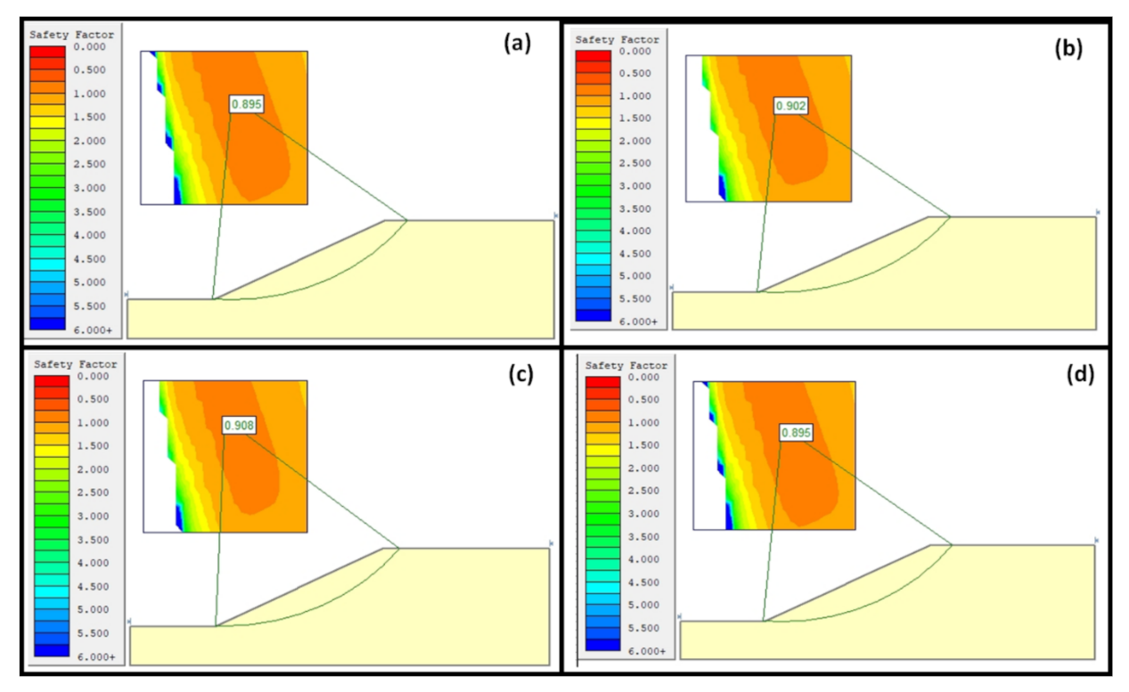
Table 1, were taken into consideration. Both rigorous lower and upper bounds limit analysis and limit equilibrium methods were used to perform the analysis. The results of the limit analysis have shown that the slope is expected to be unstable. The lower bound solution estimated the SRF of 0.7782 while the upper bound solution was about O.8068 SRF. On the other hand, the limit equilibrium method solutions (FOS) ranged from 0.834 to 0.908. For all the cases considered (see
Figure 8 and
Figure 10), it was denoted that the exact solutions are bracketed within 3 to 13% of error accuracy. This implies the limit equilibrium method is still considered to produce reasonable solutions in medium sand; however, the Janbu and Ordinary methods were found to produce very small accuracy errors ranging between 3 and 5%, which is still within the acceptable error accuracy.
On the other hand, Corp Engineering two was also observed to produce the highest error of accuracy but in this case, the error was just about 10%. This gives an impression that almost all limit equilibrium methods can produce solutions that are in good agreement with the upper solutions in medium sand. Similar observation as the previous case the spencer and Morgenstern–Price methods produced similar stability.
3.1.3. Road Embankment Slope with Dense Sand
A soil slope with a slope angle of 45° is selected as a case study shown in
Figure 5,
Figure 6 and
Figure 7. In the slope, dense sand with a friction angle of 17°, the cohesion of 4 kPa, and unit weight of 16 kN/m
3, and other input parameters as shown in
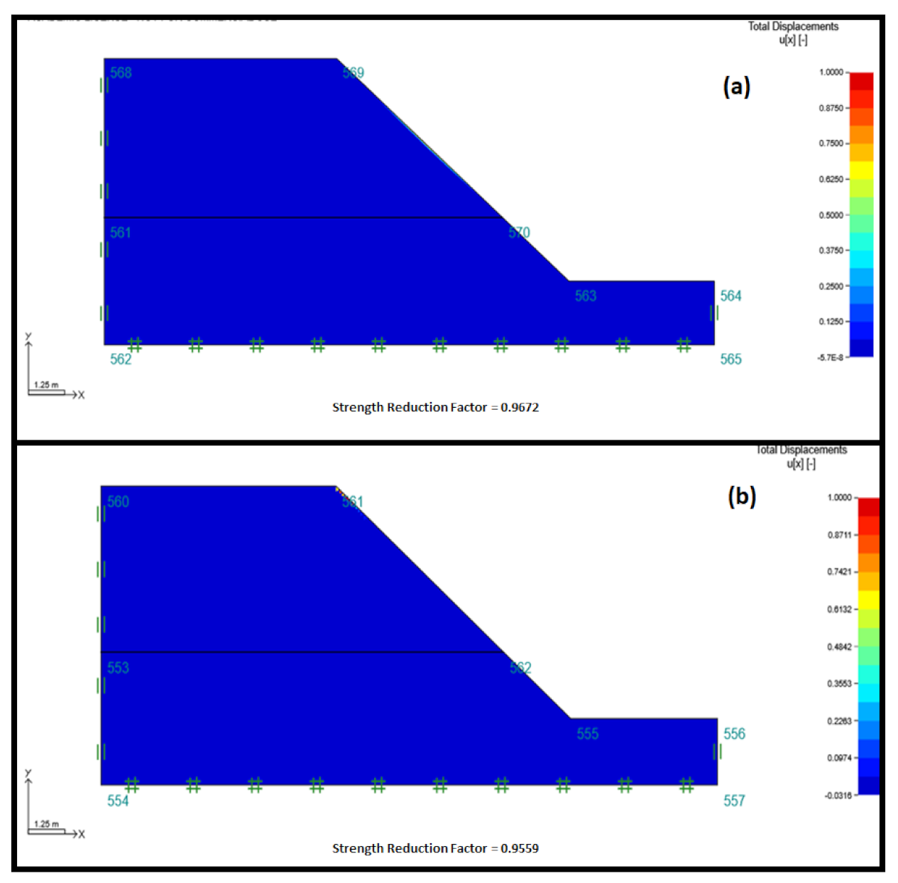
Table 1, were taken into consideration. Both rigorous lower and upper bounds limit analysis and limit equilibrium methods were used to perform the analysis through separate numerical codes were implemented as stated by the methodology section. The results of the limit analysis have shown that the slope is expected to be unstable considering the effect of the increase in strength of material with a depth of slope.
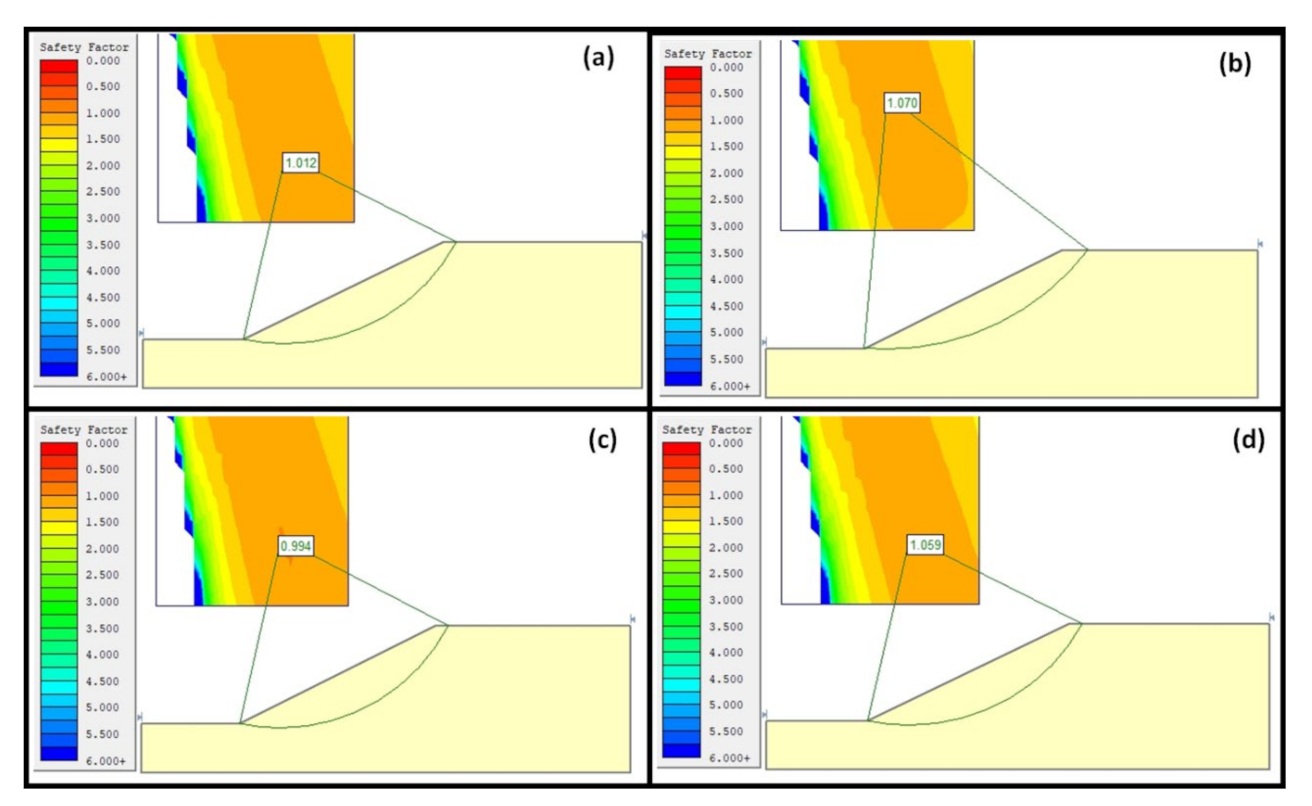
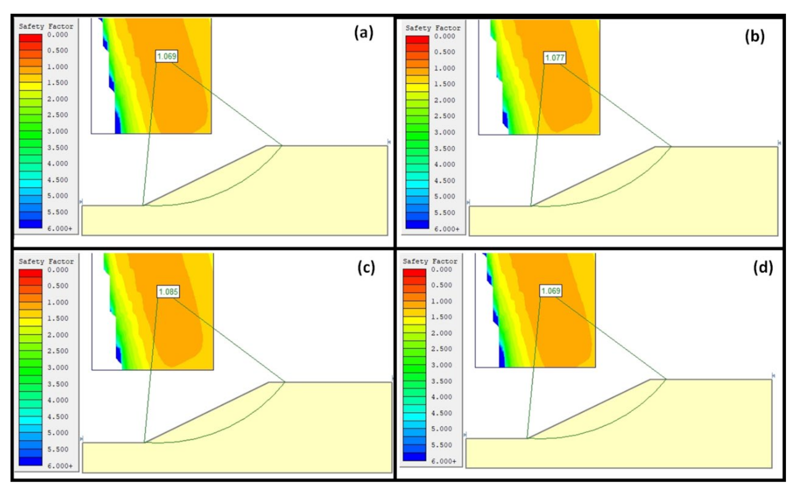
Furthermore, the lower bound solution estimated the SRF of 0.9559 while the upper bound solution was about 0.9672 SRF. On the other hand, the limit equilibrium method solutions were ranging from 0.994 FOS to 1.085 FOS. For all the cases considered (see
Figure 11,
Figure 12 and
Figure 13), it has been denoted that the exact solutions are bracketed within 8 to 17% of error accuracy. In this case, the limit equilibrium method produces two scenarios wherein Janbu Simplified classifies the slope as unstable and the solutions are closely related to those of the upper solutions. On the other scenario the rest of the method classified the slope as stable, this implies that most of the LEMs have overestimated the stability of the slope.
3.1.4. Road Embankment Slope with Soft Clay
A soil slope with a slope angle of 45
0 was selected as a case study shown in
Figure 14,
Figure 15 and
Figure 16. In the slope, a soft clay with a friction angle of 18
0, the cohesion of 9 kPa, and unit weight of 19 kN/m
3, and other input parameters as shown in
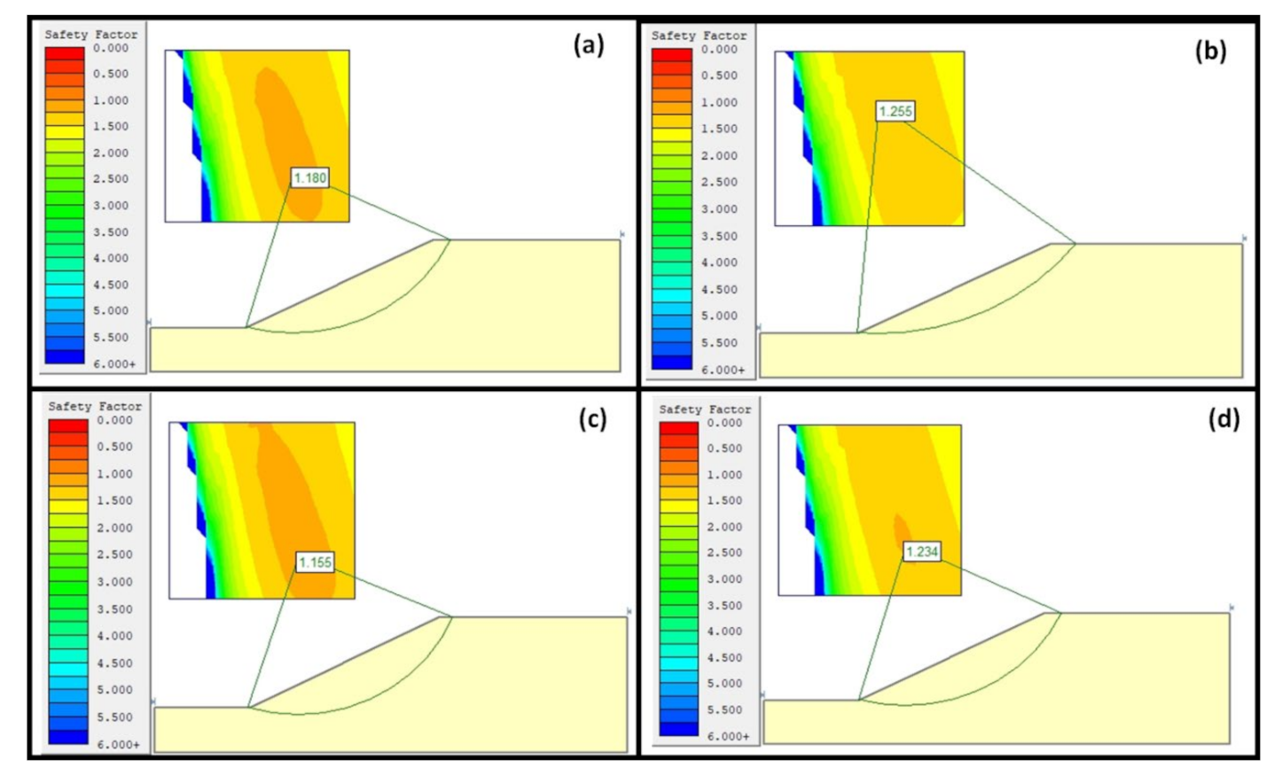
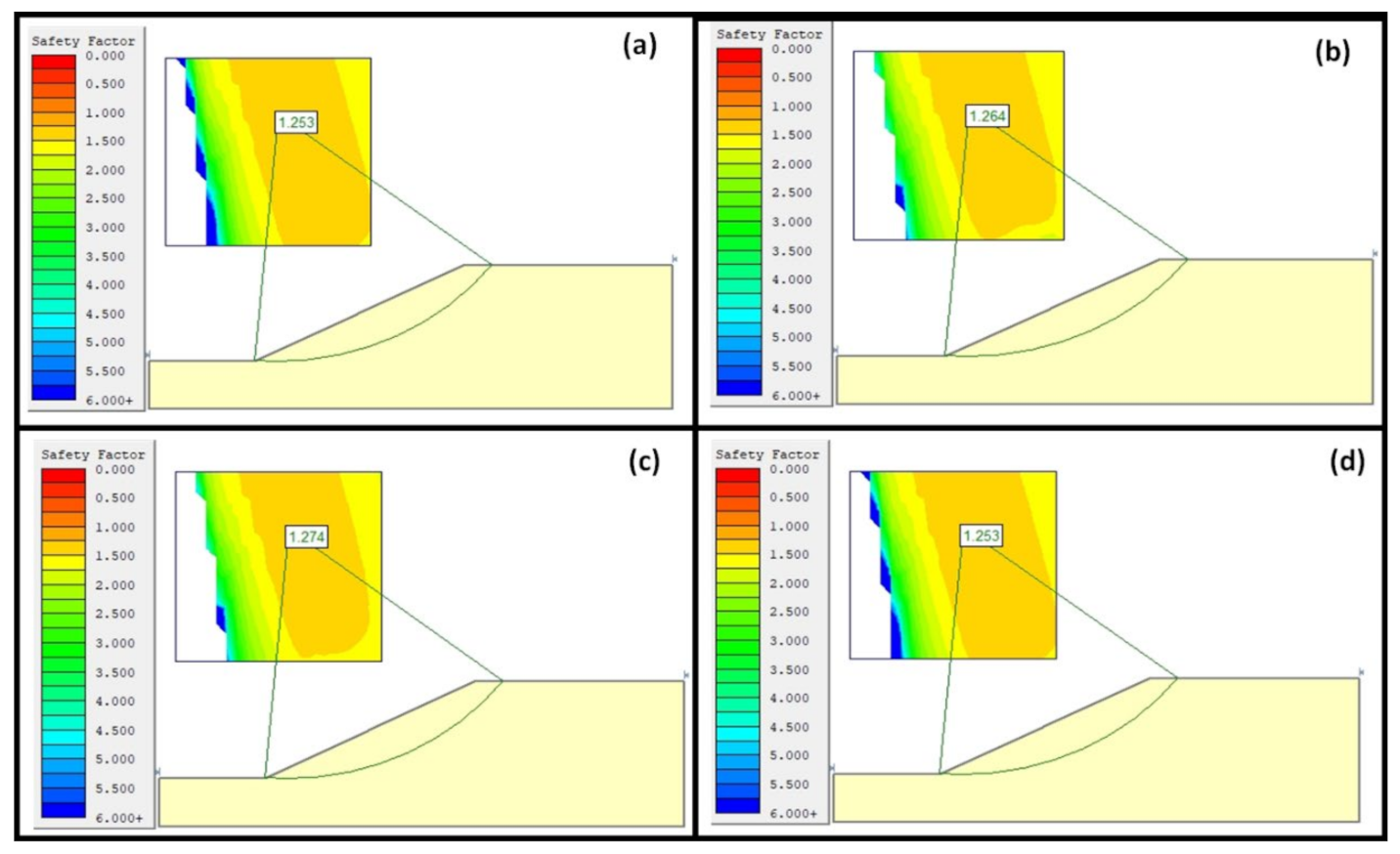
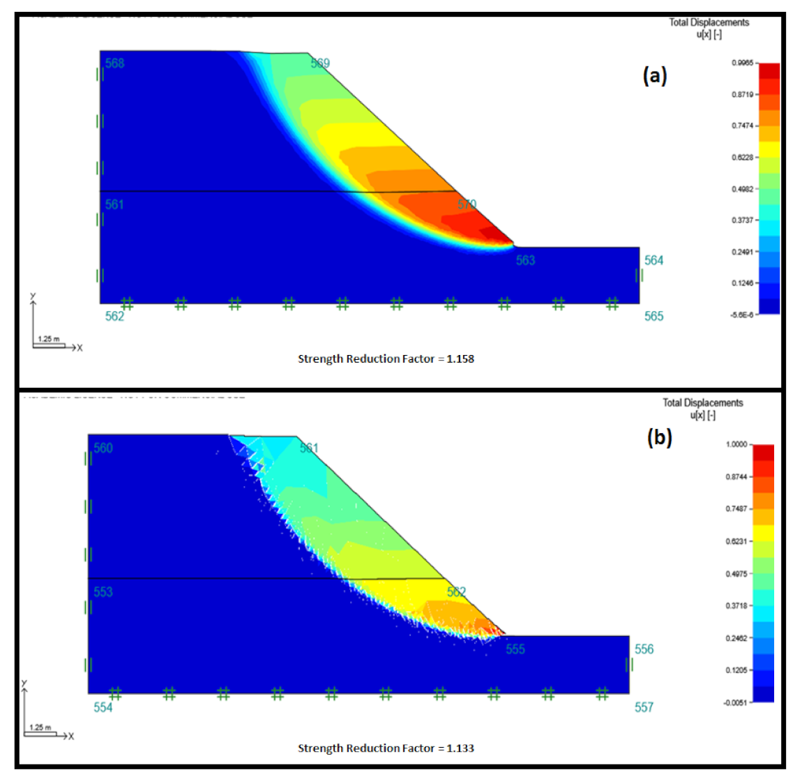
Table 1, were taken into consideration. Both rigorous lower and upper bounds limit analysis and limit equilibrium methods were used to perform the analysis. The results of the limit analysis have shown that the slope is expected to be unstable using the rigorous lower and upper bound solutions with the SRF of 0.8257 and 0.8079 for upper and lower, respectively. Meanwhile, the limit equilibrium method solutions estimated a stable slope with FOS ranging from 1.155 to 1.274 (see the simulation results in
Figure 14,
Figure 15 and
Figure 16).
For all the cases considered (see
Figure 14 and
Figure 16), it has been denoted that the exact solutions are bracketed within 40 to 54% of error accuracy. This implies among the limit equilibrium method, none of them were able to provide the exact solutions as compared to the rigorous lower or upper bound solutions. In this regard, all methods were found to overestimate the stability number of the slope. This implies that LEMs are not best to use in soft clay soil slope due to the high accuracy error produced by the methods.
It was also observed that this material behaves differently among others, which demonstrates that though the slope maybe consists of soil, the properties of the soil matter in order to estimate the stability number accurately. One may argue that such abnormality observed could be due to the fact that the limit equilibrium formulations suffer from including stress and deformation of the material [
1], meanwhile, the failure surface is predefined by engineers, which results in predicting such high stability number.
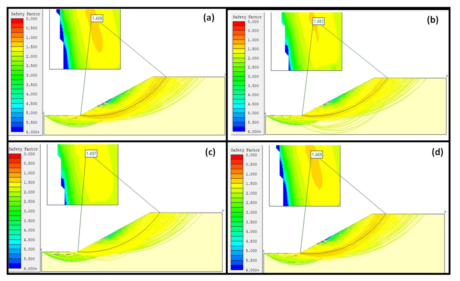
3.1.5. Road Embankment Slope with Firm Clay
A soil slope with a slope angle of 45° is selected as a case study shown in
Figure 17,
Figure 18 and
Figure 19. In the slope, firm clay and with friction angle of 13°, the cohesion of 3 kPa, and unit weight of 14 kN/m
3, and other input parameters as shown in
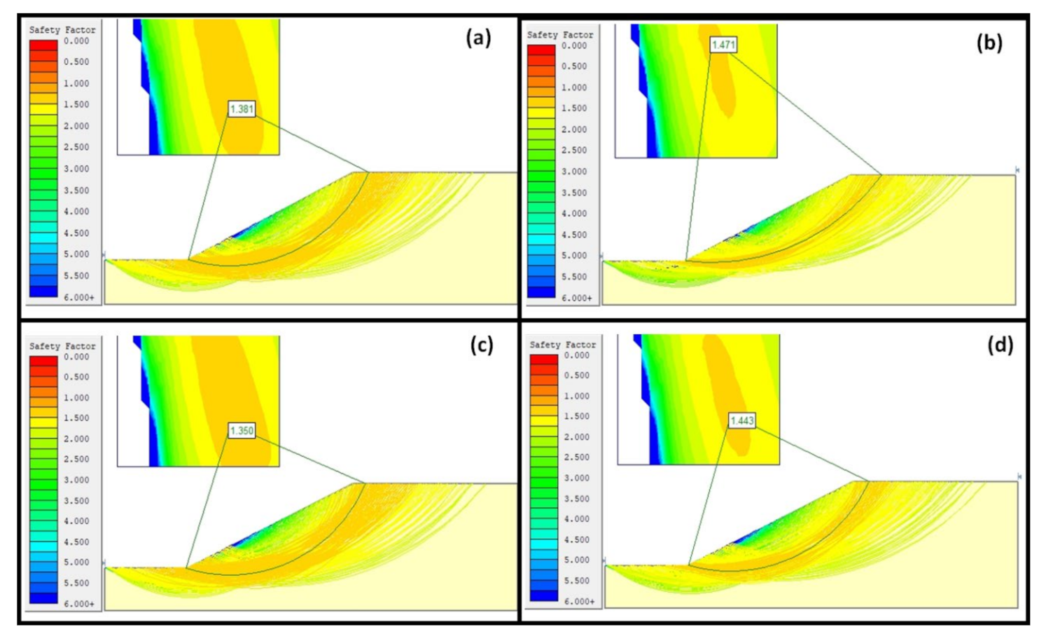
Table 1, were taken into consideration. Both rigorous lower and upper bounds limit analysis and limit equilibrium methods were used to perform the analysis through separate numerical codes and were implemented as stated by the methodology section. The results of the limit analysis have shown that the slope is expected to be unstable considering the effect of the increase in strength of material with a depth of slope. Furthermore, the lower bound solution estimated the SRF of 0.6588 while the upper bound solution was about 0.666 SRF. On the other hand, the limit equilibrium method solutions ranged from 1.350 to 1.497. For all the cases considered (see
Figure 17 and
Figure 19), it has been denoted that the exact solutions are bracketed within 17 to 29% of error accuracy. This implies among the limit equilibrium method, none of them were able to provide the exact solutions as compared to the rigorous lower or upper bound solutions.
It was also observed that the result also shows that the Janbu Simplified limit equilibrium method had much closely related solution to those of the upper bound solutions as compared to other LEMs; however, the method produces about 17% error accuracy as compared to the benchmarking rigorous upper bound solutions of limit analysis. This implies that none of the limit equilibrium methods have an accuracy error below the acceptable industry, therefore, LEMs are not recommended in analyzing soil slope with firm clay.
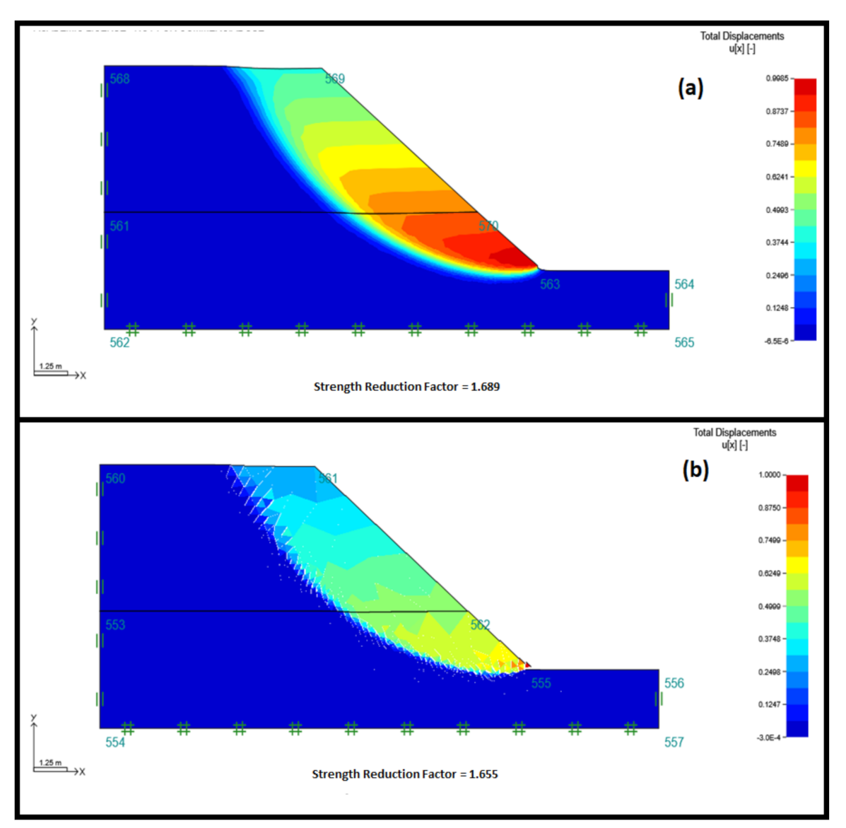
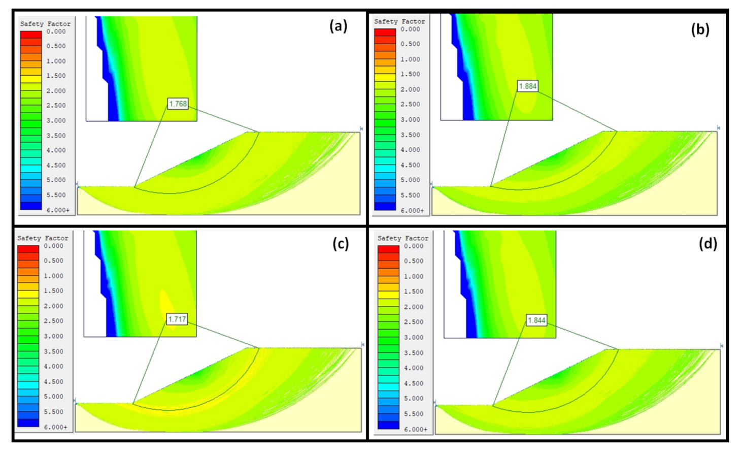
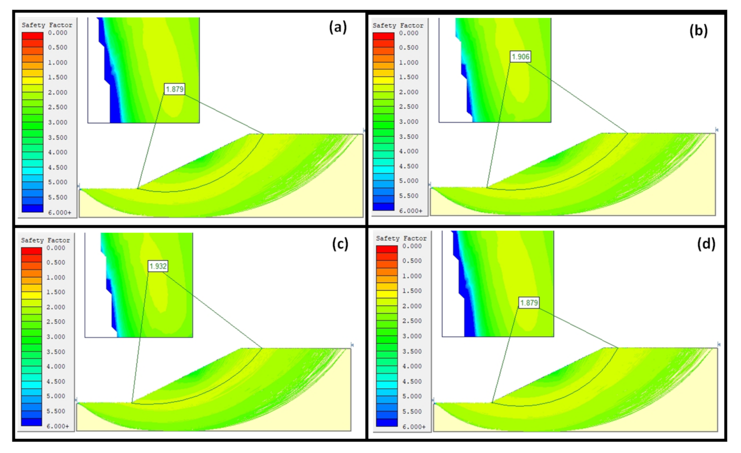
3.1.6. Road Embankment Slope with Stiff Clay
A soil slope with a slope angle of 45° is selected as well as demonstrated in
Figure 20,
Figure 21 and
Figure 22. In the slope, a stiff clay with a friction angle of 22°, the cohesion of 20 kPa, and unit weight of 21 kN/m
3, and other input parameters as shown in
Table 1, were taken into consideration. Both rigorous lower and upper bounds limit analysis and limit equilibrium methods were used to perform the analysis through separate numerical codes and (SLIDEs and Optum G2) were implemented. The results of the Limit Analysis have shown that the slope is expected to be stable. Furthermore, the lower bound solutions estimated the SRF of 1.655 while the upper bound solutions were about 1.689 SRF, while the limit equilibrium method solutions ranged from 1.717 FOS to 1.932 FOS. For all the cases considered (see
Figure 20 and
Figure 22), it has been denoted that the exact solutions are bracketed within 5 to 14% of error accuracy. This implies among the limit equilibrium method, none of them were able to provide the exact solutions as compared to the rigorous lower or upper bound solutions; however, the LEMs solutions were denoted to be closely related to those of the upper bound solutions.
It was observed that among other cases considered, limit equilibrium methods perform much better in stiff clay, in summary, the error accuracy produced by Janbu Simplified was about 2%, which is almost the same as the exact solutions of the upper bound solutions. This implies that though the LEMs are known to produce less accurate solutions, the method produces different accuracy errors based on the material dealt with. In this study, it may be deduced that almost all LEMs used for the study were within the required acceptable accuracy error of the industry. Furthermore, the Ordinary method was also found to be the second-best method in terms of producing low error accuracy, and results show that Ordinary and Janbu Simplified can be recommended as reasonable methods to use in order to acquire close related solutions to those of upper bound solutions of limit analysis. On the other hand, the Corp Engineering Two method was still found to be the last method to produce closely related solutions to those of upper bounds, but their solutions were still less than 15%.
These results bring a similar argument that it cannot be assumed that LEMs produce similar results though the solutions produced by two methods are not exact. In simple terms, the results of this paper demonstrate some disagreement with previous studies such as Cheng et al. [
36], Renani and Martin [
1]; however, the disagreement lies along the lines of assuming that no exact solutions are similar without considering the error accuracy generated by very small differences in solutions. Indeed, the behavior of the material in terms of how they respond to each method may have been partial captured, some of the studies that strive to capture the response of different soil material behavior on the slope are those of Bjerrum [
41], Skemton [
42], Hettler and Vardoulakis [
43], but still there is no specification of error accuracy of the LEMs. A section below is, therefore, intended to develop an accuracy classification chart of LEMs in predicting stability numbers based on the benchmarking discussed in this paper.
3.2. Accuracy Classification Chart of Limit Equilibrium Method in Predicting the Stability of the Homogenous Slope
For all the cases considered in the sections above (
Figure 21), it has been observed that in almost all cases, the Janbu Simplified limit equilibrium solutions are found to be in good agreement with the rigorous upper and lower bounds, but close to the limit analysis rigorous solutions of the upper bounds. In all cases, the limit equilibrium results were generally close to those of the upper bound solutions, while the lower bound solutions appeared to be underestimated compared to all the limit equilibrium solutions presented.
In summary, the Janbu Simplified limit equilibrium method produces the most reasonable accurate solutions for the stability of homogenous soil slope whose strength increases with depth. Nevertheless, the Janbu Simplified limit equilibrium method was very accurate (1–7% of overestimated as compared to the rigorous upper bound solutions) in homogenous slope consisting of stiff clay, dense sand, and medium sand. In fact, the method (Janbu Simplified) presented an accuracy error of about 1% when estimating the stability of the slope in stiff clay, these results imply that the method has the ability to produce similar or closely related results to those of the upper rigorous bound solutions of limit analysis. Furthermore, the reliability of the method (Janbu Simplified) was also demonstrated when estimating about 2% accuracy error of the slope stability in dense sand slope, indeed further demonstration was shown when estimating the stability of slope with medium sand, which results in 3% of accuracy error. It was also demonstrated when estimating the stability of the slope with loose sand that the method produces 7% error accuracy, which is still below the acceptable error accuracy of 10%.
In other cases, the method was still denoted to be the most accurate as compared to other limit equilibrium methods; however, in firm clay, loose sand, and soft clay, the predicted stability number was over the acceptable accuracy error percentage, in fact, it was more than 10%. Though the study was focusing on benchmarking the Limit Equilibrium solutions with the limit analysis solution since limit solutions are usually used to overcome the accuracy predicting problem associated with the limit equilibrium solution, one may deduce that the Janbu Simplified solution is in good agreement with the upper bound solution; although in soft clay, the method overestimates by about 40%. In the case of firm clay, the method is just after the acceptable accuracy error (10%) but less than 20%. These results can still be used in cases where rigorous upper and lower bound solutions are not available.
Fair enough, the Janbu Simplified method was not the only method found to produce stability numbers with very low error accuracy, the so-called Ordinary limit equilibrium method was observed to produce very fair solutions or closely related to the rigorous upper bound solution but the solution produces were always greater than those of Janbu Simplified limit equilibrium solutions by about 2–3%. Similar to the Janbu Simplified, the Ordinary limit equilibrium method has produced stability numbers with acceptable error accuracy in almost all cases with the exception of the soft and firm clay. This implies that this method is not in good agreement with the upper bound solutions of limit analysis when predicting the stability of the homogenous slopes subjected to either soft clay or firm clay. Nevertheless, the method has shown its constant prediction throughout the case study given and it was always found to be the second-best in terms of stability number in relationship with the benchmark solutions produced by upper bound solutions.
On the other hand, the Corp of Engineer (2) limit equilibrium solutions was found to overestimate the stability of the homogenous slopes in all given case studies. The overestimation was found to be greater than the acceptable error accuracy in all cases. The accuracy error of this method was also found to be 10 to 13% more than those of Janbu Simplified Limit Equilibrium solutions. Similarly, the method was also denoted to overestimate the stability of the slope in soft clay though the overestimation was about 54%; this result provided a trend in all limit equilibrium solutions that soft clay cannot be accurately predicted despite the method to be used in limit equilibrium.
Another interesting observation was to note that both the Spencer limit equilibrium solutions and the Gle/Morgenstern–Price limit equilibrium solutions were similar throughout. The similarity was observed in each case study given though the method provided reasonable accuracy in other cases and unreasonable accuracy in the other case.
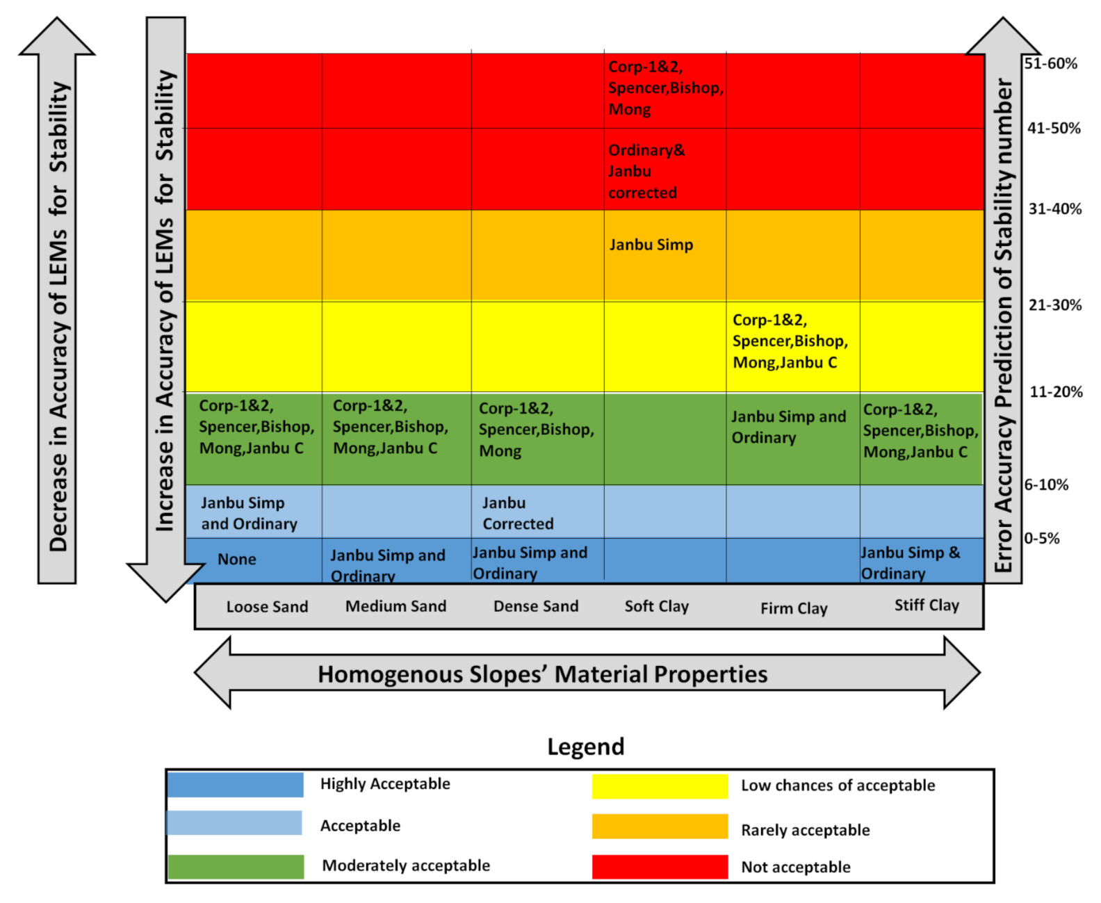
As far as the limit equilibrium method is widely used by engineers and scientists in predicting the stability number of the slope, the concern will always be voiced about the accuracy of these types of solutions. Therefore, a classification chart on accuracy predicting of the limit equilibrium method in a homogenous slope is proposed (see
Figure 23). The chart is based on the results and discussion pointed out above; however, the chart is more concerned with the error accuracy of the limit equilibrium methods in different soil materials, considering the effect of the increase in material strength with depth. Furthermore, the chart can suggest the best limit equilibrium method in estimating the stability of the slope based on material properties. However, the chart is more applicable to those who prefer to use limit equilibrium solutions due to their simplicity.
The chart demonstrates that in the case of loose sand soil slope, the Janbu Simplified and Ordinary methods are preferred to be used due to an acceptable error accuracy ranging between 6 and 10% as compared to the upper bound solutions of limit analysis. Owing to that the chart also denotes that the other six methods may be used but the accuracy error will be ranging from 11 to 20%, in which such error accuracy is not recommended for industry use. In terms of medium sand soil slope, both the Janbu Simplified and the Ordinary are recommended to be used due to their highly acceptable error accuracy, which ranges from 1 to 5%. Meanwhile, others can still be used with caution because of the present accuracy error above the acceptable stand. A similar situation has been observed in dense sand though Janbu is the most accurate method followed by the Ordinary with an error accuracy ranging from 6 to 10%. However, in the case of soft clay, none of the LEMs are recommended due to large error accuracy numbers ranging from 40 to 54%. In firm clay, there are no LEMs that can be used within the acceptable accuracy error, while in stiff clay, the Janbu and the Ordinary are within the acceptable zone.
4. Concluding Remarks
The accuracy of the limit equilibrium methods in terms of estimating the stability number of soil or rock slope has been questioned or called out, yet alternative methods are used rather than addressing the problem at hand. On the other hand, the limit equilibrium methods are preferred over other methods such as limit analysis due to their simplicity. The concern that is often voiced by many engineers and scientists has motivated the present study. Therefore, the present paper strives to address the following objectives: firstly, to identify the most appropriate LEM, in terms of predicting the stability of the slope with a solution that is close to those of SRM/SRF; secondly, to identify which of the bound solutions (lower and upper) is closely related to LEMs solutions in a homogenous soil and rock slope. Several practical examples are used to establish the reliable LEM by comparing the slope stability analysis solutions and the bounding solutions with limit equilibrium methods (eight methods). Six case studies were utilized to establish the above-mentioned objectives and two computer codes (SLIDES-used for LEMs solutions and Optum G2 used for bounding solutions of limit analysis) using finite element formulations were used.
Based on the six case studies considered in this study, it was found that the exact stability solutions produced by the Janbu Simplified and Ordinary methods of limit equilibrium in most cases are bracketed within 2–10% accuracy error as compared to the rigorous upper bound solutions of the limit analysis. However, these conditions of lower accuracy error were noted in loose sand, medium sand, dense sand, and stiff clay soil slope, with the consideration of the effect of the increase in strength of material with depth. It is, therefore, concluded that in cases of the above-mentioned soil slope material, the Janbu Simplified and Ordinary methods of limit equilibrium are the best to implement.
Furthermore, the detailed comparison of the bounding solutions with limit equilibrium methods has also demonstrated that the prediction of stability numbers by Spencer and Morgenstern–Price method are similar throughout, though the methods were not producing closely related solutions to those of upper bound solutions. This implies that the use of these two methods simultaneously is not required since they give similar solutions.
It was also observed that the Corp Engineering number two method of limit equilibrium produced the highest accuracy error percentages throughout the case studies provided; however, its error accuracy was also found to differ from those of the Janbu Simplified bracketed within 10–12%. In simple terms, the method has been found to overestimate the stability number in all cases.
Though the focus was to benchmark the limit equilibrium solutions with the upper and lower bound solutions of limit analysis, all the lower bound solutions were found to be a bit smaller than those of limit equilibrium solutions in all cases. It is, therefore, concluded that the lower bound solutions can be used for designing stable excavation; in other words, the lower bound solutions are closely related to the realistic stability number of the slope as stated by previous scholars such as Yu et al. [
40].
Indeed, a simple accuracy classification chart was developed based on the results of the study. The chart shows various methods of LEMs and their accuracy error percentage per material or soil slope material. It is believed that the chart is useful to engineers who prefer to apply LEMs in classifying the stability of soil slope. Furthermore, the chart also provides room to explore other sophisticated methods that can improve the prediction of error accuracy of the LEMs instability analysis.
Author Contributions
Conceptualization, F.S.; methodology, F.S.; software, F.S. and D.A. validation, F.S. and D.A. formal analysis, F.S. and D.A. investigation, F.S. resources, F.S. and D.A. data curation, F.S. and D.A.; writing—original draft preparation, F.S. writing—review and editing, D.A.; visualization, F.S. and D.A. supervision, D.A.; project administration, F.S.; funding acquisition, F.S., and D.A. All authors have read and agreed to the published version of the manuscript.
Funding
This research was funded by Durban University of Technology and University of Limpopo, grant number 2022-01 and The APC was funded by University of Limpopo.
Institutional Review Board Statement
Not applicable.
Informed Consent Statement
Not applicable.
Data Availability Statement
Not applicable.
Acknowledgments
The authors would like to appreciate the support provided by the Durban University of Technology, Department of Civil Engineering Geomatics.
Conflicts of Interest
The authors declare no conflict of interest.
Abbreviations
| FOS | Factor of Safety |
| SRF | Strength Reduction Factor |
| LEM | Limit Equilibrium Methods |
| FEM | Finite Element Method |
| FED | Finite Difference Method |
| OM | Ordinary Method |
| BSM | Bishop’s Simplified Method |
| JSM | Janbu’s Simplified Method |
| JGM | Janbu’s Generalized Method |
| CEM | Corps of Engineers Method |
| MPM | Morgenstern–Price Method |
| SM | Spencer’s Method |
References
- Renani, H.R.; Martin, C.D. Factor of safety of strain-softening slopes. J. Rock Mech. Geotech. Eng. 2020, 12, 473–483. [Google Scholar] [CrossRef]
- Hoek, E.; Bray, J.W. Rock Slope Engineering; Institution of Mining and Metallurgy: London, UK, 1981. [Google Scholar]
- Morgenstern, N.R.; Price, V.E. The analysis of the stability of general slip surfaces. Geotechnique 1965, 15, 79–93. [Google Scholar] [CrossRef]
- Fredlund, D.G.; Krahn, J. Comparison of slope stability methods of analysis. Can. Geotech. J. 1977, 14, 429–439. [Google Scholar] [CrossRef]
- Zhou, X.P.; Cheng, H. Analysis of stability of three-dimensional slopes using the rigorous limit equilibrium method. Eng. Geol. 2013, 160, 21–33. [Google Scholar] [CrossRef]
- Duncan, J.M.; Wright, S.G. The accuracy of equilibrium methods of slope stability analysis. Eng. Geol. 1980, 16, 5–17. [Google Scholar] [CrossRef]
- Nash, D. Chapter 2: A Comparative Review of Limit Equilibrium Methods of Stability Analysis. In Slope Stability; Anderson, M.G., Richards, K.S., Eds.; John Wiley & Sons, Inc.: New York, NY, USA, 1987. [Google Scholar]
- Jiang, Q.; Zhou, C. A rigorous method for three-dimensional asymmetrical slope stability analysis. Can. Geotech. J. 2018, 55, 495–513. [Google Scholar] [CrossRef]
- Chen, R.H.; Chameau, J.L. Three-dimensional limit equilibrium analysis of slopes. Geotechnique 1982, 33, 31–40. [Google Scholar] [CrossRef]
- Lam, L.; Fredlund, D.G. A general limit equilibrium model for three-dimensional slope stability analysis. Can. Geotech. J. 1993, 30, 905–919. [Google Scholar] [CrossRef]
- Yin, H. A three-dimensional rigorous method for stability analysis of landslides. Eng. Geol. 2012, 145–146, 30–40. [Google Scholar]
- Jiang, Q.; Zhou, C. A rigorous solution for the stability of polyhedral rock blocks. Comput. Geotech. 2017, 90, 190–201. [Google Scholar] [CrossRef]
- Lu, R.; Wei, W.; Shang, K.; Jing, X. Stability Analysis of Jointed Rock Slope by Strength Reduction Technique considering Ubiquitous Joint Model. Adv. Civ. Eng. 2020, 2020, 1–13. [Google Scholar] [CrossRef]
- Bishop, A.W. The use of the Slip Circle in the Stability Analysis of Slopes. Geotechnique 1955, 5, 7–17. [Google Scholar] [CrossRef]
- Janbu, N. Slope Stability Computations. Soil Mechanics and Foundation Engineering Report; Technical University of Norway: Trondheim, Norway, 1968. [Google Scholar]
- Spencer, E. A method of analysis of the stability of embankments assuming parallel interslice forces. Geotechnique 1967, 17, 11–26. [Google Scholar] [CrossRef]
- U.S. Army Corps of Engineers. Engineering and Design—Stability of Earth and Rockfill Dams. Engineer Manual EM 1110-2-1902; Department of the Army, Corps of Engineers: Washington, DC, USA, 1970. [Google Scholar]
- Lysmer, J. Limit analysis of plane problems in soil mechanics. J. Soil Mech. Found. Div. 1970, 96, 1131–1334. [Google Scholar] [CrossRef]
- Anderheggen, E.; Knopfel, H. Finite element limit analysis using linear programming. Int. J. Solids Struct. 1972, 8, 1413–1431. [Google Scholar] [CrossRef]
- Bottero, A.; Negre, R.; Pastor, J.; Turgeman, S. Finite element method and limit analysis theory for soil mechanics problems. Comput. Methods Appl. Mech. Eng. 1980, 22, 131–149. [Google Scholar] [CrossRef]
- Sloan, S.W. Lower bound limit analysis using finite elements and linear programming. Int. J. Numer. Anal. Methods Geomech. 1988, 12, 61–77. [Google Scholar] [CrossRef]
- Sloan, S.W. Upper bound limit analysis using finite elements and linear programming. Int. J. Numer. Anal. Methods Geomech. 1989, 13, 263–282. [Google Scholar] [CrossRef]
- Sloan, S.W. Limit analysis in geotechnical engineering. Modem Developments in Geomechanics; Haberfield, C.M., Ed.; Monash University: Melbourne, Australia, 1995; pp. 167–199. [Google Scholar]
- Li, C.; Sun, C.; Li, C.; Zheng, H. Lower bound limit analysis by quadrilateral elements. J. Comput. Appl. Math. 2017, 315, 319–326. [Google Scholar] [CrossRef]
- Sloan, S.W.; Kleeman, P.W. Upper bound limit analysis using discontinuous velocity fields. Comput. Methods Appl. Mech. Eng. 1995, 127, 293–314. [Google Scholar] [CrossRef]
- Yalçin, Y. Integrated Limit Equilibrium Method for Slope Stability Analysis. Master’s Thesis, The Graduate School of Natural and Applied Sciences of Middle East Technical University, Ankara, Turkey, 2018; p. 8. [Google Scholar]
- Abramson, L.W.; Lee, T.S.; Sharma, S.; Boyce, G.M. Slope Stability and Stabilization Methods; John Wiley & Sons Inc.: Hoboken, NJ, USA, 2002; p. 712. [Google Scholar]
- Duncan, J.M. State of the art: Limit equilibrium and finite-element analysis of slopes. J. Geotech. Eng. 1996, 122, 577–596. [Google Scholar] [CrossRef]
- Sengani, F.; Mulenga, F. Application of Limit Equilibrium Analysis and Numerical Modeling in a Case of Slope Instability. Sustainability 2020, 12, 8870. [Google Scholar] [CrossRef]
- Sengani, F.; Mulenga, F. Influence of rainfall intensity on the stability of unsaturated soil slope: Case Study of R523 road in Thulamela Municipality, Limpopo Province, South Africa. Appl. Sci. 2020, 10, 8824. [Google Scholar] [CrossRef]
- Matsui, T.; San, K.-C. Finite element slope stability analysis by shear strength reduction technique. Soils Found. 1992, 32, 59–70. [Google Scholar] [CrossRef] [Green Version]
- Griffiths, D.V.; Lane, P.A. Slope stability analysis by finite elements. Geotechnique 1999, 49, 387–403. [Google Scholar] [CrossRef]
- Dawson, E.M.; Roth, W.H.; Drescher, A. Slope stability analysis by strength reduction. Geotechnique 1999, 49, 835–840. [Google Scholar] [CrossRef]
- Zheng, H.; Liu, D.F.; Li, C.G. Slope stability analysis based on elasto-plastic finite element method. Int. J. Numer. Methods Eng. 2005, 64, 1871–1888. [Google Scholar] [CrossRef]
- Griffiths, D.V.; Marquez, R.M. Three-dimensional slope stability analysis by elasto-plastic finite elements. Geotechnique 2007, 57, 537–546. [Google Scholar] [CrossRef] [Green Version]
- Cheng, Y.M.; Lansivaara, T.; Wei, W.B. Two-dimensional slope stability analysis by limit equilibrium and strength reduction methods. Comput. Geotech. 2007, 34, 137–150. [Google Scholar] [CrossRef]
- Schneider-Muntau, B.; Medicus, W.G.; Fellin, W. Strength reduction method in Barodesy. Comput. Geotech. 2018, 95, 57–67. [Google Scholar] [CrossRef]
- Zienkiewicz, O.C.; Humpheson, C.; Lewis, R.W. Associated and non-associated visco-plasticity and plasticity in soil mechanics. Geotechnique 1975, 25, 671–689. [Google Scholar] [CrossRef]
- Optum, G.; Theory of the Model. Optum Computational Engineering; Denmark. 2019. Available online: https://optumce.com/wp-content/uploads/2016/05/Theory.pdf (accessed on 28 January 2022).
- Yu, H.S.; Salgado, R.; Sloan, S.W.; Kim, J.M. Limit analysis versus limit equilibrium for slope stability. J. Geotech. Geoenvironmental Eng. 1998, 124, 1–11. [Google Scholar] [CrossRef]
- Bjerrum, L. Theoretical and Experimental Investigations on the Shear Strength of Soils. PhD Thesis, ETH Zurich, Zurich, Switzerland, 1954. [Google Scholar]
- Skempton, A.W. Long-term stability of clay slopes. Geotechnique 1964, 14, 77–102. [Google Scholar] [CrossRef] [Green Version]
- Hettler, A.; Vardoulakis, I. Behaviour of dry sand tested in a large triaxial apparatus. Geotechnique 1984, 34, 183–197. [Google Scholar] [CrossRef]
Figure 1.
Elements used for lower bound limit analysis [
24].
Figure 1.
Elements used for lower bound limit analysis [
24].
Figure 2.
Elements used for upper bound limit analysis [
18].
Figure 2.
Elements used for upper bound limit analysis [
18].
Figure 3.
Free-body diagram of a generic slip surface (
a) overall diagram; (
b) vertical slice diagram [
25].
Figure 3.
Free-body diagram of a generic slip surface (
a) overall diagram; (
b) vertical slice diagram [
25].
Figure 4.
Distribution of Stability number (SRF and FOS) in various homogenous slope materials with limit equilibrium benchmarked with limit analysis.
Figure 4.
Distribution of Stability number (SRF and FOS) in various homogenous slope materials with limit equilibrium benchmarked with limit analysis.
Figure 5.
Predicted stability number using limit analysis method of strength reduction factor in loose sand (a) the SRF of the upper bound solutions of limit analysis; (b) the SRF of the lower bound solutions of the limit analysis.
Figure 5.
Predicted stability number using limit analysis method of strength reduction factor in loose sand (a) the SRF of the upper bound solutions of limit analysis; (b) the SRF of the lower bound solutions of the limit analysis.
Figure 6.
Limit equilibrium stability number of loose sand slope produced using (a) Ordinary method; (b) Bishop Simplified method; (c) Janbu Simplified method; (d) Janbu Corrected method.
Figure 6.
Limit equilibrium stability number of loose sand slope produced using (a) Ordinary method; (b) Bishop Simplified method; (c) Janbu Simplified method; (d) Janbu Corrected method.
Figure 7.
Limit equilibrium stability number of loose sand slope produced using (a) Spencer method; (b) Corp of Engineering one; (c) Corp of Engineering two; (d) Morgenstern–Price method.
Figure 7.
Limit equilibrium stability number of loose sand slope produced using (a) Spencer method; (b) Corp of Engineering one; (c) Corp of Engineering two; (d) Morgenstern–Price method.
Figure 8.
Predicted stability number using limit analysis method of strength reduction factor in medium sand (a) the SRF of the upper bound solutions of limit analysis (b) the SRF of the lower bound solutions of the limit analysis.
Figure 8.
Predicted stability number using limit analysis method of strength reduction factor in medium sand (a) the SRF of the upper bound solutions of limit analysis (b) the SRF of the lower bound solutions of the limit analysis.
Figure 9.
Limit equilibrium stability number of medium sand slope produced using (a) Ordinary method; (b) Bishop Simplified method; (c) Janbu Simplified method; (d) Janbu Corrected method.
Figure 9.
Limit equilibrium stability number of medium sand slope produced using (a) Ordinary method; (b) Bishop Simplified method; (c) Janbu Simplified method; (d) Janbu Corrected method.
Figure 10.
Limit equilibrium stability number of medium sand slope produced using (a) Spencer method, (b) Corp of Engineering one (c) Corp of Engineering two (d) Morgenstern–Price method.
Figure 10.
Limit equilibrium stability number of medium sand slope produced using (a) Spencer method, (b) Corp of Engineering one (c) Corp of Engineering two (d) Morgenstern–Price method.
Figure 11.
Predicted stability number using limit analysis method of strength reduction factor in dense sand (a) the SRF of the upper bound solutions of limit analysis; (b) the SRF of the lower bound solutions of the limit analysis.
Figure 11.
Predicted stability number using limit analysis method of strength reduction factor in dense sand (a) the SRF of the upper bound solutions of limit analysis; (b) the SRF of the lower bound solutions of the limit analysis.
Figure 12.
Limit Equilibrium stability number of dense sand slope produced using (a) Ordinary method; (b) Bishop Simplified method; (c) Janbu Simplified method; (d) Janbu Corrected method.
Figure 12.
Limit Equilibrium stability number of dense sand slope produced using (a) Ordinary method; (b) Bishop Simplified method; (c) Janbu Simplified method; (d) Janbu Corrected method.
Figure 13.
Limit Equilibrium stability number of dense sand slope produced using (a) Spencer method; (b) Corp of Engineering one (c) Corp of Engineering two; (d) Morgenstern–Price method.
Figure 13.
Limit Equilibrium stability number of dense sand slope produced using (a) Spencer method; (b) Corp of Engineering one (c) Corp of Engineering two; (d) Morgenstern–Price method.
Figure 14.
Predicted stability number using limit analysis method of strength reduction factor in soft clay (a) the SRF of the upper bound solutions of limit analysis; (b) the SRF of the lower bound solutions of the limit analysis.
Figure 14.
Predicted stability number using limit analysis method of strength reduction factor in soft clay (a) the SRF of the upper bound solutions of limit analysis; (b) the SRF of the lower bound solutions of the limit analysis.
Figure 15.
Limit Equilibrium stability number of soft clay slope produced using (a) Ordinary method; (b) Bishop Simplified method; (c) Janbu Simplified method; (d) Janbu Corrected method.
Figure 15.
Limit Equilibrium stability number of soft clay slope produced using (a) Ordinary method; (b) Bishop Simplified method; (c) Janbu Simplified method; (d) Janbu Corrected method.
Figure 16.
Limit Equilibrium stability number of soft clay slope produced using (a) Spencer method; (b) Corp of Engineering one; (c) Corp of Engineering two; (d) Morgenstern–Price method.
Figure 16.
Limit Equilibrium stability number of soft clay slope produced using (a) Spencer method; (b) Corp of Engineering one; (c) Corp of Engineering two; (d) Morgenstern–Price method.
Figure 17.
Predicted stability number using limit analysis method of strength reduction factor in firm clay; (a) the SRF of the upper bound solutions of limit analysis; (b) the SRF of the lower bound solutions of the limit analysis.
Figure 17.
Predicted stability number using limit analysis method of strength reduction factor in firm clay; (a) the SRF of the upper bound solutions of limit analysis; (b) the SRF of the lower bound solutions of the limit analysis.
Figure 18.
Limit equilibrium stability number of firm clay slope produced using (a) Ordinary method; (b) Bishop simplified method; (c) Janbu Simplified method; (d) Janbu Corrected method.
Figure 18.
Limit equilibrium stability number of firm clay slope produced using (a) Ordinary method; (b) Bishop simplified method; (c) Janbu Simplified method; (d) Janbu Corrected method.
Figure 19.
Limit equilibrium stability number of firm clay slope produced using (a) Spencer method; (b) Corp of Engineering one; (c) Corp of Engineering two; (d) Morgenstern–Price method.
Figure 19.
Limit equilibrium stability number of firm clay slope produced using (a) Spencer method; (b) Corp of Engineering one; (c) Corp of Engineering two; (d) Morgenstern–Price method.
Figure 20.
Predicted stability number using limit analysis method of strength reduction factor in stiff clay; (a) the SRF of the upper bound solutions of limit analysis; (b) the SRF of the lower bound solutions of the limit analysis.
Figure 20.
Predicted stability number using limit analysis method of strength reduction factor in stiff clay; (a) the SRF of the upper bound solutions of limit analysis; (b) the SRF of the lower bound solutions of the limit analysis.
Figure 21.
Limit equilibrium stability number of stiff clay slope produced using (a) Ordinary method; (b) Bishop Simplified method; (c) Janbu Simplified method; (d) Janbu Corrected method.
Figure 21.
Limit equilibrium stability number of stiff clay slope produced using (a) Ordinary method; (b) Bishop Simplified method; (c) Janbu Simplified method; (d) Janbu Corrected method.
Figure 22.
Limit equilibrium stability number of stiff clay slope produced using (a) Spencer method; (b) Corp of Engineering one; (c) Corp of Engineering two; (d) Morgenstern–Price Method.
Figure 22.
Limit equilibrium stability number of stiff clay slope produced using (a) Spencer method; (b) Corp of Engineering one; (c) Corp of Engineering two; (d) Morgenstern–Price Method.
Figure 23.
Classification chart of accurate prediction of LEMs on stability number.
Figure 23.
Classification chart of accurate prediction of LEMs on stability number.
Table 1.
Material properties used for case studies.
Table 1.
Material properties used for case studies.
| | Material Type | Loose Sand | Medium Sand | Dense Sand | Soft Clay | Firm Clay | Stiff Clay | Dimensions of the Model |
|---|
| Stiffness | E (MPa) | 30 | 30 | 30 | 30 | 30 | 30 | Rise (m) | 10 |
| ν (-) | 0.25 | 0.25 | 0.25 | 0.25 | 0.25 | 0.25 | Depth (m) | 4 |
| Strength | c (kPa) | 03 | 04 | 06 | 09 | 12 | 20 | Left (m) | 10 |
| ϕ (°) | 13 | 15 | 17 | 18 | 20 | 22 | Run (m) | 20 |
| Tension cut-off | kt (kPa) | 0 | 0 | 0 | 0 | 0 | 0 | Right (m) | 15 |
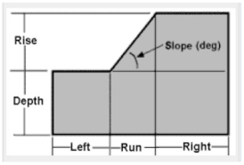
| ϕt (°) | 90 | 90 | 90 | 90 | 90 | 90 | Slope degree | 27° |
| Unit Weights | γdry (kN/m3) | 14 | 16 | 18 | 19 | 20 | 21 | ![Sustainability 14 03872 i001]() |
| γsat (kN/m3) | 19 | 20 | 21 | 19 | 20 | 21 |
| Initial Conditions | K0 (-) | 0.5 | 0.43 | 0.36 | 0.69 | 0.66 | 0.63 |
| σ0 (kPa) | 0 | 0 | 0 | 0 | 0 | 0 |
| Hydraulic Model | Kx (m/day) | 1 × 10⁻⁵ | 1 × 10⁻⁵ | 1 × 10⁻⁵ | 1 × 10⁻⁵ | 1 × 10⁻⁵ | 1 × 10⁻⁵ |
| Ky (m/day) | 1 × 10⁻⁵ | 1 × 10⁻⁵ | 1 × 10⁻⁵ | 1 × 10⁻⁵ | 1 × 10⁻⁵ | 1 × 10⁻⁵ |
| h (m) | 0.5 | 0.5 | 0.5 | 0.5 | 0.5 | 0.5 |
| Publisher’s Note: MDPI stays neutral with regard to jurisdictional claims in published maps and institutional affiliations. |
© 2022 by the authors. Licensee MDPI, Basel, Switzerland. This article is an open access article distributed under the terms and conditions of the Creative Commons Attribution (CC BY) license (https://creativecommons.org/licenses/by/4.0/).


