
Water Information Extraction Based on Multi-Model RF Algorithm and Sentinel-2 Image Data


Abstract
:1. Introduction
2. Materials and Methods
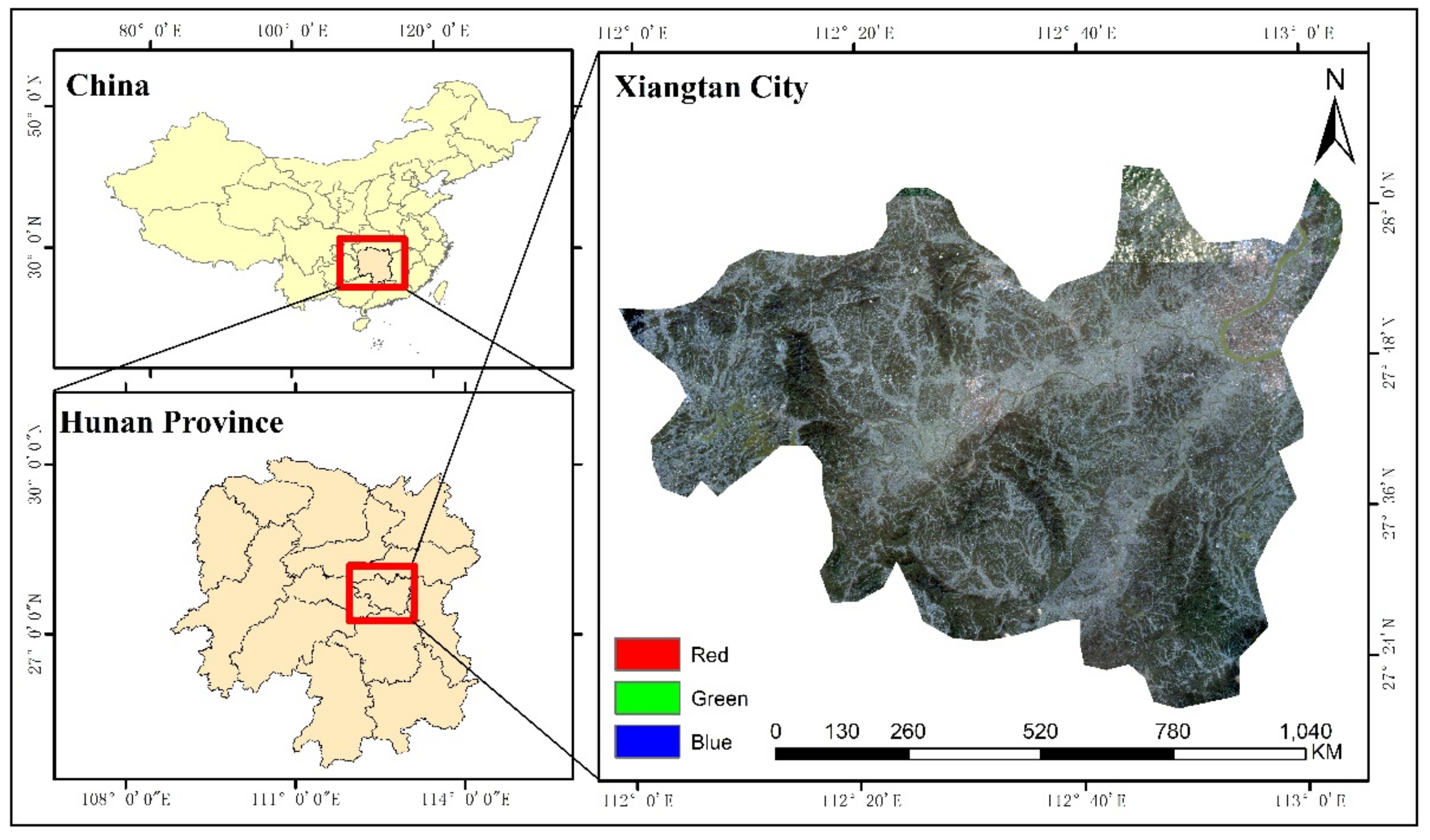
2.1. Study Area
2.2. Data Sources and Pre-Processing
Data Pre-Processing
3. Study Methods and Steps
3.1. Study Methods
3.1.1. Random Forest Algorithm
3.1.2. Accuracy Verification Algorithm
3.2. The Extraction of Characteristic Variables
3.3. Sample Selection
4. Results
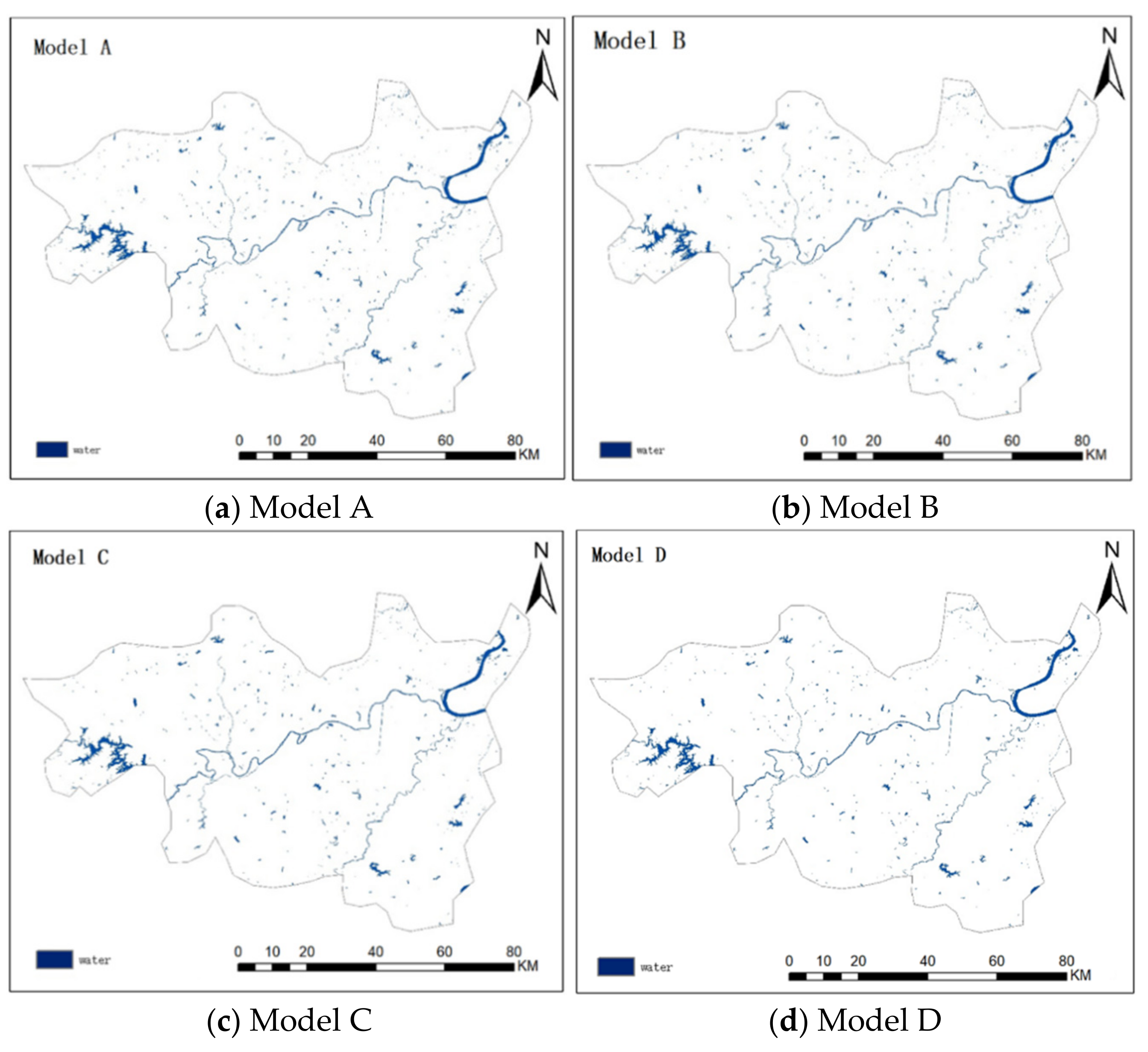
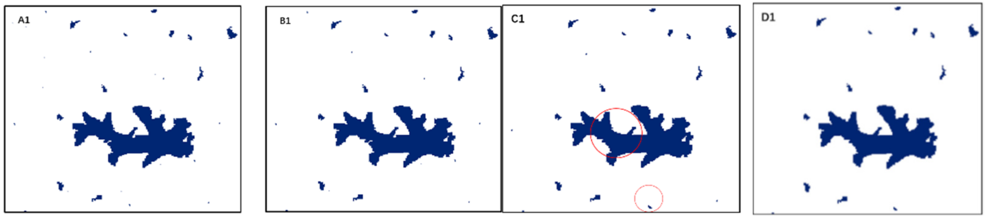
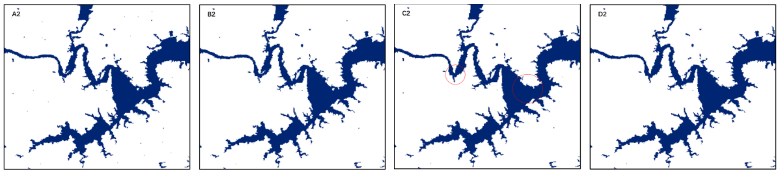
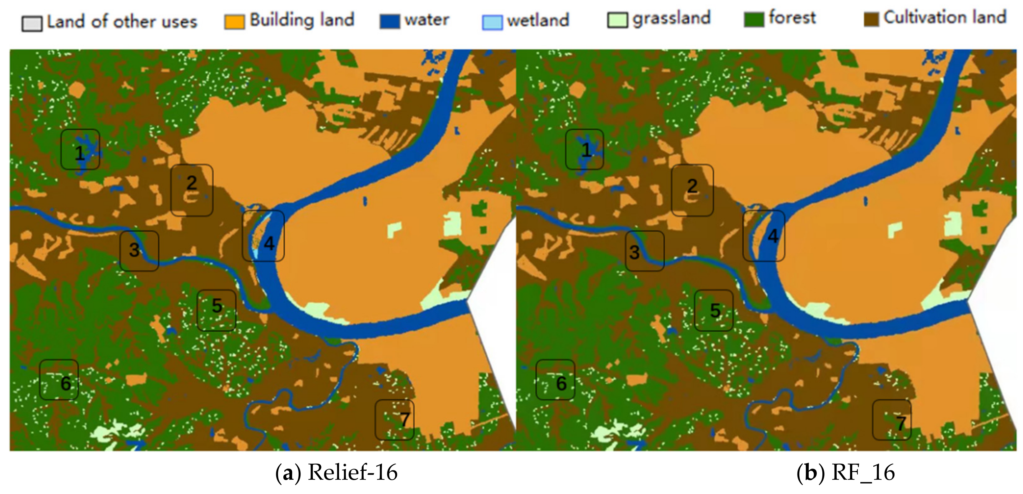
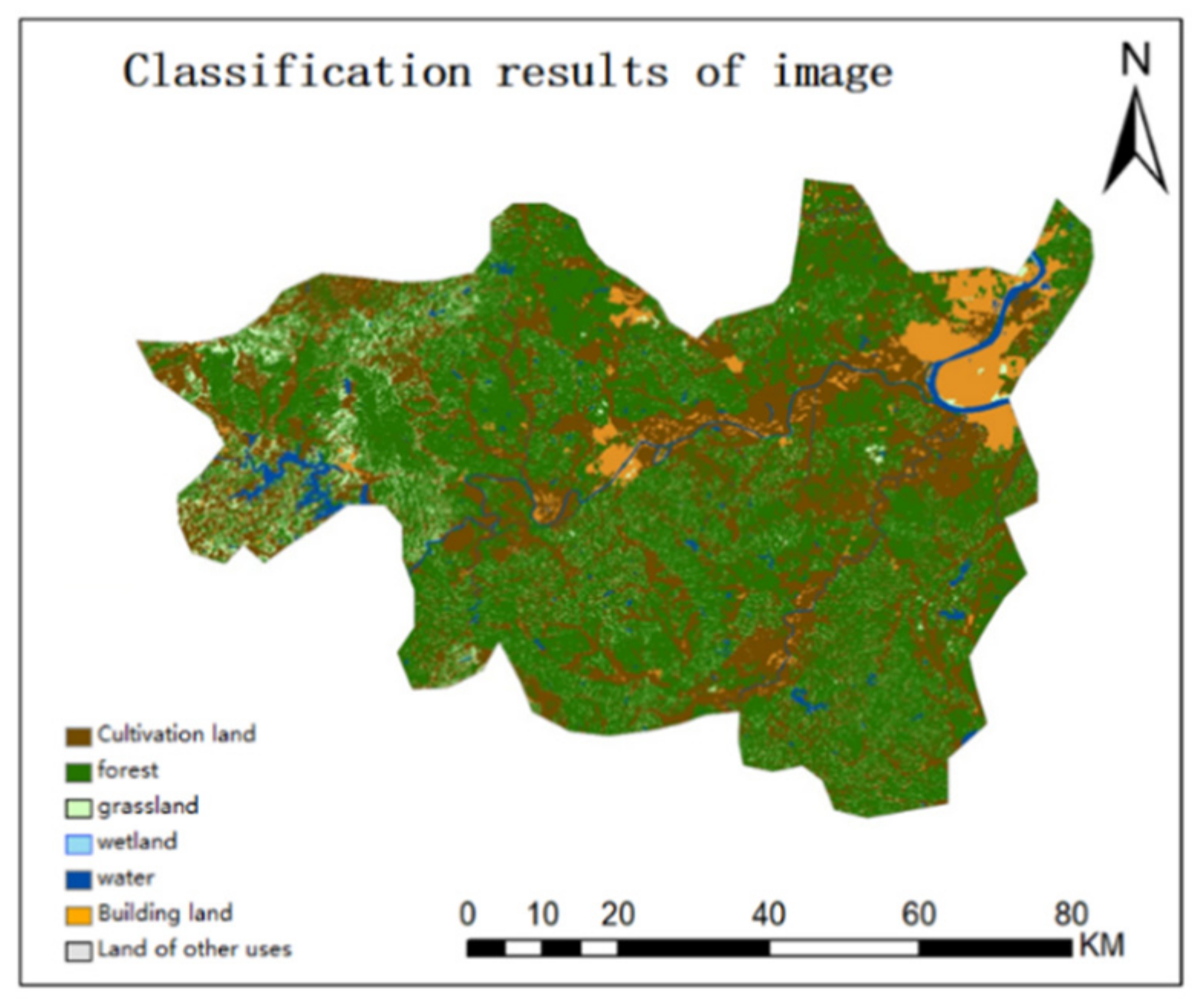
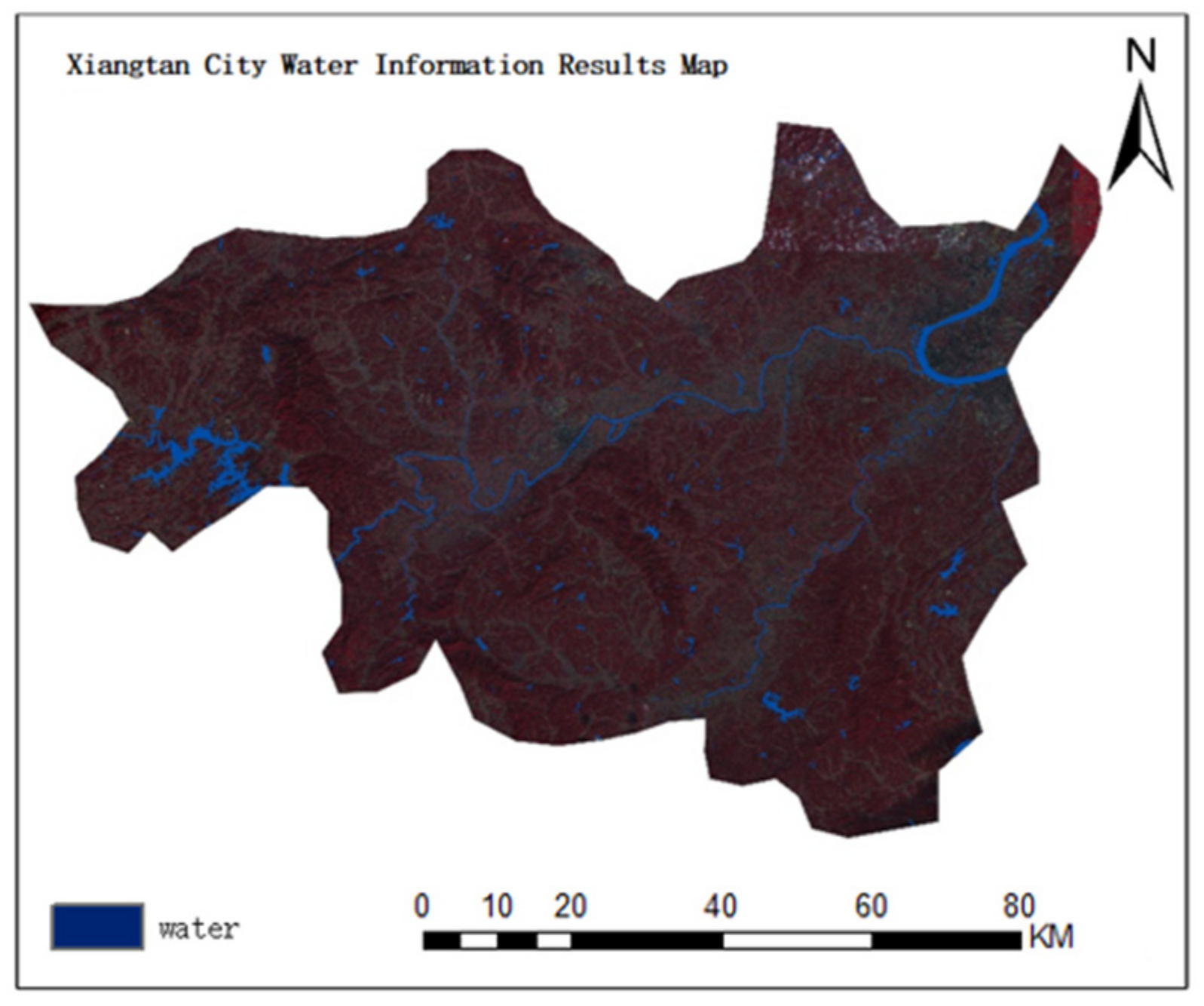
4.1. Results of Classification and Accuracy Evaluation
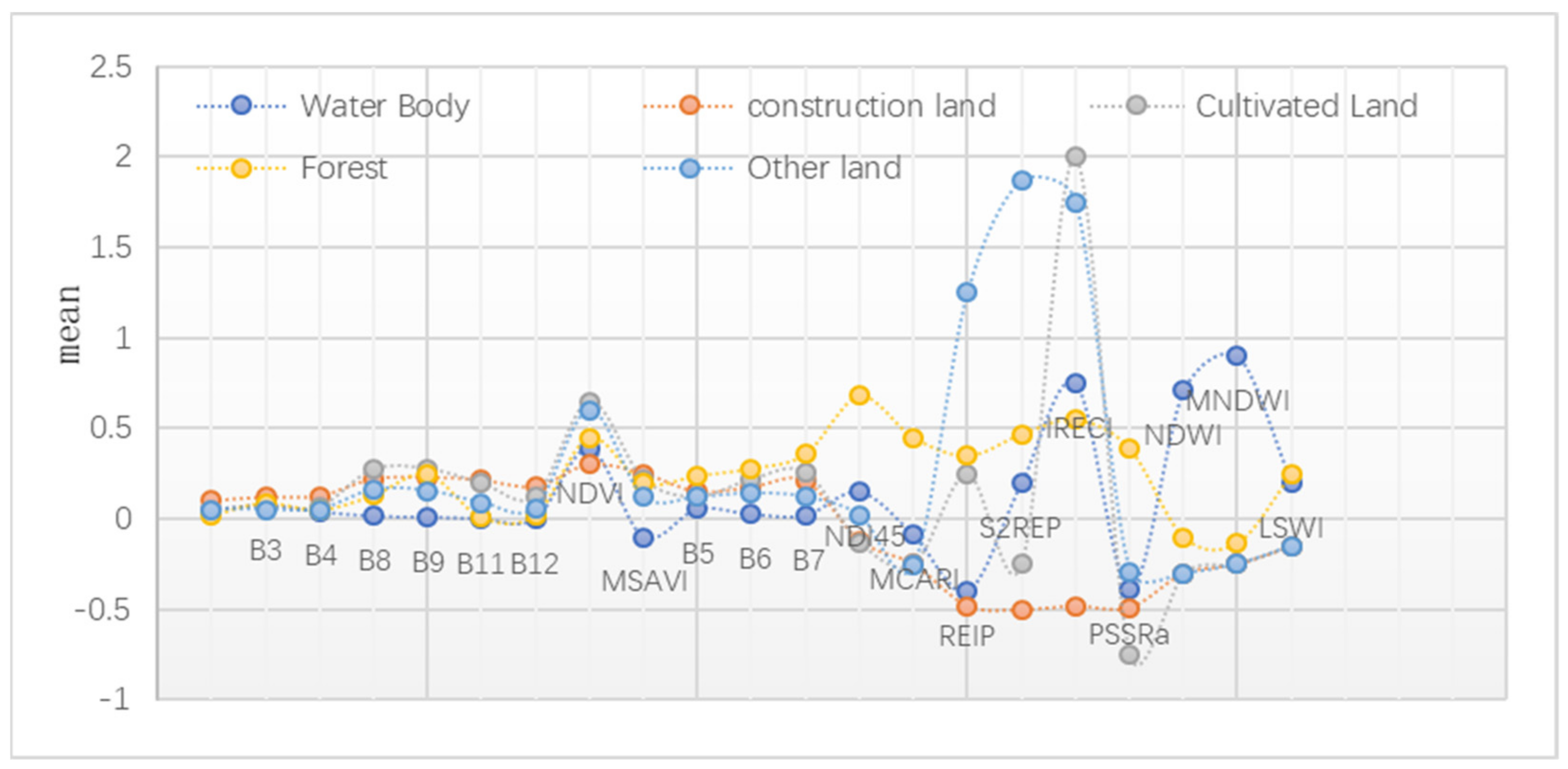
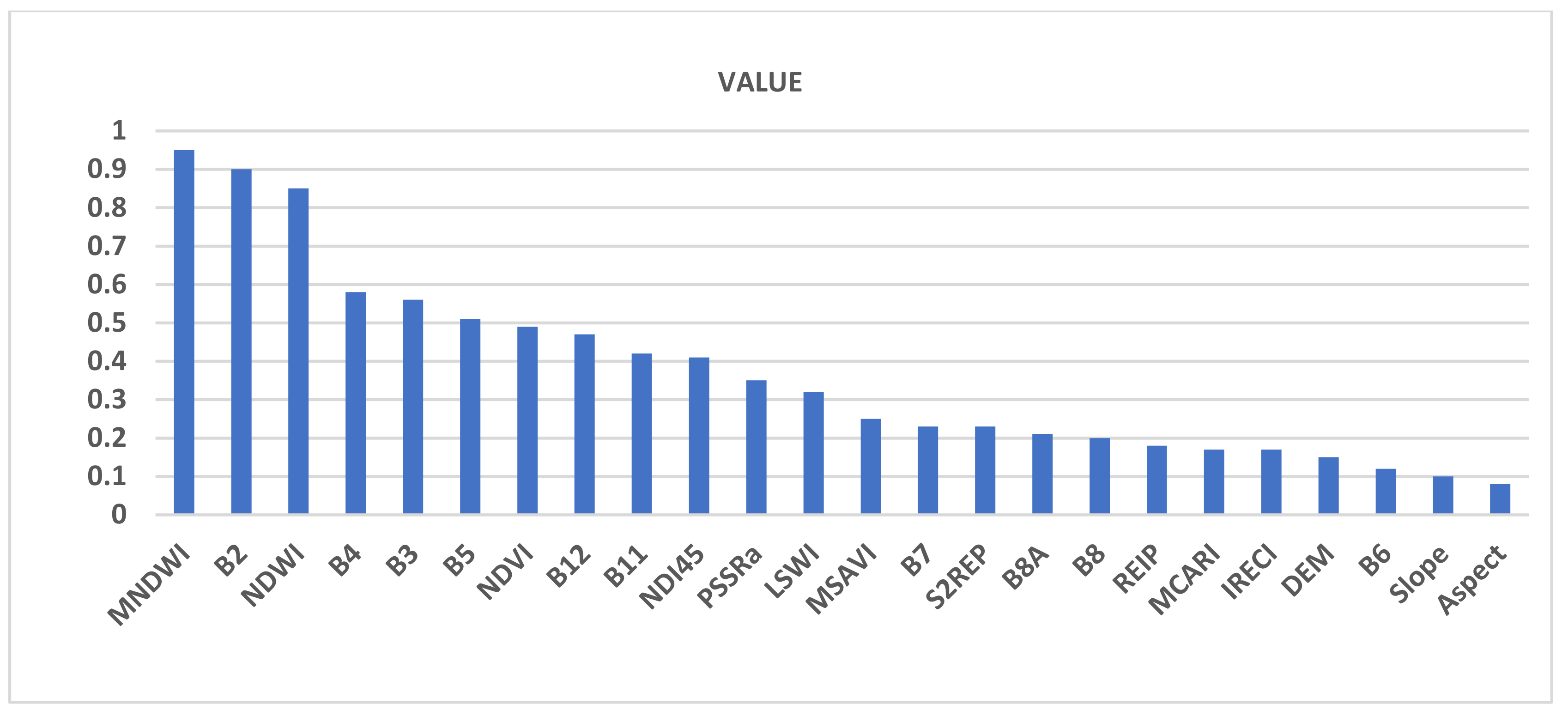
4.2. The Evaluation of Characteristic Importance
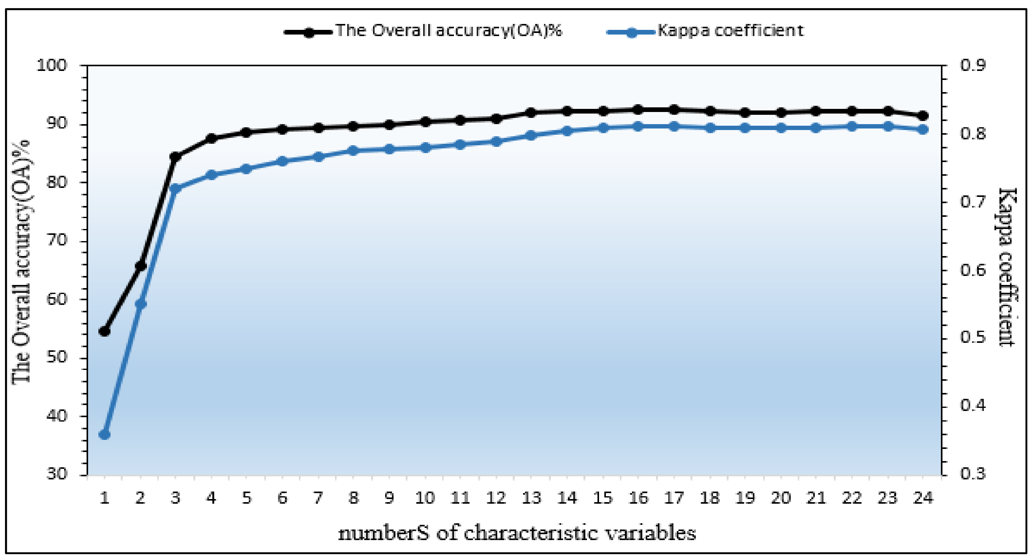
4.3. Accuracy Evaluation
5. Discussion
6. Conclusions
Author Contributions
Funding
Institutional Review Board Statement
Informed Consent Statement
Data Availability Statement
Acknowledgments
Conflicts of Interest
References
- Li, M.; Liang, H.; Guo, J.; Zhu, A. Automated Extraction of Lake Water Bodies in Complex Geographical Environments by Fusing Sentinel-1/2 Data. Water Res. 2022, 14, 30. [Google Scholar] [CrossRef]
- Du, Y.; Zhang, Y.; Ling, F.; Wang, Q.; Li, W.; Li, X. Water Bodies’ Mapping from Sentinel-2 Imagery with Modified Normalized Difference Water Index at 10 m Spatial Resolution Produced by Sharpening the SWIR Band. Remote Sens. 2016, 8, 354. [Google Scholar] [CrossRef] [Green Version]
- Loukika, K.N.; Keesara, V.R.; Sridhar, V. Analysis of Land Use and Land Cover Using Machine Learning Algorithms on Google Earth Engine for Munneru River Basin, India. Sustainability 2021, 13, 13758. [Google Scholar] [CrossRef]
- Zhu, Y.; Zhou, J.; Qiu, H.; Li, J.; Zhang, Q. Operation Rule Derivation of Hydropower Reservoirs by Support Vector Machine Based on Grey Relational Analysis. Water Res. 2021, 13, 2518. [Google Scholar] [CrossRef]
- Liu, H.; Jiang, Q.; Ma, Y.; Yang, Q.; Shi, P.; Zhang, S.; Tan, Y.; Xi, J.; Zhang, Y.; Liu, B. Object-Based Multigrained Cascade Forest Method for Wetland Classification Using Sentinel-2 and Radarsat-2 Imagery. Water Res. 2022, 14, 82. [Google Scholar] [CrossRef]
- Daho, M.; Settouti, N.; Bechar, M.; Boublenza, A.; Chikh, M.A. A new correlation-based approach for ensemble selection in random forests. Int. J. Intell. Comput. Cybern. 2021, 14, 251–268. [Google Scholar] [CrossRef]
- He, C.; Wei, J.; Song, Y.; Luo, J.-J. Seasonal Prediction of Summer Precipitation in the Middle and Lower Reaches of the Yangtze River Valley: Comparison of Machine Learning and Climate Model Predictions. Water Res. 2021, 13, 3294. [Google Scholar] [CrossRef]
- Han, H.; Choi, C.; Kim, J.; Morrison, R.R.; Jung, J.; Kim, H.S. Multiple-Depth Soil Moisture Estimates Using Artificial Neural Network and Long Short-Term Memory Models. Water Res. 2021, 13, 2584. [Google Scholar] [CrossRef]
- Chatziantoniou, A.; Psomiadis, E.; Petropoulos, G.P. Co-Orbital Sentinel 1 and 2 for LULC Mapping with Emphasis on Wetlands in a Mediterranean Setting Based on Machine Learning. Remote Sens. 2017, 9, 1259. [Google Scholar] [CrossRef] [Green Version]
- Elmahdy, S.; Ali, T.; Mohamed, M. Regional Mapping of Groundwater Potential in Ar Rub Al Khali, Arabian Peninsula Using the Classification and Regression Trees Model. Remote Sens. 2021, 13, 2300. [Google Scholar] [CrossRef]
- Weber, R. Liver-related deaths in persons infected with the human immunodeficiency virus: The D:A:D study. Arch. Internal Med. 2006, 166, 1632–1641. [Google Scholar] [CrossRef] [Green Version]
- Wafaa, M.S.; Khalid, E.; Jian, Y.; Shen, S.L. A multi-objective optimization algorithm for forecasting the compressive strength of RAC with pozzolanic materials. J. Clean. Prod. 2021, 321, 129355. [Google Scholar] [CrossRef]
- Ham, J.; Chen, Y.; Crawford, M.; Ghosh, J. Investigation of the random forest framework for classification of hyperspectral data. IEEE Trans Geosci. Remote Sens. 2005, 43, 492–501. [Google Scholar] [CrossRef] [Green Version]
- Zheng, X.; Jia, J.; Guo, S.; Chen, J.; Sun, L.; Xiong, Y.; Xu, W. Full Parameter Time Complexity (FPTC): A Method to Evaluate the Running Time of Machine Learning Classifiers for Land Use/Land Cover Classification. IEEE J. Stars 2021, 14, 2222–2235. [Google Scholar] [CrossRef]
- Tufail, R.; Ahmad, A.; Javed, M.; Sajid, R. A machine learning approach for accurate crop type mapping using combined SAR and optical time series data. Adv. Space Res. 2022, 69, 331–346. [Google Scholar] [CrossRef]
- Rodriguez-Galiano, V.F.; Ghimire, B.; Rogan, J.; Chica-Olmo, M.; Rigol-Sanchez, J.P. An assessment of the effectiveness of a random forest classifier for land-cover classification. ISPRS J. Photogramm. Remote Sens. 2011, 67, 93–104. [Google Scholar] [CrossRef]
- Topalolu, R.H.; Sertel, E.; Musaolu, N. Assessment of classification accuracies of sentinel-2 and landsat-8 data for land cover/use mapping. Int. Arch. Photogramm. Remote Sens. Spat. Inf. 2016, 41, 1055–1059. [Google Scholar] [CrossRef] [Green Version]
- Tan, Y.; Chen, H.; Xiao, W.; Meng, F.; He, T. Influence of farmland marginalization in mountainous and hilly areas on land use changes at the county level. Sci. Total Environ. 2021, 794, 149576. [Google Scholar] [CrossRef]
- Naushad, R.; Kaur, T.; Ghaderpour, E. Deep Transfer Learning for Land Use and Land Cover Classification: A Comparative Study. Sensors 2021, 21, 8083. [Google Scholar] [CrossRef]
- Forkuor, G.; Dimobe, K.; Serme, I.; Tondoh, J. Landsat-8 vs. Sentinel-2: Examining the added value of sentinel-2′s red-edge bands to land-use and land-cover mapping in Burkina Faso. GISCI Remote Sens. 2018, 55, 331–354. [Google Scholar] [CrossRef]
- Adam, E.; Mutanga, O.; Odindi, J.; Abdel-Rahman, E.M. Land-Use/Cover Classification in a Heterogeneous Coastal Landscape Using RapidEye Imagery: Evaluating the Performance of Random Forest and Support Vector Machines Classifiers. Int. J. Remote Sens. 2014, 5, 3440–3458. [Google Scholar] [CrossRef]
- Tyralis, H.; Papacharalampous, G.; Langousis, A. A Brief Review of Random Forests for Water Scientists and Practitioners and Their Recent History in Water Resources. Water Res. 2019, 11, 910. [Google Scholar] [CrossRef] [Green Version]
- Talukdar, S.; Singha, P.; Mahato, S.; Pal, S.; Liou, Y.A.; Rahman, A. Land-use land-cover classification by machine learning classifiers for satellite observations—A review. Remote Sens. 2020, 12, 1135. [Google Scholar] [CrossRef] [Green Version]
- Clark, M.L. Comparison of simulated hyperspectral HyspIRI and multispectral Landsat 8 and Sentinel-2 imagery for multi-seasonal, regional land-cover mapping. Remote Sens. Environ. 2017, 200, 311–325. [Google Scholar] [CrossRef]
- Htitiou, A.; Boudhar, A.; Lebrini, Y. The Performance of Random Forest Classification Based on Phenological Metrics Derived from Sentinel-2 and Landsat 8 to Map Crop Cover in an Irrigated Semi-arid Region. Remote Sens. Earth Syst. Sci. 2019, 2, 208–224. [Google Scholar] [CrossRef]
- Zhang, H.K.; Roy, D.P.; Yan, L.; Li, Z.; Huang, H.; Vermote, E.; Skakun, S.; Roger, J.C. Characterization of Sentinel-2A and Landsat-8 top of atmosphere, surface, and nadir BRDF adjusted reflectance and NDVI differences. Remote Sens. Environ. 2018, 215, 482–494. [Google Scholar] [CrossRef]
- Wang, J.Y.; Su, X.T.; Wang, Q.; Hao, X.Y. Land use change and its impact on ecological service value in the urban-rural interlaced zone in Xiangtan City. Hunan Agric. Sci. 2021, 6, 93–97. [Google Scholar] [CrossRef]
- Ghosh, A.; Sharma, R.; Joshi, P.K. Random forest classification of urban landscape using Landsat archive and ancillary data: Combining seasonal maps with decision level fusion. Appl. Geogr. 2014, 48, 31–41. [Google Scholar] [CrossRef]
- Ahmad, A. Performance Evaluation of Sentinel-2 and Landsat 8 OLI Data for Land Cover/Use Classification Using a Comparison between Machine Learning Algorithms. Remote Sens. 2021, 13, 1349. [Google Scholar] [CrossRef]
- DeFries, R.S.; Townshend, J.R.G. NDVI-derived land cover classifications at a global scale. Int. J. Remote Sens. 1994, 15, 3567–3586. [Google Scholar] [CrossRef]
- Zhang, Y.S.; Xie, Y.L. Vegetation Water Content Estimation Using NDVI and LSWI from MODIS Images. Sci. Geogr. Sin. 2008, 28, 72–76. [Google Scholar] [CrossRef]
- Gao, B. NDWI—A normalized difference water index for remote sensing of vegetation liquid water from space. Remote Sens. Environ. 1995, 58, 257–266. [Google Scholar] [CrossRef]
- Haboudane, D.; Miller, J.R.; Pattey, E.; Zarco-Tejada, P.J.; Strachan, I.B. Hyperspectral vegetation indices and Novel Algorithms for Predicting Green LAI of crop canopies: Modeling and Validation in the Context of Precision Agriculture. Remote Sens. Environ. 2004, 90, 337–352. [Google Scholar] [CrossRef]
- Gautam, V.K.; Gaurav, P.K.; Murugan, P. Assessment of Surface Water Dynamicsin Bangalore Using WRI, NDWI, MNDWI, Supervised Classification and K-T Transformation. Aquat. Procedia 2015, 4, 739–746. [Google Scholar] [CrossRef]
- Zhang, G.F.; Yue, C.R.; Zhang, W.Q. Inversion of aboveground biomass in Dianchi Lakeside Wetland based on Sentinel data. J. Terahertz Sci. Electron. Inf. 2020, 18, 142–149. [Google Scholar]
- Wu, C.; Niu, Z.; Tang, Q.; Huang, W. Estimating chlorophyll content from hyperspectral vegetation indices: Modeling and validation. Agric. For. Meteorol. 2008, 148, 1230–1241. [Google Scholar] [CrossRef]
- Baret, F.; Guyot, G.; Begue, A.; Maurel, P.; Podaireet, A. Complementarity of middle-infrared with visible and near-infrared reflectance for monitoring wheat canopies. Remote Sens. Environ. 1988, 26, 213–225. [Google Scholar] [CrossRef]
- Mercier, A.; Betbeder, J.; Baudry, J.; Roux, V.L.; Hubert-Moy, L. Evaluation of sentinel-1 & 2 time series for predicting wheat and rapeseed phenological stages. ISPRS J. Photogramm. 2020, 163, 231–256. [Google Scholar] [CrossRef]
- Frampton, W.J.; Dash, J.; Watmough, G.; Milton, E.J. Evaluating the capabilities of Sentinel-2 for quantitative estimation of biophysical variables in vegetation. ISPRS J. Photogramm. 2013, 82, 83–92. [Google Scholar] [CrossRef] [Green Version]
- Blackburn, G.A. Quantifying chlorophylls and caroteniods at leaf and canopy scales: An evaluation of some hyperspectral approaches. Remote Sens. Environ. 1998, 66, 273–278. [Google Scholar] [CrossRef]
- Strobl, C.; Boulesteix, A.L.; Zeileis, A.; Hothorn, T. Bias in random forest variable importance measures: Illustrations, sources and a solution. BMC Bioinform. 2007, 8, 25. [Google Scholar] [CrossRef] [Green Version]
- Sivanpillai, R.; Jacobs, K.M.; Mattilio, C.M.; Piskorski, E.V. Rapid flood inundation mapping by differencing water indices from pre-and post-flood landsat images. Front. Earth Sci. 2021, 15, 11. [Google Scholar] [CrossRef]
- Zhang, X.Y.; Li, R.; Zhen, Z.; Zhao, Y.H. Landsat-8 Remote Sensing Image Forest Vegetation Classification Based on Random Forest Model. J. Northeast. For. Univ. 2016, 44, 53–57. [Google Scholar] [CrossRef]
- Song, Y.; Si, W.; Dai, F.; Yang, G. Weighted ReliefF with threshold constraints of feature selection for imbalanced data classification. Concurr. Comput. 2020, 32, 14. [Google Scholar] [CrossRef]
- Long, Z.W.; Ji, Z.H.; Pei, Y.S. Characteristics and distribution of phosphorus in surface sediments of a shallow lake. J. Environ. Sci. 2022, 124, 50–60. [Google Scholar] [CrossRef]
- Immitzer, M.; Vuolo, F.; Atzberger, C. First Experience with Sentinel-2 Data for Crop and Tree Species Classifications in Central Europe. Remote Sens. 2016, 8, 166. [Google Scholar] [CrossRef]


| Sentinel-2 Bands | Center Wavelength (nm) | Spectral Width (nm) | Spatial Resolution (m) |
|---|---|---|---|
| Band 1-Coastal aerosol | 443 | 20 | 60 |
| Band 2-Blue | 490 | 65 | 10 |
| Band 3-Green | 560 | 35 | 10 |
| Band 4-Red | 665 | 30 | 10 |
| Band 5-Vegetation Red-Edge 1 | 705 | 15 | 20 |
| Band 6-Vegetation Red-Edge 2 | 740 | 15 | 20 |
| Band 7-Vegetation Red-Edge 3 | 783 | 20 | 20 |
| Band 8-NIR | 842 | 115 | 10 |
| Band 8a-Vegetation Red-Edge 4 | 865 | 20 | 20 |
| Band 11-SWIR1 | 1610 | 90 | 20 |
| Band 12-SWIR2 | 2190 | 180 | 20 |
| Abbreviations | Full Names | Calculation Formulas | Types | Citations |
|---|---|---|---|---|
| NDVI | Normalized Difference Vegetation Indices | (B8 − B4)/(B8 + B4) | Traditional Spectral Indices Characteristics | [30] |
| LSWI | Land Surface Water Indices | (B8 − B11)/(B8 + B11) | Traditional Spectral Indices Characteristics | [31] |
| NDWI | Normalized Difference Water Indices | (B8 − B4)/(B8 + B4) | Traditional Spectral Indices Characteristics | [32] |
| MSAVI | Modified Soil Adjusted Vegetation Indices | 0.5 × (2 × (B8+1) − sqrt((2 × B8 + 1)2 − 8 × (B8 − B4))) | Traditional Spectral Indices Characteristics | [33] |
| MNDWI | Modified Normalized Difference Water Indices | (B3 − B11)/(B3 + B11) | Traditional Spectral Indices Characteristics | [34] |
| NDI45 | Normalized Difference Indices | (B5 − B4)/(B5 + B4) | Red-Edge Spectral Indices Characteristics | [35] |
| MCARI | Modified Chlorophyll Absorption Ratio Indices | [(B5 − B4) − 0.2 × (B5 − B3)] × (B5 − B4) | Red-Edge Spectral Indices Characteristics | [36] |
| REIP | Red-Edge Inflection Point Indices | 700 + 40 × ((B4 + B7)/2 − B5)/(B6 − B5) | Red-Edge Spectral Indices Characteristics | [37] |
| S2REP | The Sentinel-2 Red-Edge Position Indices | 705 + 35 × ((B4 + B7)/2 − B5)/(B6 − B5) | Red-Edge Spectral Indices Characteristics | [38] |
| IRECI | Inverted Red-Edge Chlorophyll Indices | (B7 − B4)/(B5/B6) | Red-Edge Spectral Indices Characteristics | [39] |
| PSSRa | Pigment Specific Simple Ratio(chlorophyll) Indices. | B7/B4 | Red-Edge Spectral Indices Characteristics | [40] |
| Characteristic Class | Training Samples | Validation Samples | Total Number of Samples |
|---|---|---|---|
| Water | 927 | 463 | 1390 |
| Cultivated land | 1233 | 616 | 1849 |
| Forest land | 1996 | 991 | 2987 |
| Grass land | 146 | 73 | 219 |
| Wetland | 104 | 52 | 156 |
| Construction land | 251 | 125 | 376 |
| Other land | 166 | 83 | 249 |
| Types | Model A | Model B | Model C | Model D | ||||
|---|---|---|---|---|---|---|---|---|
| Producer’s Accuracy | User’s Accuracy | Producer’s Accuracy | User’s Accuracy | Producer’s Accuracy | User’s Accuracy | Producer’s Accuracy | User’s Accuracy | |
| (PA) | (UA) | (PA) | (UA) | (PA) | (UA) | (PA) | (UA) | |
| Water | 80.63 | 83.22 | 82.16 | 86.22 | 91.39 | 94.12 | 92.16 | 95.22 |
| Cultivation land | 85.43 | 79.26 | 88.52 | 81.53 | 89.21 | 82.46 | 91.25 | 84.53 |
| Forest | 90.45 | 92.76 | 92.87 | 93.98 | 93.07 | 94.19 | 93.98 | 95.06 |
| Grassland | 82.36 | 76.52 | 84.51 | 79.84 | 87.12 | 81.65 | 90.12 | 83.54 |
| Wetland | 80.15 | 73.28 | 85.62 | 80.17 | 87.45 | 81.56 | 90.22 | 93.14 |
| Building land | 82.03 | 73.49 | 80.41 | 71.29 | 83.46 | 79.02 | 86.52 | 81.39 |
| Others | 85.87 | 81.37 | 88.41 | 81.61 | 91.67 | 84.62 | 94.67 | 88.62 |
| The overall accuracy (OA)% | 81.24 | 86.39 | 89.71 | 92.37 | ||||
| Kappa coefficient | 0.8016 | 0.8092 | 0.8114 | 0.8116 | ||||
| Types | RF_16 | Relief-16 | Model D | |||
|---|---|---|---|---|---|---|
| Producer’s Accuracy | User’s Accuracy | Producer’s Accuracy | User’s Accuracy | Producer’s Accuracy | User’s Accuracy | |
| (PA) | (UA) | (PA) | (UA) | (PA) | (UA) | |
| Water | 94.16 | 96.22 | 92.39 | 95.42 | 92.16 | 95.22 |
| Cultivation land | 90.12 | 88.53 | 92.21 | 85.46 | 91.25 | 84.53 |
| Forest | 93.87 | 94.98 | 93.17 | 94.19 | 93.98 | 95.06 |
| Grassland | 91.51 | 88.34 | 91.12 | 84.65 | 90.12 | 83.54 |
| Wetland | 93.62 | 90.17 | 92.45 | 91.56 | 90.22 | 93.14 |
| Building land | 91.41 | 89.29 | 89.56 | 85.02 | 86.52 | 81.39 |
| Others | 94.81 | 92.61 | 91.67 | 89.62 | 94.67 | 88.62 |
| The overall accuracy (OA)% | 93.16 | 93.04 | 92.37 | |||
| Kappa coefficient | 0.8224 | 0.8176 | 0.8116 | |||
| Methods | Kappa Coefficient | Missed Extraction Rate/% | False Extraction Rate /% | The Overall Accuracy (OA)% |
|---|---|---|---|---|
| NDVI | 0.8046 | 2.86 | 13.72 | 89.22 |
| NDWI | 0.8112 | 1.94 | 11.24 | 90.12 |
| MNDWI | 0.8206 | 1.89 | 10.56 | 92.57 |
| RF_16 | 0.8224 | 0.48 | 7.22 | 93.16 |
| Methods | Extraction Effect | First Area | Second Area | Third Area |
|---|---|---|---|---|
| NDVI |  |  |  |  |
| NDWI |  |  |  |  |
| MNDWI |  |  | 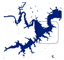 | 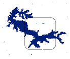 |
| RF_16 | 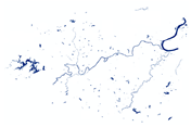 | 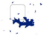 |  |  |
Publisher’s Note: MDPI stays neutral with regard to jurisdictional claims in published maps and institutional affiliations. |
© 2022 by the authors. Licensee MDPI, Basel, Switzerland. This article is an open access article distributed under the terms and conditions of the Creative Commons Attribution (CC BY) license (https://creativecommons.org/licenses/by/4.0/).
Share and Cite
Jiang, Z.; Wen, Y.; Zhang, G.; Wu, X. Water Information Extraction Based on Multi-Model RF Algorithm and Sentinel-2 Image Data. Sustainability 2022, 14, 3797. https://doi.org/10.3390/su14073797
Jiang Z, Wen Y, Zhang G, Wu X. Water Information Extraction Based on Multi-Model RF Algorithm and Sentinel-2 Image Data. Sustainability. 2022; 14(7):3797. https://doi.org/10.3390/su14073797
Chicago/Turabian StyleJiang, Zhiqi, Yijun Wen, Gui Zhang, and Xin Wu. 2022. "Water Information Extraction Based on Multi-Model RF Algorithm and Sentinel-2 Image Data" Sustainability 14, no. 7: 3797. https://doi.org/10.3390/su14073797
APA StyleJiang, Z., Wen, Y., Zhang, G., & Wu, X. (2022). Water Information Extraction Based on Multi-Model RF Algorithm and Sentinel-2 Image Data. Sustainability, 14(7), 3797. https://doi.org/10.3390/su14073797