
Investigation of Small-Scale Photovoltaic Systems for Optimum Performance under Partial Shading Conditions


Abstract
1. Introduction
1.1. Motivation
1.2. Literature Review
1.3. Novelty of Work
- It provides a comprehensive investigation of the performance of small PV systems (consisting of 10 modules or fewer) rather than for large systems as in most previous studies.
- PV systems are tested under all possible shading patterns as a result of a single shading level (300 W/m2) for common wiring configurations rather than for a set number of patterns as in previous studies.
- To be able to cover all possible PS patterns, a new reduction methodology is proposed to eliminate the equivalent patterns. Consequently, the number of studied patterns is limited to a feasible value as low as 100 cases.
- The study affords a few recommendations for the proper choice of the PV system configuration, seeking optimum performance under PS conditions.
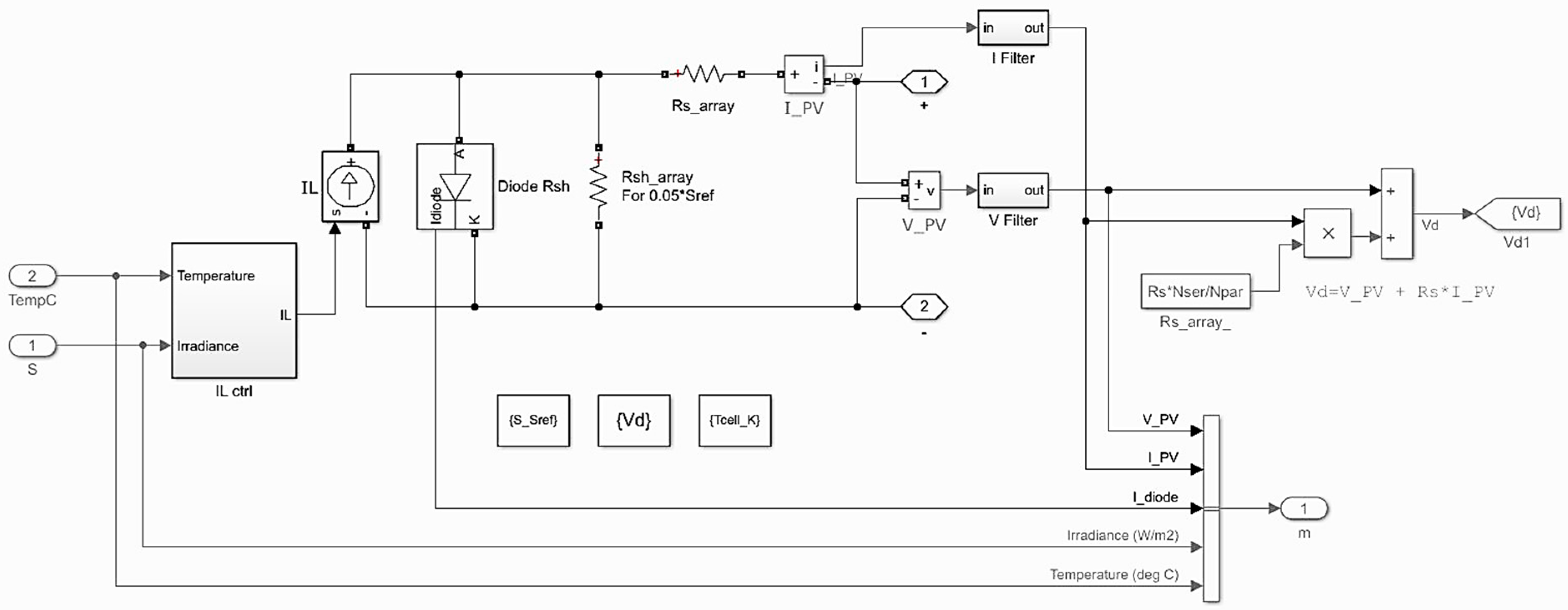
2. Mathematical Modeling
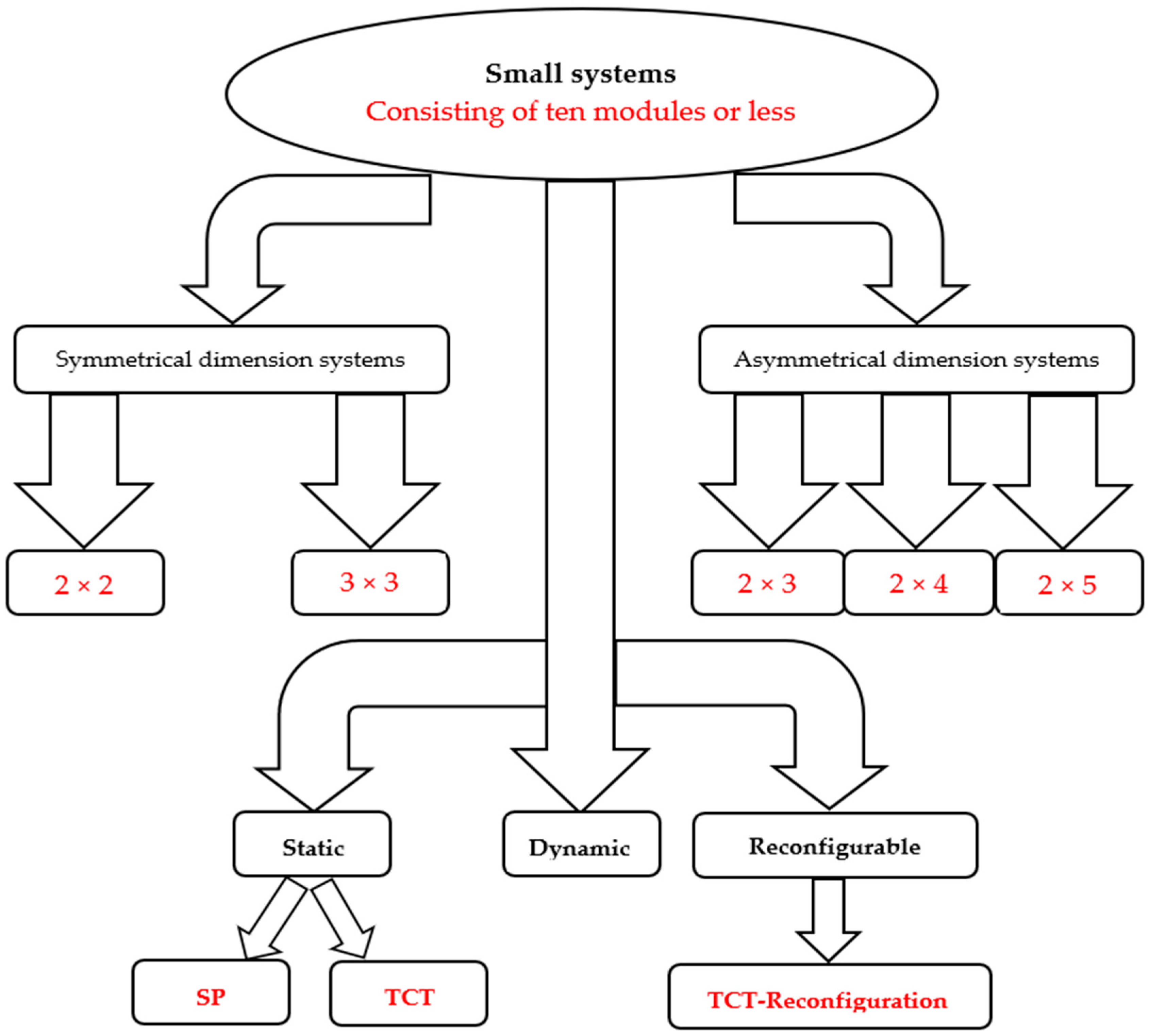
3. System Description
- i.
- Symmetrical dimension systems: symmetrical systems that consist of 10 modules or fewer with equal numbers of rows and columns are mainly configured in two systems (2 × 2) and (3 × 3).
- ii.
- Asymmetrical dimension systems: asymmetrical systems are those in which the number of rows is not equal to the number of columns. Asymmetrical systems that consist of 10 modules or fewer are mainly configured in three systems (2 × 3), (2 × 4), and (2 × 5).
4. Shading Patterns Description
5. Performance Parameters
6. Simulation Results and Discussion
6.1. Symmetrical Dimension Systems
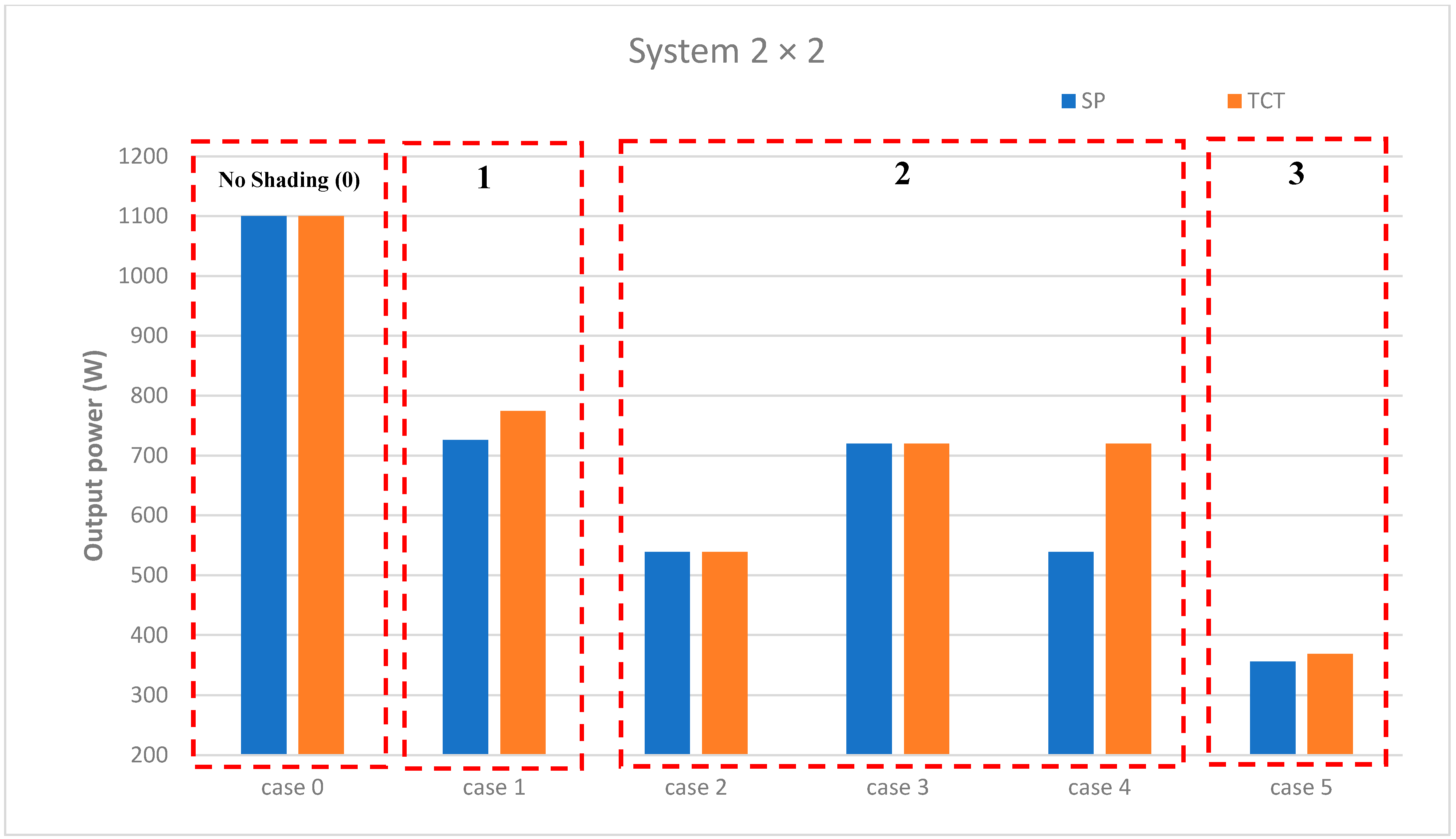
6.1.1. System 2 × 2
6.1.2. System 3 × 3
6.2. Asymmetrical Dimension Systems
6.2.1. System 2 × 3
6.2.2. System 2 × 4
6.2.3. System 2 × 5
7. Conclusions
Author Contributions
Funding
Institutional Review Board Statement
Informed Consent Statement
Data Availability Statement
Conflicts of Interest
Appendix A

| Case Number. | Number of Shaded Modules | Partial Shading Pattern | Series-Parallel | Total-Cross-Tied | KT% | KRT% | |||||||||||||||||
|---|---|---|---|---|---|---|---|---|---|---|---|---|---|---|---|---|---|---|---|---|---|---|---|
| VOC | ISC | VGMPP | IGMPP | PGMPP | PL % | Efficiency % | Number of Local MPPs | VOC | ISC | VGMPP | IGMPP | PGMPP | PL % | Efficiency % | Number of Local MPPs | ||||||||
| 0 | 0 | 0 | 89.4 | 16.7 | 70.2 | 15.7 | 1100 | 0.00 | 14.17 | 1 | 89.4 | 16.7 | 70.2 | 15.7 | 1100 | 0.00 | 14.17 | 1 | 0.00 | 0.00 | |||
| 0 | |||||||||||||||||||||||
| 0 | 0 | ||||||||||||||||||||||
| 1 | 1 | 1 | 88.5 | 16.7 | 71.3 | 10.2 | 726.2 | 33.98 | 9.36 | 2 | 88.5 | 16.7 | 73.9 | 10.5 | 774.6 | 29.58 | 9.98 | 2 | 6.25 | 0.00 | |||
| 0 | |||||||||||||||||||||||
| 1 | 0 | ||||||||||||||||||||||
| 2 | 2 | 2 | 87.3 | 16.7 | 34.4 | 15.7 | 539.1 | 50.99 | 6.95 | 2 | 87.3 | 16.7 | 34.4 | 15.7 | 539.1 | 50.99 | 6.95 | 2 | 0.00 | 25.09 | |||
| 0 | |||||||||||||||||||||||
| 1 | 1 | ||||||||||||||||||||||
| 3 | 1 | 87.7 | 10.8 | 70.6 | 10.2 | 719.7 | 34.57 | 9.27 | 1 | 87.7 | 10.8 | 70.6 | 10.2 | 719.7 | 34.57 | 9.27 | 1 | 0.00 | 0.00 | ||||
| 1 | |||||||||||||||||||||||
| 2 | 0 | ||||||||||||||||||||||
| 4 | 1 | 87.3 | 16.7 | 34.4 | 15.7 | 539.1 | 50.99 | 6.95 | 2 | 87.7 | 10.8 | 70.6 | 10.2 | 719.7 | 34.57 | 9.27 | 1 | 25.09 | 0.00 | ||||
| 1 | |||||||||||||||||||||||
| 1 | 1 | ||||||||||||||||||||||
| 5 | 3 | 2 | 86.3 | 10.8 | 35 | 10.2 | 356.1 | 67.63 | 4.59 | 2 | 86.5 | 10.8 | 76 | 4.85 | 369 | 66.45 | 4.75 | 2 | 3.50 | 0.00 | |||
| 1 | |||||||||||||||||||||||
| 2 | 1 | ||||||||||||||||||||||

| Case Number. | Number of Shaded Modules | Partial Shading Pattern | Series-Parallel | Total-Cross-Tied | KT% | KRT% | |||||||||||||||||
|---|---|---|---|---|---|---|---|---|---|---|---|---|---|---|---|---|---|---|---|---|---|---|---|
| VOC | ISC | VGMPP | IGMPP | PGMPP | PL % | Efficiency % | Number of Local MPPs | VOC | ISC | VGMPP | IGMPP | PGMPP | PL % | Efficiency % | Number of Local MPPs | ||||||||
| 0 | 0 | 0 | 134.1 | 25 | 105.4 | 23.5 | 2476 | 0.00 | 14.18 | 1 | 134.1 | 25 | 105.4 | 23.5 | 2476 | 0.00 | 14.18 | 1 | 0.00 | 0.00 | |||
| 0 | |||||||||||||||||||||||
| 0 | |||||||||||||||||||||||
| 0 | 0 | 0 | |||||||||||||||||||||
| 1 | 1 | 1 | 133.4 | 25 | 106.3 | 18 | 1914 | 22.70 | 10.96 | 2 | 133.5 | 25 | 110.7 | 18.7 | 2067 | 16.52 | 11.84 | 2 | 7.40 | 0.00 | |||
| 0 | |||||||||||||||||||||||
| 0 | |||||||||||||||||||||||
| 1 | 0 | 0 | |||||||||||||||||||||
| 2 | 2 | 2 | 132.8 | 25 | 71.4 | 23.5 | 1674 | 32.39 | 9.59 | 2 | 132.9 | 25 | 69.6 | 23.5 | 1634 | 34.01 | 9.36 | 2 | −2.45 | 17.39 | |||
| 0 | |||||||||||||||||||||||
| 0 | |||||||||||||||||||||||
| 1 | 1 | 0 | |||||||||||||||||||||
| 3 | 1 | 132.9 | 25 | 106.1 | 18 | 1912 | 22.78 | 10.95 | 2 | 133 | 25 | 107.9 | 18.3 | 1978 | 20.11 | 11.33 | 2 | 3.34 | 0.00 | ||||
| 1 | |||||||||||||||||||||||
| 0 | |||||||||||||||||||||||
| 2 | 0 | 0 | |||||||||||||||||||||
| 4 | 1 | 132.8 | 25 | 71.4 | 23.5 | 1674 | 32.39 | 9.59 | 2 | 133 | 25 | 107.9 | 18.3 | 1978 | 20.11 | 11.33 | 2 | 15.37 | 0.00 | ||||
| 1 | |||||||||||||||||||||||
| 0 | |||||||||||||||||||||||
| 1 | 1 | 0 | |||||||||||||||||||||
| 5 | 3 | 3 | 132 | 25 | 96.6 | 23.5 | 1634 | 34.01 | 9.36 | 2 | 132 | 25 | 96.6 | 23.5 | 1634 | 34.01 | 9.36 | 2 | 0.00 | 14.23 | |||
| 0 | |||||||||||||||||||||||
| 0 | |||||||||||||||||||||||
| 1 | 1 | 1 | |||||||||||||||||||||
| 6 | 2 | 132.1 | 25 | 108.2 | 12.5 | 1355 | 45.27 | 7.76 | 3 | 132.3 | 25 | 113.7 | 13 | 1481 | 40.19 | 8.48 | 3 | 8.51 | 22.26 | ||||
| 1 | |||||||||||||||||||||||
| 0 | |||||||||||||||||||||||
| 2 | 1 | 0 | |||||||||||||||||||||
| 7 | 2 | 132 | 25 | 96.6 | 23.5 | 1634 | 34.01 | 9.36 | 2 | 132.3 | 25 | 113.7 | 13 | 1481 | 40.19 | 8.48 | 3 | −10.33 | 22.26 | ||||
| 1 | |||||||||||||||||||||||
| 0 | |||||||||||||||||||||||
| 1 | 1 | 1 | |||||||||||||||||||||
| 8 | 1 | 132.4 | 19.2 | 105.6 | 18 | 1905 | 23.06 | 10.91 | 1 | 132.4 | 19.2 | 105.6 | 18 | 1905 | 23.06 | 10.91 | 1 | 0.00 | 0.00 | ||||
| 1 | |||||||||||||||||||||||
| 1 | |||||||||||||||||||||||
| 3 | 0 | 0 | |||||||||||||||||||||
| 9 | 1 | 132.1 | 25 | 108.2 | 12.5 | 1355 | 45.27 | 7.76 | 3 | 132.4 | 19.2 | 105.6 | 18 | 1905 | 23.06 | 10.91 | 1 | 28.87 | 0.00 | ||||
| 1 | |||||||||||||||||||||||
| 1 | |||||||||||||||||||||||
| 2 | 1 | 0 | |||||||||||||||||||||
| 10 | 1 | 132 | 25 | 96.6 | 23.5 | 1634 | 34.01 | 9.36 | 2 | 132.4 | 19.2 | 105.6 | 18 | 1905 | 23.06 | 10.91 | 1 | 14.23 | 0.00 | ||||
| 1 | |||||||||||||||||||||||
| 1 | |||||||||||||||||||||||
| 1 | 1 | 1 | |||||||||||||||||||||
| 11 | 4 | 3 | 131.3 | 25 | 70.1 | 18 | 1263 | 48.99 | 7.23 | 3 | 131.5 | 25 | 72.1 | 18.5 | 1334 | 46.12 | 7.64 | 3 | 5.32 | 8.76 | |||
| 1 | |||||||||||||||||||||||
| 0 | |||||||||||||||||||||||
| 2 | 1 | 1 | |||||||||||||||||||||
| 12 | 2 | 131.6 | 19.2 | 107.2 | 12.54 | 1345 | 45.68 | 7.70 | 2 | 131.8 | 19.2 | 112.3 | 13 | 1462 | 40.95 | 8.37 | 2 | 8.00 | 0.00 | ||||
| 1 | |||||||||||||||||||||||
| 1 | |||||||||||||||||||||||
| 3 | 1 | 0 | |||||||||||||||||||||
| 13 | 2 | 131.6 | 25 | 107.9 | 12.5 | 1353 | 45.36 | 7.75 | 2 | 131.7 | 25 | 110.2 | 12.8 | 1410 | 43.05 | 8.07 | 2 | 4.04 | 3.56 | ||||
| 2 | |||||||||||||||||||||||
| 0 | |||||||||||||||||||||||
| 2 | 2 | 0 | |||||||||||||||||||||
| 14 | 2 | 131.3 | 25 | 70.1 | 18 | 1263 | 48.99 | 7.23 | 3 | 131.7 | 25 | 110.2 | 12.8 | 1410 | 43.05 | 8.07 | 2 | 10.43 | 3.56 | ||||
| 2 | |||||||||||||||||||||||
| 0 | |||||||||||||||||||||||
| 1 | 2 | 1 | |||||||||||||||||||||
| 15 | 2 | 131.3 | 25 | 70.1 | 18 | 1263 | 48.99 | 7.23 | 3 | 131.8 | 19.2 | 112.3 | 13 | 1462 | 40.95 | 8.37 | 2 | 13.61 | 0.00 | ||||
| 1 | |||||||||||||||||||||||
| 1 | |||||||||||||||||||||||
| 1 | 1 | 2 | |||||||||||||||||||||
| 16 | 1 | 131.6 | 25 | 107.9 | 12.5 | 1353 | 45.36 | 7.75 | 2 | 131.8 | 19.2 | 112.3 | 13 | 1462 | 40.95 | 8.37 | 2 | 7.46 | 0.00 | ||||
| 2 | |||||||||||||||||||||||
| 1 | |||||||||||||||||||||||
| 2 | 2 | 0 | |||||||||||||||||||||
| 17 | 5 | 3 | 130.7 | 25 | 71.6 | 12.5 | 897 | 63.77 | 5.14 | 3 | 130.8 | 25 | 74.3 | 12.9 | 959.4 | 61.25 | 5.49 | 3 | 6.50 | 31.08 | |||
| 2 | |||||||||||||||||||||||
| 0 | |||||||||||||||||||||||
| 2 | 2 | 1 | |||||||||||||||||||||
| 18 | 2 | 131 | 19.2 | 107 | 12.6 | 1343 | 45.76 | 7.69 | 2 | 131.1 | 19.2 | 108.9 | 12.8 | 1392 | 43.78 | 7.97 | 2 | 3.52 | 0.00 | ||||
| 2 | |||||||||||||||||||||||
| 1 | |||||||||||||||||||||||
| 3 | 2 | 0 | |||||||||||||||||||||
| 19 | 2 | 130.7 | 25 | 71.6 | 12.5 | 897 | 63.77 | 5.14 | 3 | 131.1 | 19.2 | 108.9 | 12.8 | 1392 | 43.78 | 7.97 | 2 | 35.56 | 0.00 | ||||
| 2 | |||||||||||||||||||||||
| 1 | |||||||||||||||||||||||
| 2 | 1 | 2 | |||||||||||||||||||||
| 20 | 3 | 130.7 | 25 | 71.6 | 12.5 | 897 | 63.77 | 5.14 | 3 | 130.9 | 19.2 | 69.8 | 18 | 1257 | 49.23 | 7.20 | 2 | 28.64 | 9.70 | ||||
| 1 | |||||||||||||||||||||||
| 1 | |||||||||||||||||||||||
| 2 | 1 | 2 | |||||||||||||||||||||
| 21 | 2 | 130.8 | 19.2 | 70.1 | 18 | 1263 | 48.99 | 7.23 | 2 | 131.1 | 19.2 | 108.9 | 12.8 | 1392 | 43.78 | 7.97 | 2 | 9.27 | 0.00 | ||||
| 1 | |||||||||||||||||||||||
| 2 | |||||||||||||||||||||||
| 3 | 1 | 1 | |||||||||||||||||||||
| 22 | 3 | 130.8 | 19.2 | 70.1 | 18 | 1263 | 48.99 | 7.23 | 2 | 130.9 | 19.2 | 69.8 | 18 | 1257 | 49.23 | 7.20 | 2 | −0.48 | 9.70 | ||||
| 1 | |||||||||||||||||||||||
| 1 | |||||||||||||||||||||||
| 3 | 1 | 1 | |||||||||||||||||||||
| 23 | 6 | 3 | 129.9 | 25 | 113.2 | 7.2 | 817.3 | 66.99 | 4.68 | 2 | 129.9 | 25 | 113.2 | 7.2 | 817.3 | 66.99 | 4.68 | 2 | 0.00 | 38.73 | |||
| 3 | |||||||||||||||||||||||
| 0 | |||||||||||||||||||||||
| 2 | 2 | 2 | |||||||||||||||||||||
| 24 | 2 | 130.5 | 13.3 | 106.3 | 12.6 | 1334 | 46.12 | 7.64 | 1 | 130.5 | 13.3 | 106.3 | 12.6 | 1334 | 46.12 | 7.64 | 1 | 0.00 | 0.00 | ||||
| 2 | |||||||||||||||||||||||
| 2 | |||||||||||||||||||||||
| 3 | 3 | 0 | |||||||||||||||||||||
| 25 | 3 | 130 | 19.1 | 71.7 | 12.5 | 896.7 | 63.78 | 5.13 | 3 | 130.3 | 19.2 | 73 | 12.9 | 941.2 | 61.99 | 5.39 | 3 | 4.73 | 29.45 | ||||
| 2 | |||||||||||||||||||||||
| 1 | |||||||||||||||||||||||
| 3 | 2 | 1 | |||||||||||||||||||||
| 26 | 2 | 129.9 | 25 | 113.2 | 7.2 | 817.3 | 66.99 | 4.68 | 2 | 130.5 | 13.3 | 106.3 | 12.6 | 1334 | 46.12 | 7.64 | 1 | 38.73 | 0.00 | ||||
| 2 | |||||||||||||||||||||||
| 2 | |||||||||||||||||||||||
| 2 | 2 | 2 | |||||||||||||||||||||
| 27 | 3 | 129.9 | 25 | 113.2 | 7.2 | 817.3 | 66.99 | 4.68 | 2 | 130.3 | 19.2 | 73 | 12.9 | 941.2 | 61.99 | 5.39 | 3 | 13.16 | 29.45 | ||||
| 2 | |||||||||||||||||||||||
| 1 | |||||||||||||||||||||||
| 2 | 2 | 2 | |||||||||||||||||||||
| 28 | 2 | 130 | 19.1 | 71.7 | 12.5 | 896.7 | 63.78 | 5.13 | 3 | 130.5 | 13.3 | 106.3 | 12.6 | 1334 | 46.12 | 7.64 | 1 | 32.78 | 0.00 | ||||
| 2 | |||||||||||||||||||||||
| 2 | |||||||||||||||||||||||
| 3 | 2 | 1 | |||||||||||||||||||||
| 29 | 7 | 3 | 129.3 | 19.2 | 111.1 | 7.2 | 759.2 | 69.34 | 4.35 | 2 | 129.3 | 19.2 | 112.3 | 7.2 | 811.2 | 67.24 | 4.65 | 2 | 6.41 | 7.92 | |||
| 3 | |||||||||||||||||||||||
| 1 | |||||||||||||||||||||||
| 3 | 2 | 2 | |||||||||||||||||||||
| 30 | 3 | 129.4 | 13.3 | 71.7 | 12.5 | 896.4 | 63.80 | 5.13 | 2 | 129.6 | 13.3 | 70.2 | 12.6 | 880.8 | 64.43 | 5.04 | 2 | −1.77 | 0.00 | ||||
| 2 | |||||||||||||||||||||||
| 2 | |||||||||||||||||||||||
| 3 | 3 | 1 | |||||||||||||||||||||
| 31 | 3 | 129.3 | 19.2 | 111.1 | 7.2 | 759.2 | 69.34 | 4.35 | 2 | 129.6 | 13.3 | 70.2 | 12.6 | 880.8 | 64.43 | 5.04 | 2 | 13.81 | 0.00 | ||||
| 2 | |||||||||||||||||||||||
| 2 | |||||||||||||||||||||||
| 3 | 2 | 2 | |||||||||||||||||||||
| 32 | 8 | 3 | 128.6 | 13.3 | 109.4 | 7.1 | 778.8 | 68.55 | 4.46 | 2 | 128.7 | 13.3 | 111.1 | 7.2 | 802.1 | 67.61 | 4.59 | 2 | 2.90 | 0.00 | |||
| 3 | |||||||||||||||||||||||
| 2 | |||||||||||||||||||||||
| 3 | 3 | 2 | |||||||||||||||||||||


| Case Number. | Number of Shaded Modules | Partial Shading Pattern | Series-Parallel | Total-Cross-Tied | KT% | KRT% | |||||||||||||||||
|---|---|---|---|---|---|---|---|---|---|---|---|---|---|---|---|---|---|---|---|---|---|---|---|
| VOC | ISC | VGMPP | IGMPP | PGMPP | PL % | Efficiency % | Number of Local MPPs | VOC | ISC | VGMPP | IGMPP | PGMPP | PL % | Efficiency % | Number of Local MPPs | ||||||||
| 0 | 0 | 0 | 89.4 | 25 | 70.2 | 23.5 | 1651 | 0.00 | 14.18 | 1 | 89.4 | 25 | 70.2 | 23.5 | 1651 | 0.00 | 14.18 | 1 | 0.00 | 0.00 | |||
| 0 | |||||||||||||||||||||||
| 0 | 0 | 0 | |||||||||||||||||||||
| 1 | 1 | 1 | 88.8 | 25 | 70.8 | 18 | 1276 | 22.71 | 10.96 | 2 | 88.8 | 25 | 72.8 | 18.5 | 1347 | 18.41 | 11.57 | 2 | 5.27 | 0.00 | |||
| 0 | |||||||||||||||||||||||
| 1 | 0 | 0 | |||||||||||||||||||||
| 2 | 2 | 2 | 88.1 | 25 | 72.2 | 12.5 | 904.5 | 45.22 | 7.77 | 2 | 88.8 | 25 | 75 | 12.9 | 968.5 | 41.34 | 8.32 | 2 | 6.61 | 23.74 | |||
| 0 | |||||||||||||||||||||||
| 1 | 1 | 0 | |||||||||||||||||||||
| 3 | 1 | 88.3 | 19.2 | 70.4 | 18 | 1270 | 23.08 | 10.91 | 1 | 88.3 | 19.2 | 70.4 | 18 | 1270 | 23.08 | 10.91 | 1 | 0.00 | 0.00 | ||||
| 1 | |||||||||||||||||||||||
| 2 | 0 | 0 | |||||||||||||||||||||
| 4 | 1 | 88.1 | 25 | 72.2 | 15.5 | 904.5 | 45.22 | 7.77 | 2 | 88.3 | 19.2 | 70.4 | 18 | 1270 | 23.08 | 10.91 | 1 | 28.78 | 0.00 | ||||
| 1 | |||||||||||||||||||||||
| 1 | 1 | 0 | |||||||||||||||||||||
| 5 | 3 | 3 | 87.3 | 25 | 34.4 | 23.5 | 808.7 | 51.02 | 6.95 | 2 | 87.7 | 25 | 34.4 | 23.5 | 808.7 | 51.02 | 6.95 | 2 | 0.00 | 14.89 | |||
| 0 | |||||||||||||||||||||||
| 1 | 1 | 1 | |||||||||||||||||||||
| 6 | 2 | 87.6 | 19.2 | 71.5 | 12.5 | 896.3 | 45.71 | 7.70 | 2 | 87.6 | 19.2 | 73.7 | 12.9 | 950.2 | 42.45 | 8.16 | 2 | 5.67 | 0.00 | ||||
| 1 | |||||||||||||||||||||||
| 2 | 1 | 0 | |||||||||||||||||||||
| 7 | 2 | 87.3 | 25 | 34.4 | 23.5 | 807.7 | 51.08 | 6.94 | 2 | 87.6 | 19.2 | 73.7 | 12.9 | 950.2 | 42.45 | 8.16 | 2 | 15.00 | 0.00 | ||||
| 1 | |||||||||||||||||||||||
| 1 | 1 | 1 | |||||||||||||||||||||
| 8 | 4 | 3 | 86.7 | 19.2 | 34.8 | 18 | 625.3 | 62.13 | 5.37 | 2 | 86.8 | 19.2 | 34.6 | 18 | 622.2 | 62.31 | 5.34 | 2 | −0.50 | 30.06 | |||
| 1 | |||||||||||||||||||||||
| 2 | 1 | 1 | |||||||||||||||||||||
| 9 | 2 | 87 | 13.3 | 70.9 | 12.6 | 889.6 | 46.12 | 7.64 | 1 | 87 | 13.3 | 70.9 | 12.6 | 889.6 | 46.12 | 7.64 | 1 | 0.00 | 0.00 | ||||
| 2 | |||||||||||||||||||||||
| 2 | 2 | 0 | |||||||||||||||||||||
| 10 | 2 | 86.7 | 19.2 | 34.8 | 18 | 625.3 | 62.13 | 5.37 | 2 | 87 | 13.3 | 70.9 | 12.6 | 889.6 | 46.12 | 7.64 | 2 | 29.71 | 0.00 | ||||
| 2 | |||||||||||||||||||||||
| 2 | 1 | 1 | |||||||||||||||||||||
| 11 | 5 | 3 | 86 | 13.3 | 73.3 | 7.1 | 521 | 68.44 | 4.48 | 2 | 86.1 | 13.3 | 75.3 | 7.3 | 548.1 | 66.80 | 4.71 | 2 | 4.94 | 0.00 | |||
| 2 | |||||||||||||||||||||||
| 2 | 2 | 1 | |||||||||||||||||||||


| Case Number. | Number of Shaded Modules | Partial Shading Pattern | Series-Parallel | Total-Cross-Tied | KT% | KRT% | ||||||||||||||||||
|---|---|---|---|---|---|---|---|---|---|---|---|---|---|---|---|---|---|---|---|---|---|---|---|---|
| VOC | ISC | VGMPP | IGMPP | PGMPP | PL % | Efficiency % | Number of Local MPPs | VOC | ISC | VGMPP | IGMPP | PGMPP | PL % | Efficiency % | Number of Local MPPs | |||||||||
| 0 | 0 | 0 | 89.4 | 33.3 | 70.2 | 31.4 | 2201 | 0.00 | 14.18 | 1 | 89.4 | 33.3 | 70.2 | 31.4 | 2201 | 0.00 | 14.18 | 1 | 0.00 | 0.00 | ||||
| 0 | ||||||||||||||||||||||||
| 0 | 0 | 0 | 0 | |||||||||||||||||||||
| 1 | 1 | 1 | 89 | 33.3 | 70.6 | 25.9 | 1826 | 17.04 | 11.76 | 2 | 89 | 33.3 | 72.9 | 26.5 | 1913 | 13.08 | 12.32 | 2 | 4.55 | 0.00 | ||||
| 0 | ||||||||||||||||||||||||
| 1 | 0 | 0 | 0 | |||||||||||||||||||||
| 2 | 2 | 2 | 88.5 | 33.3 | 71.3 | 20.4 | 1452 | 34.03 | 9.35 | 2 | 88.5 | 33.3 | 73.9 | 21 | 1549 | 29.62 | 9.98 | 2 | 6.26 | 14.89 | ||||
| 0 | ||||||||||||||||||||||||
| 1 | 1 | 0 | 0 | |||||||||||||||||||||
| 3 | 1 | 88.5 | 33.3 | 71.3 | 20.4 | 1452 | 34.03 | 9.35 | 2 | 88.6 | 27.5 | 70.4 | 25.9 | 1820 | 17.31 | 11.72 | 1 | 20.22 | 0.00 | |||||
| 1 | ||||||||||||||||||||||||
| 1 | 1 | 0 | 0 | |||||||||||||||||||||
| 4 | 1 | 88.6 | 27.5 | 70.4 | 25.9 | 1820 | 17.31 | 11.72 | 1 | 88.6 | 27.5 | 70.4 | 25.9 | 1820 | 17.31 | 11.72 | 1 | 0.00 | 0.00 | |||||
| 1 | ||||||||||||||||||||||||
| 2 | 0 | 0 | 0 | |||||||||||||||||||||
| 5 | 3 | 3 | 87.9 | 33.3 | 35.1 | 31.1 | 1097 | 50.16 | 7.07 | 2 | 88 | 33.3 | 75.5 | 15.3 | 1159 | 47.34 | 7.47 | 2 | 5.35 | 23.80 | ||||
| 0 | ||||||||||||||||||||||||
| 1 | 1 | 1 | 0 | |||||||||||||||||||||
| 6 | 2 | 88 | 27.5 | 71 | 20.4 | 1446 | 34.30 | 9.32 | 2 | 88.2 | 27.5 | 72.7 | 20.9 | 1521 | 30.90 | 9.80 | 2 | 4.93 | 0.00 | |||||
| 1 | ||||||||||||||||||||||||
| 2 | 1 | 0 | 0 | |||||||||||||||||||||
| 7 | 2 | 87.9 | 33.3 | 35.1 | 31.1 | 1097 | 50.16 | 7.07 | 2 | 88.2 | 27.5 | 72.7 | 20.9 | 1521 | 30.90 | 9.80 | 2 | 27.88 | 0.00 | |||||
| 1 | ||||||||||||||||||||||||
| 1 | 1 | 1 | 0 | |||||||||||||||||||||
| 8 | 4 | 4 | 87.3 | 33.3 | 34.4 | 31.1 | 1078 | 51.02 | 6.94 | 2 | 87.3 | 33.3 | 34.4 | 31.1 | 1078 | 51.02 | 6.94 | 2 | 0.00 | 25.09 | ||||
| 0 | ||||||||||||||||||||||||
| 1 | 1 | 1 | 1 | |||||||||||||||||||||
| 9 | 3 | 87.6 | 27.5 | 72.2 | 14.9 | 1075 | 51.16 | 6.93 | 2 | 87.6 | 27.5 | 74.7 | 15.3 | 1146 | 47.93 | 7.38 | 2 | 6.20 | 20.36 | |||||
| 1 | ||||||||||||||||||||||||
| 2 | 1 | 1 | 0 | |||||||||||||||||||||
| 10 | 3 | 87.3 | 33.3 | 34.4 | 31.1 | 1078 | 51.02 | 6.94 | 2 | 87.6 | 27.5 | 74.7 | 15.3 | 1146 | 47.93 | 7.38 | 2 | 5.93 | 20.36 | |||||
| 1 | ||||||||||||||||||||||||
| 1 | 1 | 1 | 1 | |||||||||||||||||||||
| 11 | 2 | 87.7 | 21.7 | 70.6 | 20.4 | 1439 | 34.62 | 9.27 | 1 | 87.7 | 21.7 | 70.6 | 20.4 | 1439 | 34.62 | 9.27 | 1 | 0.00 | 0.00 | |||||
| 2 | ||||||||||||||||||||||||
| 2 | 2 | 0 | 0 | |||||||||||||||||||||
| 12 | 2 | 87.5 | 27.5 | 72.2 | 14.9 | 1075 | 51.16 | 6.93 | 2 | 87.7 | 21.7 | 70.6 | 20.4 | 1439 | 34.62 | 9.27 | 1 | 25.30 | 0.00 | |||||
| 2 | ||||||||||||||||||||||||
| 1 | 2 | 1 | 0 | |||||||||||||||||||||
| 13 | 2 | 87.3 | 33.3 | 34.4 | 31.1 | 1078 | 51.02 | 6.94 | 2 | 87.7 | 21.7 | 70.6 | 20.4 | 1439 | 34.62 | 9.27 | 1 | 25.09 | 0.00 | |||||
| 2 | ||||||||||||||||||||||||
| 1 | 1 | 1 | 1 | |||||||||||||||||||||
| 14 | 5 | 4 | 86.8 | 27.5 | 34.6 | 25.8 | 894.7 | 59.35 | 5.76 | 2 | 86.8 | 27.5 | 34.5 | 25.8 | 891.8 | 59.48 | 5.74 | 2 | −0.33 | 20.73 | ||||
| 1 | ||||||||||||||||||||||||
| 2 | 1 | 1 | 1 | |||||||||||||||||||||
| 15 | 3 | 87 | 21.7 | 71.6 | 14.9 | 1067 | 51.52 | 6.87 | 2 | 87.1 | 21.7 | 73.5 | 15.3 | 1125 | 48.89 | 7.25 | 2 | 5.16 | 0.00 | |||||
| 2 | ||||||||||||||||||||||||
| 2 | 2 | 1 | 0 | |||||||||||||||||||||
| 16 | 3 | 86.8 | 27.5 | 34.6 | 25.8 | 894.7 | 59.35 | 5.76 | 2 | 87.1 | 21.7 | 73.5 | 15.3 | 1125 | 48.89 | 7.25 | 2 | 20.47 | 0.00 | |||||
| 2 | ||||||||||||||||||||||||
| 1 | 1 | 2 | 1 | |||||||||||||||||||||
| 17 | 6 | 4 | 86.3 | 21.7 | 35 | 20.3 | 712.2 | 67.64 | 4.59 | 2 | 86.5 | 21.7 | 76 | 9.7 | 738 | 66.47 | 4.75 | 2 | 3.50 | 30.38 | ||||
| 2 | ||||||||||||||||||||||||
| 2 | 2 | 1 | 1 | |||||||||||||||||||||
| 18 | 3 | 86.6 | 15.8 | 71 | 14.9 | 1060 | 51.84 | 6.83 | 1 | 86.6 | 15.8 | 71 | 14.9 | 1060 | 51.84 | 6.83 | 1 | 0.00 | 0.00 | |||||
| 3 | ||||||||||||||||||||||||
| 2 | 2 | 2 | 0 | |||||||||||||||||||||
| 19 | 3 | 86.3 | 21.7 | 35 | 20.3 | 712.2 | 67.64 | 4.59 | 2 | 86.6 | 15.8 | 71 | 14.9 | 1060 | 51.84 | 6.83 | 1 | 32.81 | 0.00 | |||||
| 3 | ||||||||||||||||||||||||
| 1 | 2 | 2 | 1 | |||||||||||||||||||||
| 20 | 7 | 4 | 85.5 | 15.8 | 72.9 | 9.5 | 690.8 | 68.61 | 4.45 | 2 | 85.9 | 15.8 | 74.9 | 9.7 | 726.1 | 67.01 | 4.68 | 2 | 4.86 | 0.00 | ||||
| 3 | ||||||||||||||||||||||||
| 2 | 2 | 2 | 1 | |||||||||||||||||||||


| Case Number. | Number of Shaded Modules | Partial Shading Pattern | Series-Parallel | Total-Cross-Tied | KT% | KRT% | ||||||||||||||||||||
|---|---|---|---|---|---|---|---|---|---|---|---|---|---|---|---|---|---|---|---|---|---|---|---|---|---|---|
| VOC | ISC | VGMPP | IGMPP | PGMPP | PL % | Efficiency % | Number of Local MPPs | VOC | ISC | VGMPP | IGMPP | PGMPP | PL % | Efficiency % | Number of Local MPPs | |||||||||||
| 0 | 0 | 0 | 89.4 | 41.6 | 70.2 | 39.2 | 2751 | 0.00 | 14.18 | 1 | 89.4 | 41.6 | 70.2 | 39.2 | 2751 | 0.00 | 14.18 | 1 | 0.00 | 0.00 | ||||||
| 0 | ||||||||||||||||||||||||||
| 0 | 0 | 0 | 0 | 0 | ||||||||||||||||||||||
| 1 | 1 | 1 | 89.4 | 41.6 | 70.5 | 33.7 | 2376 | 13.63 | 12.24 | 2 | 89 | 41.6 | 71.7 | 34.5 | 2475 | 10.03 | 12.76 | 2 | 4.00 | 0.00 | ||||||
| 0 | ||||||||||||||||||||||||||
| 1 | 0 | 0 | 0 | 0 | ||||||||||||||||||||||
| 2 | 2 | 2 | 88.6 | 41.6 | 71 | 28.2 | 2002 | 27.23 | 10.32 | 2 | 88.7 | 41.6 | 73.2 | 29 | 2124 | 22.79 | 10.95 | 2 | 5.74 | 10.38 | ||||||
| 0 | ||||||||||||||||||||||||||
| 1 | 1 | 0 | 0 | 0 | ||||||||||||||||||||||
| 3 | 1 | 88.6 | 41.6 | 71 | 28.2 | 2002 | 27.23 | 10.32 | 2 | 88.7 | 35.8 | 70.3 | 33.7 | 2370 | 13.85 | 12.21 | 1 | 15.53 | 0.00 | |||||||
| 1 | ||||||||||||||||||||||||||
| 1 | 1 | 0 | 0 | 0 | ||||||||||||||||||||||
| 4 | 1 | 88.7 | 35.8 | 70.3 | 33.7 | 2370 | 13.85 | 12.21 | 1 | 88.7 | 35.8 | 70.3 | 33.7 | 2370 | 13.85 | 12.21 | 1 | 0.00 | 0.00 | |||||||
| 1 | ||||||||||||||||||||||||||
| 2 | 0 | 0 | 0 | 0 | ||||||||||||||||||||||
| 5 | 3 | 3 | 88.3 | 41.6 | 71.8 | 22.7 | 1630 | 40.75 | 8.40 | 2 | 88.3 | 41.6 | 74.6 | 23.4 | 1745 | 36.57 | 8.99 | 2 | 6.59 | 16.31 | ||||||
| 0 | ||||||||||||||||||||||||||
| 1 | 1 | 1 | 0 | 0 | ||||||||||||||||||||||
| 6 | 2 | 88.4 | 35.8 | 70.7 | 28.2 | 1995 | 27.48 | 10.28 | 2 | 88.4 | 35.8 | 72.1 | 28.9 | 2085 | 24.21 | 10.75 | 2 | 4.32 | 0.00 | |||||||
| 1 | ||||||||||||||||||||||||||
| 2 | 1 | 0 | 0 | 0 | ||||||||||||||||||||||
| 7 | 2 | 88.3 | 41.6 | 71.8 | 22.7 | 1630 | 40.75 | 8.40 | 2 | 88.4 | 35.8 | 72.1 | 28.9 | 2085 | 24.21 | 10.75 | 2 | 21.82 | 0.00 | |||||||
| 1 | ||||||||||||||||||||||||||
| 1 | 1 | 1 | 0 | 0 | ||||||||||||||||||||||
| 8 | 4 | 4 | 87.8 | 41.6 | 34.9 | 39.1 | 1366 | 50.35 | 7.04 | 2 | 87.9 | 41.6 | 75.9 | 17.8 | 1348 | 51.00 | 6.95 | 2 | −1.34 | 32.26 | ||||||
| 0 | ||||||||||||||||||||||||||
| 1 | 1 | 1 | 1 | 0 | ||||||||||||||||||||||
| 9 | 3 | 87.9 | 35.8 | 71.4 | 22.7 | 1622 | 41.04 | 8.36 | 2 | 88 | 35.8 | 73.8 | 23.4 | 1725 | 37.30 | 8.89 | 2 | 5.97 | 13.32 | |||||||
| 1 | ||||||||||||||||||||||||||
| 2 | 1 | 1 | 0 | 0 | ||||||||||||||||||||||
| 10 | 3 | 87.8 | 41.6 | 34.9 | 39.1 | 1366 | 50.35 | 7.04 | 2 | 87.8 | 41.6 | 34.9 | 39.1 | 1366 | 50.35 | 7.04 | 2 | 0.00 | 31.36 | |||||||
| 1 | ||||||||||||||||||||||||||
| 1 | 1 | 1 | 1 | 0 | ||||||||||||||||||||||
| 11 | 2 | 88 | 30 | 70.5 | 28.2 | 1990 | 27.66 | 10.26 | 1 | 88 | 30 | 70.5 | 28.2 | 1990 | 27.66 | 10.26 | 1 | 0.00 | 0.00 | |||||||
| 2 | ||||||||||||||||||||||||||
| 2 | 2 | 0 | 0 | 0 | ||||||||||||||||||||||
| 12 | 2 | 87.9 | 35.8 | 71.4 | 22.7 | 1622 | 41.04 | 8.36 | 2 | 88 | 30 | 70.5 | 28.2 | 1990 | 27.66 | 10.26 | 1 | 18.49 | 0.00 | |||||||
| 2 | ||||||||||||||||||||||||||
| 1 | 2 | 1 | 0 | 0 | ||||||||||||||||||||||
| 13 | 2 | 87.8 | 41.6 | 34.9 | 39.1 | 1366 | 50.35 | 7.04 | 2 | 88 | 30 | 70.5 | 28.2 | 1990 | 27.66 | 10.26 | 1 | 31.36 | 0.00 | |||||||
| 2 | ||||||||||||||||||||||||||
| 1 | 1 | 1 | 1 | 0 | ||||||||||||||||||||||
| 14 | 5 | 5 | 87.3 | 41.6 | 34.3 | 39.2 | 1348 | 51.00 | 6.95 | 1 | 87.3 | 41.6 | 34.3 | 39.2 | 1348 | 51.00 | 6.95 | 1 | 0.00 | 20.43 | ||||||
| 0 | ||||||||||||||||||||||||||
| 1 | 1 | 1 | 1 | 1 | ||||||||||||||||||||||
| 15 | 4 | 87.4 | 35.8 | 72.8 | 17.2 | 1255 | 54.38 | 6.47 | 2 | 87.6 | 35.8 | 75.3 | 17.8 | 1337 | 51.40 | 6.89 | 2 | 6.13 | 21.07 | |||||||
| 1 | ||||||||||||||||||||||||||
| 2 | 1 | 1 | 1 | 0 | ||||||||||||||||||||||
| 16 | 4 | 87.3 | 41.6 | 34.3 | 39.2 | 1348 | 51.00 | 6.95 | 1 | 87.6 | 35.8 | 75.3 | 17.8 | 1337 | 51.40 | 6.89 | 2 | −0.82 | 21.07 | |||||||
| 1 | ||||||||||||||||||||||||||
| 1 | 1 | 1 | 1 | 1 | ||||||||||||||||||||||
| 17 | 3 | 87.6 | 30 | 71.1 | 22.7 | 1616 | 41.26 | 8.33 | 2 | 87.7 | 30 | 72.6 | 23.3 | 1694 | 38.42 | 8.73 | 2 | 4.60 | 0.00 | |||||||
| 2 | ||||||||||||||||||||||||||
| 2 | 2 | 1 | 0 | 0 | ||||||||||||||||||||||
| 18 | 3 | 87.4 | 35.8 | 72.8 | 17.2 | 1255 | 54.38 | 6.47 | 2 | 87.7 | 30 | 72.6 | 23.3 | 1694 | 38.42 | 8.73 | 2 | 25.91 | 0.00 | |||||||
| 2 | ||||||||||||||||||||||||||
| 1 | 1 | 2 | 1 | 0 | ||||||||||||||||||||||
| 19 | 3 | 87.3 | 41.6 | 34.3 | 39.2 | 1348 | 51.00 | 6.95 | 1 | 87.7 | 30 | 72.6 | 23.3 | 1694 | 38.42 | 8.73 | 2 | 20.43 | 0.00 | |||||||
| 2 | ||||||||||||||||||||||||||
| 1 | 1 | 1 | 1 | 1 | ||||||||||||||||||||||
| 20 | 6 | 5 | 86.9 | 35.8 | 34.6 | 33.7 | 1164 | 57.69 | 6.00 | 2 | 87 | 35.8 | 34.5 | 33.7 | 1161 | 57.80 | 5.98 | 2 | −0.26 | 27.84 | ||||||
| 1 | ||||||||||||||||||||||||||
| 2 | 1 | 1 | 1 | 1 | ||||||||||||||||||||||
| 21 | 4 | 87.1 | 30 | 72.2 | 17.3 | 1245 | 54.74 | 6.42 | 2 | 87.2 | 30 | 74.5 | 17.8 | 1323 | 51.91 | 6.82 | 2 | 5.90 | 17.78 | |||||||
| 2 | ||||||||||||||||||||||||||
| 2 | 2 | 1 | 1 | 0 | ||||||||||||||||||||||
| 22 | 4 | 86.9 | 35.8 | 34.6 | 33.7 | 1164 | 57.69 | 6.00 | 2 | 87.2 | 30 | 74.5 | 17.8 | 1323 | 51.91 | 6.82 | 2 | 12.02 | 17.78 | |||||||
| 2 | ||||||||||||||||||||||||||
| 1 | 1 | 1 | 2 | 1 | ||||||||||||||||||||||
| 23 | 3 | 87.3 | 24.1 | 70.7 | 22.8 | 1609 | 41.51 | 8.29 | 1 | 87.3 | 24.1 | 70.7 | 22.8 | 1609 | 41.51 | 8.29 | 1 | 0.00 | 0.00 | |||||||
| 3 | ||||||||||||||||||||||||||
| 2 | 2 | 2 | 0 | 0 | ||||||||||||||||||||||
| 24 | 3 | 87.1 | 30 | 72.2 | 17.3 | 1245 | 54.74 | 6.42 | 2 | 87.3 | 24.1 | 70.7 | 22.8 | 1609 | 41.51 | 8.29 | 1 | 22.62 | 0.00 | |||||||
| 3 | ||||||||||||||||||||||||||
| 1 | 2 | 2 | 1 | 0 | ||||||||||||||||||||||
| 25 | 3 | 86.9 | 35.8 | 34.6 | 33.7 | 1164 | 57.69 | 6.00 | 2 | 87.3 | 24.1 | 70.7 | 22.8 | 1609 | 41.51 | 8.29 | 1 | 27.66 | 0.00 | |||||||
| 3 | ||||||||||||||||||||||||||
| 1 | 1 | 2 | 1 | 1 | ||||||||||||||||||||||
| 26 | 7 | 5 | 86.5 | 30 | 34.8 | 28.2 | 981.3 | 64.33 | 5.06 | 2 | 86.6 | 30 | 34.6 | 28.2 | 975 | 64.56 | 5.02 | 2 | −0.65 | 25.00 | ||||||
| 2 | ||||||||||||||||||||||||||
| 2 | 2 | 1 | 1 | 1 | ||||||||||||||||||||||
| 27 | 4 | 86.7 | 24.1 | 71.6 | 17.3 | 1237 | 55.03 | 6.37 | 2 | 86.8 | 24.1 | 73.4 | 17.7 | 1300 | 52.74 | 6.70 | 2 | 4.85 | 0.00 | |||||||
| 3 | ||||||||||||||||||||||||||
| 2 | 2 | 2 | 1 | 0 | ||||||||||||||||||||||
| 28 | 4 | 86.5 | 30 | 34.8 | 28.2 | 981.3 | 64.33 | 5.06 | 2 | 86.8 | 24.1 | 73.4 | 17.7 | 1300 | 52.74 | 6.70 | 2 | 24.52 | 0.00 | |||||||
| 3 | ||||||||||||||||||||||||||
| 1 | 1 | 2 | 2 | 1 | ||||||||||||||||||||||
| 29 | 8 | 5 | 86.1 | 24.1 | 73.6 | 11.9 | 872.6 | 68.28 | 4.50 | 2 | 86.2 | 24.1 | 75.6 | 12.1 | 917.5 | 66.65 | 4.73 | 2 | 4.89 | 25.41 | ||||||
| 3 | ||||||||||||||||||||||||||
| 2 | 2 | 2 | 1 | 1 | ||||||||||||||||||||||
| 30 | 4 | 86.4 | 18.3 | 71.2 | 17.3 | 1230 | 55.29 | 6.34 | 1 | 86.4 | 18.3 | 71.2 | 17.3 | 1230 | 55.29 | 6.34 | 1 | 0.00 | 0.00 | |||||||
| 4 | ||||||||||||||||||||||||||
| 2 | 2 | 2 | 2 | 0 | ||||||||||||||||||||||
| 31 | 4 | 86.1 | 24.1 | 73.6 | 11.9 | 872.6 | 68.28 | 4.50 | 2 | 86.4 | 18.3 | 71.2 | 17.3 | 1230 | 55.29 | 6.34 | 1 | 29.06 | 0.00 | |||||||
| 4 | ||||||||||||||||||||||||||
| 2 | 2 | 2 | 1 | 1 | ||||||||||||||||||||||
| 32 | 9 | 5 | 85.7 | 18.3 | 72.7 | 11.8 | 860.9 | 68.71 | 4.44 | 2 | 85.8 | 18.3 | 74.5 | 12.1 | 903.2 | 67.17 | 4.65 | 2 | 4.68 | 0.00 | ||||||
| 4 | ||||||||||||||||||||||||||
| 2 | 2 | 2 | 2 | 1 | ||||||||||||||||||||||


References
- Bollipo, R.B.; Mikkili, S.; Bonthagorla, P.K. Critical review on PV MPPT techniques: Classical, intelligent and optimization. IET Renew. Power Gener. 2020, 14, 1433–1452. [Google Scholar] [CrossRef]
- Subudhi, B.; Pradhan, R. A comparative study on maximum power point tracking techniques for photovoltaic power systems. IEEE Trans. Sustain. Energy 2013, 4, 89–98. [Google Scholar] [CrossRef]
- Jiang, S.; Wan, C.; Chen, C.; Cao, E.; Song, Y. Distributed photovoltaic generation in the electricity market: Status, mode and strategy. CSEE J. Power Energy Syst. 2018, 4, 263–272. [Google Scholar] [CrossRef]
- Wood, J. Renewable energy could power the world by 2050. Here’s what that future might look like. World Econ. Eorum 2020. Available online: https://www.weforum.org/agenda/2020/02/renewable-energy-future-carbon-emissions/ (accessed on 3 January 2022).
- Reindl, K.; Palm, J. Installing PV: Barriers and enablers experienced by non-residential property owners. Renew. Sustain. Energy Rev. 2021, 141, 110829. [Google Scholar] [CrossRef]
- Kılıç, U.; Kekezoğlu, B. A review of solar photovoltaic incentives and Policy: Selected countries and Turkey. Ain Shams Eng. J. 2022, 13, 101669. [Google Scholar] [CrossRef]
- Almasri, R.A.; Alardhi, A.A.; Dilshad, S. Investigating the Impact of Integration the Saudi Code of Energy Conservation with the Solar PV Systems in Residential Buildings. Sustainability 2021, 13, 3384. [Google Scholar] [CrossRef]
- Mokhtara, C.; Negrou, B.; Settou, N.; Bouferrouk, A.; Yao, Y. Optimal design of grid-connected rooftop PV systems: An overview and a new approach with application to educational buildings in arid climates. Sustain. Energy Technol. Assess. 2021, 47, 101468. [Google Scholar] [CrossRef]
- Yousri, D.; Babu, T.S.; Mirjalili, S.; Rajasekar, N.; Elaziz, M.A. A Novel Objective Function with Artificial Ecosystem-Based Optimization for Relieving the Mismatching Power Loss of Large-Scale Photovoltaic Array. Energy Convers. Manag. 2020, 225, 113385. [Google Scholar] [CrossRef]
- Shimizu, T.; Hirakata, M.; Kamezawa, T.; Watanabe, H. Generation control circuit for photovoltaic modules. IEEE Trans. Power Electron. 2001, 16, 293–300. [Google Scholar] [CrossRef]
- Ali, A.; Almutairi, K.; Padmanaban, S.; Tirth, V.; Algarni, S. Investigation of MPPT techniques under uniform and non-uniform solar irradiation condition—A retrospection. IEEE Access 2020, 8, 127368–127392. [Google Scholar] [CrossRef]
- Sahu, H.S.; Nayak, S.K.; Mishra, S. Maximizing the Power Generation of a Partially Shaded PV Array. IEEE J. Emerg. Sel. Top. Power Electron. 2016, 4, 626–637. [Google Scholar] [CrossRef]
- Mohamed, A.M.A.; El-Sayed, A.; Mohamed, Y.S.; Ramadan, H.A. Enhancement of photovoltaic system performance based on different array topologies under partial shading conditions. J. Adv. Eng. Trends 2021, 40, 49–62. [Google Scholar] [CrossRef][Green Version]
- Raj, A.; Gupta, M. Numerical Simulation and Comparative Assessment of Improved Cuckoo Search and PSO based MPPT System for Solar Photovoltaic System Under Partial Shading Condition. Turk. J. Comput. Math. Educ. 2021, 12, 3842–3855. Available online: https://turcomat.org/index.php/turkbilmat/article/view/7755 (accessed on 3 January 2022).
- Abri, W.A.; Abri, R.A.; Yousef, H.; Al-Hinai, A. A Simple Method for Detecting Partial Shading in PV Systems. Energies 2021, 14, 4938. [Google Scholar] [CrossRef]
- Chalh, A.; Hammoumi, A.E.; Motahhir, S.; Ghzizal, A.E.; Derouich, A.; Masud, M.; AlZain, M.A. Investigation of Partial Shading Scenarios on a Photovoltaic Array’s Characteristics. Electronics 2022, 11, 96. [Google Scholar] [CrossRef]
- Seritan, G.-C.; Enache, B.-A.; Adochiei, F.-C.; Argatu, F.C.; Christodoulou, C.; Vita, V.; Toma, A.R.; Gandescu, C.H.; Hathazi, F.-L. Performance Evaluation of Photovoltaic Panels Containing Cells with Different Bus Bars Configurations in Partial Shading Conditions. In Revue Roumaine des Sciences Techniques—Electrotechnique et Energetique; Romanian Academy, Publishing House of the Romanian Academy: Bucharest, Romania, 2020; Volume 65, pp. 67–70. ISSN 0035-4066. Available online: http://elth.pub.ro/~sepius/REVUE/upload/77618212_GSeritan_RRST_1-2_2020_pp_67-70.pdf (accessed on 3 January 2022).
- Sarniak, M.T. Modeling the Functioning of the Half-Cells Photovoltaic Module under Partial Shading in the Matlab Package. Appl. Sci. 2020, 10, 2575. [Google Scholar] [CrossRef]
- Hanifi, H.; Schneider, J.; Bagdahn, J. Reduced Shading Effect on Half-Cell Modules—Measurement and Simulation. In Proceedings of the 31st European Photovoltaic Solar Energy Conference and Exhibition, Hamburg, Germany, 14–18 September 2015; pp. 2529–2533, ISBN 3-936338-39-6. [Google Scholar] [CrossRef]
- Nazer, M.N.R.; Noorwali, A.; Tajuddin, M.F.N.; Khan, M.Z.; Tazally, M.A.I.A.; Ahmed, J.; Ghazali, N.H.; Chakraborty, C.; Kumar, N.M. Scenario-Based Investigation on the Effect of Partial Shading Condition Patterns for Different Static Solar Photovoltaic Array Configurations. IEEE Access 2021, 9, 116050–116072. [Google Scholar] [CrossRef]
- Madhu, G.M.; Vyjayanthi, C.; Modi, C.N. Investigation on Effect of Irradiance Change in Maximum Power Extraction From PV Array Interconnection Schemes During Partial Shading Conditions. IEEE Access 2021, 9, 96995–97009. [Google Scholar] [CrossRef]
- Bonthagorla, P.K.; Mikkili, S. Performance investigation of hybrid and conventional PV array configurations for grid-connected/standalone PV systems. CSEE J. Power Energy Syst. 2020, 1–16. [Google Scholar] [CrossRef]
- Moballegh, S.; Jiang, J. Modeling, prediction, and experimental validations of power peaks of PV arrays under partial shading conditions. IEEE Trans. Sustain. Energy 2014, 5, 293–300. [Google Scholar] [CrossRef]
- Elyaqouti, M.; Izbaim, D.; Bouhouch, L. Study of the Energy Performance of Different PV Arrays Configurations Under Partial Shading. E3S Web Conf. 2021, 229, 01044. [Google Scholar] [CrossRef]
- Muhammad, A.; Babu, T.S.; Ramachandaramurthy, V.K.; Yousri, D.; Ekanayake, J.B. Static and dynamic reconfiguration approaches for mitigation of partial shading influence in photovoltaic arrays. Sustain. Energy Technol. Assess. 2020, 40, 100738. [Google Scholar] [CrossRef]
- Mishra, N.; Yadav, A.S.; Pachauri, R.; Chauhan, Y.K.; Yadav, V.K. Performance enhancement of PV system using proposed array topologies under various shadow patterns. Sol. Energy 2017, 157, 641–656. [Google Scholar] [CrossRef]
- Malathy, S.; Ramaprabha, R. Reconfiguration strategies to extract maximum power from photovoltaic array under partially shaded conditions. Renew. Sustain. Energy Rev. 2018, 81, 2922–2934. [Google Scholar] [CrossRef]
- Bonthagorla, P.K.; Mikkili, S. A novel fixed PV array configuration for harvesting maximum power from shaded modules by reducing the number of cross-ties. IEEE J. Emerg. Sel. Top. Power Electron. 2021, 9, 2109–2121. [Google Scholar] [CrossRef]
- Krishna, G.S.; Moger, T. Reconfiguration strategies for reducing partial shading effects in photovoltaic arrays: State of the art. Sol. Energy 2019, 182, 429–452. [Google Scholar] [CrossRef]
- Pachauri, R.K.; Mahela, O.P.; Sharma, A.; Bai, J.; Chauhan, Y.K.; Khan, B.; Alhelou, H.H. Impact of partial shading on various PV array configurations and different modeling approaches: A comprehensive review. IEEE Access 2020, 8, 181375–181403. [Google Scholar] [CrossRef]
- Venkateswari, R.; Rajasekar, N. Power enhancement of PV system via physical array reconfiguration based Lo Shu technique. Energy Convers. Manag. 2020, 215, 112885. [Google Scholar] [CrossRef]
- Anjum, S.; Mukherjee, V.; Mehta, G. Hyper SuDoKu-Based Solar Photovoltaic Array Reconfiguration for Maximum Power Enhancement Under Partial Shading Conditions. J. Energy Resour. Technol. 2022, 144, 031302. [Google Scholar] [CrossRef]
- Yang, B.; Shao, R.; Zhang, M.; Ye, H.; Liu, B.; Bao, T.; Wang, J.; Shu, H.; Ren, Y.; Ye, H. Socio-inspired democratic political algorithm for optimal PV array reconfiguration to mitigate partial shading. Sustain. Energy Technol. Assess. 2021, 48, 101627. [Google Scholar] [CrossRef]
- Yousri, D.; Babu, T.S.; Beshr, E.; Eteiba, M.B.; Allam, D. A robust strategy based on marine predators’ algorithm for large scale photovoltaic array reconfiguration to mitigate the partial shading effect on the performance of PV system. IEEE Access 2020, 8, 112407–112426. [Google Scholar] [CrossRef]
- Zsiborács, H.; Zentkó, L.; Pintér, G.; Vincze, A.; Baranyai, N.H. Assessing shading losses of photovoltaic power plants based on string data. Energy Rep. 2021, 7, 3400–3409. [Google Scholar] [CrossRef]
- Karmakar, B.K.; Karmakar, G. A Current Supported PV Array Reconfiguration Technique to Mitigate Partial Shading. IEEE Trans. Sustain. Energy 2021, 12, 1449–1460. [Google Scholar] [CrossRef]
- Srinivasan, A.; Devakirubakaran, S.; Sundaram, B.M.; Balachandran, P.K.; Cherukuri, S.K.; Winston, D.P.; Babu, T.S.; Alhelou, H.H. L-Shape Propagated Array Configuration with Dynamic Reconfiguration Algorithm for Enhancing Energy Conversion Rate of Partial Shaded Photovoltaic Systems. IEEE Access 2021, 9, 97661–97674. [Google Scholar] [CrossRef]
- Pachauri, R.K.; Kansal, I.; Babu, T.S.; Alhelou, H.H. Power Losses Reduction of Solar PV Systems Under Partial Shading Conditions Using Re-Allocation of PV Module-Fixed Electrical Connections. IEEE Access 2021, 9, 94789–94812. [Google Scholar] [CrossRef]
- MANUALZZ the Universal Manuals Library, STP275_270_24Vd1. Available online: https://manualzz.com/doc/10607158/stp275_270_24vd1 (accessed on 3 January 2022).


| Parameter | Value |
|---|---|
| Maximum power (W) | 275.184 |
| Cells per module Ns | 72 |
| Open circuit voltage (V) | 44.7 |
| Short circuit current (A) | 8.26 |
| Voltage at maximum power point (V) | 35.1 |
| Current at maximum power point (A) | 7.84 |
| Voltage temperature coefficient (%/°C) | −0.313 |
| Current temperature coefficient (%/°C) | 0.053995 |
| Diode saturation current I0 at STC (A) | |
| Diode ideality factor | 0.93444 |
| Shunt resistance (Ω) | 830.73 |
| Series resistance (Ω) | 0.57826 |
| Module efficiency at STC | 14.2% |
| Dimension | 1.956 m × 0.992 m |
| System | Number of PS Patterns | Can Be Simplified to a Repeated Distinguish Patterns Number of |
|---|---|---|
| 2 × 2 | 4C1 = 4 | 1 |
| 4C2 = 6 | 3 | |
| 4C3 = 4 | 1 | |
| Total = (14) | Total = (5) | |
| 2 × 3 | 6C1 = 6 | 1 |
| 6C2 = 15 | 3 | |
| 6C3 = 20 | 3 | |
| 6C4 = 15 | 3 | |
| 6C5 = 6 | 1 | |
| Total = (62) | Total = (11) | |
| 2 × 4 | 8C1 = 8 | 1 |
| 8C2 = 28 | 3 | |
| 8C3 = 56 | 3 | |
| 8C4 = 70 | 6 | |
| 8C5 = 56 | 3 | |
| 8C6 = 28 | 3 | |
| 8C7 = 8 | 1 | |
| Total = (254) | Total = (20) | |
| 3 × 3 | 9C1 = 9 | 1 |
| 9C2 = 36 | 3 | |
| 9C3 = 84 | 6 | |
| 9C4 = 126 | 6 | |
| 9C5 = 126 | 6 | |
| 9C6 = 84 | 6 | |
| 9C7 = 36 | 3 | |
| 9C8 = 9 | 1 | |
| Total = (510) | Total = (32) | |
| 2 × 5 | 10C1 = 10 | 1 |
| 10C2 = 45 | 3 | |
| 10C3 = 120 | 3 | |
| 10C4 = 210 | 6 | |
| 10C5 = 252 | 6 | |
| 10C6 = 210 | 6 | |
| 10C7 = 120 | 3 | |
| 10C8 = 45 | 3 | |
| 10C9 = 10 | 1 | |
| Total = (1022) | Total = (32) | |
| Five systems | Total = 1862 | Total = 100 |
| Configuration\System | 2 × 2 | 3 × 3 | 2 × 3 | 2 × 4 | 2 × 5 | |
|---|---|---|---|---|---|---|
| Static | TCT better | 3 | 24 | 7 | 15 | 23 |
| SP better | 2 | 4 | 1 | 1 | 3 | |
| Equal | 0 | 4 | 3 | 4 | 6 | |
| Dynamic better than static TCT by | 0 | 4 | 1 | 1 | 3 | |
| TCT-Reconfiguration better than static TCT by | 1 | 14 | 3 | 7 | 13 | |
| Total cases number | 5 | 32 | 11 | 20 | 32 | |
Publisher’s Note: MDPI stays neutral with regard to jurisdictional claims in published maps and institutional affiliations. |
© 2022 by the authors. Licensee MDPI, Basel, Switzerland. This article is an open access article distributed under the terms and conditions of the Creative Commons Attribution (CC BY) license (https://creativecommons.org/licenses/by/4.0/).
Share and Cite
Youssef, M.A.M.; Mohamed, A.M.; Khalaf, Y.A.; Mohamed, Y.S. Investigation of Small-Scale Photovoltaic Systems for Optimum Performance under Partial Shading Conditions. Sustainability 2022, 14, 3681. https://doi.org/10.3390/su14063681
Youssef MAM, Mohamed AM, Khalaf YA, Mohamed YS. Investigation of Small-Scale Photovoltaic Systems for Optimum Performance under Partial Shading Conditions. Sustainability. 2022; 14(6):3681. https://doi.org/10.3390/su14063681
Chicago/Turabian StyleYoussef, Mahmoud A. M., Abdelrahman M. Mohamed, Yaser A. Khalaf, and Yehia S. Mohamed. 2022. "Investigation of Small-Scale Photovoltaic Systems for Optimum Performance under Partial Shading Conditions" Sustainability 14, no. 6: 3681. https://doi.org/10.3390/su14063681
APA StyleYoussef, M. A. M., Mohamed, A. M., Khalaf, Y. A., & Mohamed, Y. S. (2022). Investigation of Small-Scale Photovoltaic Systems for Optimum Performance under Partial Shading Conditions. Sustainability, 14(6), 3681. https://doi.org/10.3390/su14063681