Global Warming and Toxicity Impacts: Peanuts in Georgia, USA Using Life Cycle Assessment

Abstract

Fertilizers and pesticides have been widely used in agriculture production, causing polluted soil, water, and atmosphere. This study aims to quantify air emissions from pesticides and fertilizers applied for peanut production in Georgia during selected years (1991, 1999, 2004, 2013, and 2018). Specifically, the oral and dermal potential impacts from pesticide emissions and the global warming potential (GWP) impact from fertilizers to air were investigated. This study followed the ISO 14040 series standards for life cycle assessment (LCA) methodology to assess six active ingredients (AIs) (2,4-DB, Bentazon, Chlorothalonil, Ethalfluralin, Paraquat, and Pendimethalin) and one greenhouse gas (nitrous oxide N₂O). Their physical and chemical characteristics and the temporal scales greatly influenced the oral and dermal toxicity impacts. According to the low values obtained for Henry’s law (K_H) and vapor pressure (VP), 2,4-dichlorophenoxy butanoic (DB), Pendimethalin, and Chlorothalonil have a higher impact on the continental air scale. The effect factor (EF) from oral exposure was higher in 2,4-DB, Bentazon, and Pendimethalin than dermal exposure, according to the relatively low lethal dose (LD₅₀) for oral exposure, while the EF of Ethalfluralin and Chlorothalonil was the same for oral and dermal exposure according to their similar LD₅₀.

1. Introduction

Overall agricultural output must double or expand by at least 70% by 2050 to meet the expanding world population’s need for food [1]. In order to meet demand in 2050, estimates predict a 2.4% annual increase in agricultural output [2]. Thus, it is critical to keep an eye on the global food system’s evolution, and one way to do so is to look at how the population’s diet has changed and characterize this change. Using the Google Trends tool, a global trend toward vegetarianism (Figure 1) and an increasing number of vegans can be observed, resulting in a demand for plant-based protein supply. Google Trends is a platform that provides information on the global popularity of different search categories, e.g., veganism, which includes vegan-related searches in any language [3]. Nuts are one of the most popular plant-based protein sources, and peanuts have been proven to have the highest nutritional value in several studies. Half a cup of peanuts has 26% protein, compared to 21% protein in half a cup of soybean flour and 21% protein in half a cup of wheat flour [3]. Settaluri et al. (2012) compared the nutritional value of peanuts to other nuts and found that they provide much more nutritional value than other nuts [4].

Peanuts are cultivated in warm climates in Asia, Africa, Australia, and North and South America. Peanuts are grown across the United States, from the humid portions of Georgia and Florida to the drier areas of the Southern High Plains in Texas. This western climate has a high evaporative requirement, a high vapor pressure deficit, minimal rainfall, and a high yield potential when irrigated [5]. In 2019, the United States planted around 2% of the world’s peanut land but grew about 5% of the world’s harvest due to higher yields per acre. The United States is the world’s fourth-largest producer, behind China, India, and Nigeria. Moreover, the United States is fourth in the world in peanut exports, with 3.6 million metric tons and yearly exports of over 500,000 metric tons worth over 675 million USD; the United States remains one of the world’s largest peanut exporters [6]. Considering the high demand for plant-based protein from 2012 to 2019, peanut farmers in the United States have increased their yield and efficiency, making their goods more cost-competitive on the international market [6]. According to the National Peanut Board, Georgia (almost 50%) cultivated the most peanuts in 2019, followed by Florida (over 11%), Alabama (over 10%), Texas (about 9%), North Carolina (nearly 8%), and South Carolina (over 7%). Mississippi, Virginia, Oklahoma, Arkansas, New Mexico, Louisiana, and Missouri combined for approximately 8% of the country’s total peanut harvest. There are approximately 7000 farmers in these primary peanut-producing regions [6].

Consequently, the food supply chain’s rise in demand results in substantial energy and resource use. In previous decades, practically all efforts were focused on developing natural resource potential for expanding crop output to meet the large population’s food needs, resulting in different environmental impacts such as land use, water pollution, climate change, and shortage of fossil fuels [7]. There are many production sectors involved in environmental impacts, and one of them is the agricultural sector. According to the Environmental Protection Agency (EPA), agricultural fertilizers and pesticide manufacturing are two of the 68 area source groups that account for 90% of the overall emissions of the 30 urban air toxins [8]. Moreover, according to the World Wildlife Fund (WWF), agriculture is the largest source of pollution in many regions. Pesticides, fertilizers, and other hazardous agriculture chemicals have the potential to pollute freshwater, marine habitats, air, and soil. They can also last for generations in the environment. Many pesticides are suspected to affect hormonal systems in humans and wildlife. Fertilizer runoff has an adverse effect on streams and coral reefs [9]. Studies have observed that fertilizers are a major source of N₂O [10] and the source of about 97% of all body exposure to pesticides [11]. Pesticides can quickly transfer to surrounding organisms via oral and dermal exposure.

In 2018, greenhouse gas (GHG) emissions from the agriculture economic sector accounted for 9.9% of total US greenhouse gas emissions. Furthermore, GHG from agriculture has increased by 10.1% since 1990 [12]. One of the direct greenhouse gases is nitrous oxide (N₂O). N₂O was chosen in this study because agricultural soil management is the primary source of N₂O emissions in the US, accounting for around 75% of total emissions [13]. Many agricultural soil management operations such as synthetic and organic fertilizers and other cropping techniques, the management of manure, and the burning of agricultural wastes produce N₂O. Therefore, it is necessary to quantify the impacts of agricultural products along the food supply chain for sustainable production and consumption systems. The literature review identified gaps such as a lack of studies of GWP from fertilizers and the oral and dermal toxicity impacts from pesticides in peanuts. This study addresses this knowledge gap. The GWP of N₂O from fertilizers is useful for comparing emissions between plant and animal protein sources. Moreover, oral and dermal toxicity impacts from pesticides will help the holder to appreciate the need to apply and maintain pesticide usage guidelines.

Over the last two decades, chemical pesticides have become more widely used in crop protection worldwide, resulting in polluted soil, water, and the atmosphere in both treated and untreated areas. Following application, pesticides are partitioned among soil, water, and the atmosphere, raising concerns about the potential impacts of pesticides and their breakdown products on human health and the environment [14]. Knowing where they go after use and what happens to their degraded products is necessary to assess their possible environmental effects. Drift during spraying operations, volatilization from ground or leaf surfaces, and wind erosion can cause pesticides to be released into the atmosphere [15]. The amount of pesticide that enters the atmosphere is determined by its physical qualities and application technique. Pesticides and their residues use the atmosphere as a significant transportation and storage medium [16]. Pesticides are spread in the atmosphere in three phases: gas, aqueous, and particle, depending on their physical qualities and atmospheric circumstances [17]. Wet and dry deposition and chemical breakdown are predicted to remove pesticides from the atmosphere [18]. The total pace of all of these processes defines a pesticide’s atmospheric persistence [19].

Pesticide product labels include vital information on handling and applying pesticides safely and legally [20]. Unfortunately, due to a lack of understanding and application of good agricultural practices (GAP) for safe pesticide usage, an excessive pesticide is sprayed, and a large proportion of it is lost to the environment, even if knowledge is high, it is not utilized [21]. Pesticides included in this study are safe to use if the farmers follow the EPA recommendations. As 2,4-D causes eye discomfort, swimming is forbidden for 24 h after applying some 2,4-D pesticides used to control aquatic weeds [22]. Furthermore, because Bentazon causes significant eye irritation, it must be kept away from the eyes, skin, and clothes [23]. EPA has classified Paraquat as a likely human carcinogen (formerly Group B2). In a draft human health risk assessment released in 2019, the EPA identified no dietary concerns associated with Paraquat when used as directed on the label. Workers who mix, load, and apply Paraquat, as well as those who access treated fields following application, are all in danger, according to the draft risk assessment. The EPA also noted possible threats to bystanders from spray drift at the field’s edge [24]. The EPA classified Pendimethalin as a cancer risk posed to the general population, especially occupational handlers; however, the agency has recommended a maximum rate to be used by residents. Accordantly, toxic compounds can enter the body in four ways: oral, dermal, inhalation, and ocular, with dermal being the most common [25]. The atmosphere is a significant pathway for transporting and depositing natural and anthropogenic organic chemicals [18].

In a world where demand for agricultural-based products (e.g., food, fibers, and biofuels) is rapidly increasing, it is critical to pay attention to the environmental consequences. Analyzing air quality changes that lead to toxicity impacts on surrounding species due to exposure to pesticides and fertilizers becomes more important to support decision making (e.g., identifying the best-in-class option among different farming practices, including application technologies and emission reduction strategies).

In response to this need, the current study uses life cycle assessment (LCA) to better understand the environmental impact of pesticide and fertilizer use, specifically, the potential oral and dermal toxicity from pesticides and GWP from fertilizers used in Georgia’s peanut cultivation. This study concentrates on three main objectives: (i) calculating the level of pesticide and fertilizer use in Georgia peanut production during selected years (1991, 1999, 2004, 2013, and 2018); (ii) estimating pesticide emissions (drift emission) and fertilizer emissions (N₂O emission) to the atmosphere; (iii) assessing the environmental impact in terms of GWP from fertilizers and oral and dermal toxicity impacts from pesticides using the LCA ISO 14040 approach. This research will support the importance of following good agricultural practice guidelines and the pesticide label’s usage instructions.

2. Materials and Methods

This study followed the ISO 14040 series standards for life cycle assessment (LCA) methodology to evaluate the potential oral and dermal toxicity impacts from pesticide and global warming potential (GWP) of N₂O from nitrogen fertilizers used in Georgia’s peanut production during selected years (1991, 1999, 2004, 2013, and 2018). LCA ISO 14040 has four main phases that are used in the estimation of the impacts: (1) goal and scope, which are essential components of the LCA, (2) qualitative and/or quantitative inventory analysis of the used resources and the emissions released from the life cycle of a product, (3) life cycle impact assessment, which can be divided into classification, characterization, normalization, and weighting, and (4) interpretation, involving the identification of key issues, evaluation, and development of conclusions together with recommendations (Figure 2). Although the four phases are present in the impact assessments, the techniques and computations for each impact can vary (e.g., the calculation of the mass emitted to the air from pesticides is different from that of the N₂O mass from fertilizers).

2.1. Phase 1: Goal and Scope Definition

Phase 1 is the first step of LCA and contains three main components: goal, scope, and data quality requirement (Figure 3). The “goal” is the first component of an LCA; this is where the purpose of the LCA is explained, the target audience is specified, and the product under the LCA analysis is identified [29]. Descriptive and comparative LCA studies are the two main types of LCA analyses. Descriptions attempt to identify a framework’s natural stress, whereas comparisons aim to distinguish between two frameworks [30]. Therefore, this study aims to quantify the emission from pesticides and the N₂O emission associated with fertilizers and their corresponding impacts, the oral and dermal potential impacts from pesticides emission, and the GWP impact from N₂O released from fertilizers (i.e., descriptive study).

The target audience (TA) determines who conducts or commissions an LCA and for what purpose, thus determining who will use the LCA results to offer valuable data [30]. The TAs in this study is the agriculture sector’s stakeholders, those involved in product development and strategic planning, and public and environmental policymakers. They can use this type of research to regulate new policies. Products in the LCA context include both products and services. Therefore, the crop in this study is fresh peanut produced in Georgia.

In the scope of this study, the system boundary is an interface between the fertilizers and pesticide emission inventory and the GWP and ecotoxicity impact assessment. The boundary in this study focuses on emissions to air and its link to the characterization factor for the impact pathway. The functional unit of this study was defined as lb./acre/year of the crop used by US consumers. The functional units are detailed in

Table 1. Input and outputs and their functional units.

Input	Unit	Reference
Agricultural system practices Fertilizers, Pesticide	lb./acre/year lb./acre/year	USDA, Quick Stats(https://quickstats.nass.usda.gov/#2B8F5575-0900-3511-8FB4-A942AF602519, accessed on 14 March 2022)
Output	Unit	Reference
Harvested crop GHG Pesticide emission	lb./acre/year kg CO2 to the air in lb./acre/year, average	USDA, Quick Stats (https://quickstats.nass.usda.gov/#2B8F5575-0900-3511-8FB4-A942AF602519, accessed on 14 March 2022) ReCiPe2016_CFs_v1.1_20180117 USEtox

.

Our study’s temporal period depended on the data’s availability; accordingly, the available years from 1991 to 2018 were included in this study. The state of Georgia was chosen as the focus of this research. The choice of this location was based on the fact that it is one of the highest peanut-producing states in the southeast. Georgia grew the most peanuts in 2019 (almost 50%). Furthermore, Georgia has a warm climate ideal for growing peanuts [31].

2.2. Phase 2: Life Cycle Inventory (LCI)

The second step of the LCA is the life cycle inventory analysis (LCI). The product’s life cycle inventory results in an LCA study are obtained by summing up all fractional contributions of the input and output from each unit process in the product’s production system (Figure 4). Thus, LCI provides quantitative environmental information on the production processes included in an analysis, which could be one or more stages in a product’s entire life cycle. The inventory values in this study referred to the level of applied pesticides and fertilizers in the process of protecting and nourishing Georgian peanuts and outputs such as pesticide emissions and N₂O emissions, as explained below.

2.3. Phase 2: Input Estimation

In the initial stage of this research, our study surveyed sources of active ingredients of the pesticide used for peanut production in Georgia. Our research identified that the USDA quick state website had information only for five years (2018, 2013, 2004, 1999, and 1991) and specific active ingredients. A total of 84 different AIs were used in these five years, but not all had applied values. The USDA only mentioned the name but not the values; consequently, our analysis did not include them. Another reason was that the LD₅₀ values needed to calculate the EF were not found on the website (https://extension.psu.edu/toxicity-of-pesticides, accessed on 25 October 2021). Furthermore, some of the AIs were not found in the USEtox model, and since USEtox is used to calculate the toxicity impact of the pesticide emission, they were excluded. Thus, our study used 17 AIs in 2018, 13 AIs in 2013, 10 AIs in 2004, 10 AIs in 1999, and five AIs in 1991. The common AIs among the five selected years were 2,4-DB, Bentazon, Chlorothalonil, Ethalfluralin, Paraquat, and Pendimethalin (Figure 5).

The primary nutrients in commercial fertilizers are nitrogen, phosphorus, and potassium. Each of these essential elements has a specific function in plant nutrition. Plants absorb more nitrogen than any other element. Thus, nitrogen is considered the most vital nutrient. Nitrogen is necessary for plants to be healthy while growing and nutritious when consumed once harvested. That is because nitrogen is required to produce protein, which makes up the majority of the tissues in most living things [32]. Nitrous oxide (N₂O) was chosen in this study because, according to the EPA, N₂O accounted for around 6.5% of total greenhouse gas emissions from human activities in the United States in 2018. Agriculture, fuel combustion, wastewater management, and industrial processes all contribute to the increase in N₂O in the atmosphere. As part of the Earth’s nitrogen cycle, nitrous oxide is naturally present in the atmosphere and comes from various natural sources. Nitrous oxide molecules last an average of 114 years in the atmosphere before being absorbed by a sink or destroyed by chemical processes. The warming effect of 1 lb. of N₂O is over 300 times greater than that of 1 lb. of carbon dioxide (CO₂).

2.4. Phase 2: Output Estimation

The outputs from fertilizers (N₂O emissions) were estimated using the equation from the EPA website.

$${\mathrm{N}}_2\mathrm{O} \mathrm{Emissions}=\left(\mathrm{FC}\times \mathrm{EC}\times \frac{44}{28}\right),$$

(1)

where $\mathrm{FC}$ is the fertilizer consumption (tons of N applied), EC is the emission coefficient (N/tons of N applied), and $\frac{44}{28}$ is the molecular weight ratio.

The outputs from pesticide (drift emission) estimation depend on many factors; temperature, rainfall, humidity, wind speeds, and vapor pressure of the AIs play a major role in the extent of pesticide volatilization. In this paper, the vapor pressure of the pesticide was used to determine the pesticide’s volatilization. Yang (2013) stated that the fraction of the emission to air depends on the vapor pressure of the active ingredients of the pesticide used in the field. Hence, the AI quantity was estimated from the USDA website and multiplied by the right proportion according to the vapor pressure. However, a comparison of our results with Yang (2013), who only focused on freshwater impact assessment, was not applicable.

$${\mathrm{m}}_{\mathrm{x},\mathrm{i}}=\mathrm{amount} \mathrm{applied} \times \mathrm{emF},$$

(2)

where the amount applied denotes the level of pesticide and fertilizer use for peanut production in Georgia in lb./acre/year, and emF is the emission factor calculated according to the vapor pressure as shown in

Table 2. Approximation of pesticide emission to air.

Compartment	Fraction	When Vapor Pressure	Reference
Air	95%	P > 10 (mPa)	[33,34]
	50%	1 < P < 10
	15%	0.1 < P < 1
	5%	0.01 < P < 0.1
	1%	P < 0.01

.

2.5. Phase 2: Data Source (Secondary)

This study evaluated the environmental impacts of peanut crop cultivation in the southeast United States, Georgia, from 1991 to 2018. This study utilized the fertilizer and pesticide application data from USDA (NASS, USDA 2010) and the peanut yield data from the USDA NASS website. As mentioned in the peer studies, different models can be used to calculate AI toxicity [35,36]. USEtox was used in this paper because it is suitable for the US regions, and it contained most of the AIs included in this analysis; ReCiPe2016 was used for GWP’s CF as it is absent in USEtox. USEtox only deals with chemical toxicity, not with GHG emissions.

The characterization factor is the first factor that needs to be analyzed and calculated to determine the ecotoxicity impact of AIs. In order to calculate the CF of the AIs used with pesticides for peanut production in Georgia, three factors needed to be analyzed and calculated: effect factor (EF), exposure factor (XF), and fate factor (FF). As a result, LD₅₀ was used to determine the EF (https://extension.psu.edu/toxicity-of-pesticides, accessed on 25 October 2021) because USEtox only contained the EF for the chemicals when dissolved in water, not when emitted to air. Furthermore, the LD₅₀ values contained the symbol >, indicating that the value was greater than the number provided; therefore, we increased the number by one and utilized it in the equation. Only four AIs were included in the LD₅₀ values provided by the Ministry of Agriculture, Food, and Fisheries (MAFF) [37]. The covered AIs were not found in Gaines and Linder (1986) [38]. USEtox provided the XF and EF data.

As described by Yang (2013) and Peña et al. (2019), calculating the mass of insecticide discharged into the air is dependent on the vapor pressure of the AIs [33,34]. The vapor pressure was taken from USEtox; however, if the AIs were not found in USEtox, we took the vapor pressure provided by Peña [34]. The vapor pressure in USEtox was in Pa units. We converted it to mPa in line with most references, and the emission factor was utilized according to the explanation of Yang and Peña [33].

2.6. Phase 3: Life Cycle Impact Assessment (LCIA)

According to the life cycle inventory results, the significance of a product system’s potential environmental effects is evaluated using life cycle impact assessment (LCIA). There are several components of the LCIA: classification, characterization, normalization, and weighting. Since normalization and weighting are optional among these four factors, we only included classification and characterization in our study, which are required in LCIA (Figure 6) [29].

2.7. Phase 3: Classification

Classifying inventory outputs into specific environmental effect categories is the first stage in an impact assessment. The purpose of classification is to organize and possibly combine the LCI results into impact categories. That is achieved using a weighted summation of the releases of substances of a product system with the help of characterization factors. This paper uses the same concept to contribute pesticide emissions to oral and dermal toxicity and nitrous oxide to GWP.

$$\mathrm{PI}=\mathrm{CF}\times \mathrm{m},$$

(3)

where PI is the potential impact of the selected AIs for oral and dermal toxicity and GWP, CF is the characterization factor for the potential toxicity impacts of the AIs and N₂O released to air (PAF·mg⁻¹·day/kg⁻¹ bw; in other words, CF represents the potentially affected fraction of species due to the pulse emission of 1 kg over an infinite time horizon), and m is the emission of the AIs to the air (kg emitted).

2.8. Phase 3: Characterization

Impact characterization uses science-based conversion factors, called characterization factors, to convert and combine the LCI results into representative human and ecological health indicators. Characterization factors also are commonly referred to as equivalency factors. Characterization provides a direct way to compare the LCI results within each impact category. In other words, characterization factors translate various inventory inputs into directly comparable impact indicators [39]. Hence, the characterization aims to aggregate the releases of pollutants and the extractions of resources of a product system for several predefined environmental impact categories.

First, the impact assessment specifies which effect categories must be considered and which extractions and emissions contribute to these impact categories. Impact categories represent environmental issues such as toxicity and global warming potential. Second, the amount of each substance’s potential influence is assessed within each impact category [40]. The effect characterization factor can be estimated for a single site or a whole region [41].

Characterization factors for pesticide were calculated by following three steps: (1) environmental fate, where the distribution and degradation of each substance were modeled; (2) exposure, where the exposure of humans, animals, and plants was modeled; (3) effects, where the inherent damage of the substance was modeled. The fertilizer characterization factor was taken from ReCiPe2016.

$$\mathrm{CF}={\mathrm{EF}}_{\mathrm{eco}}\times {\mathrm{XF}}_{\mathrm{eco}}\times \mathrm{FF},$$

(4)

where ${\mathrm{EF}}_{\mathrm{eco}}$ is the effect factor, ${\mathrm{EF}}_{\mathrm{eco}}$ is the change in the potentially affected fraction (PAF) of a species due to a change in toxic chemical concentration (PAF·Mg⁻¹·kg⁻¹ bw), ${\mathrm{XF}}_{\mathrm{eco}}$ is the exposure factor (${\mathrm{XF}}_{\mathrm{eco}}$ denotes the human and/or ecological system contact with environmental media), and $\mathrm{FF}$ is the fate factor ($\mathrm{FF}$ links the quantity released into the environment to the chemical masses (or concentrations) in a given compartment and is the same for ecotoxicity and human toxicity) (day).

The effect factor was calculated using the equation below since the USEtox does not have it for chemicals emitted to air. In USEtox, ${\mathrm{EF}}_{\mathrm{eco}}$ is calculated by determining the linear slope and the concentration-response relationship up to the point where the fraction of the affected species is 0.5.

$${\mathrm{EF}}_{\mathrm{eco}}=\frac{0.5}{{\mathrm{LD}}_{50}},$$

(5)

where ${\mathrm{LD}}_{50}$ is the median lethal dose, i.e., the statistically derived median dose of a chemical or physical agent (radiation) expected to kill 50% of organisms in a given population under a defined set of conditions (mg/kg bw).

2.9. Phase 4: Life Cycle Interpretation

The primary purpose of interpretation is to use the inventory results and impact assessment analysis to evaluate the starting point for product improvement (Figure 7). The starting point is to understand the process tree and then identify the key issues, i.e., the key processes, materials, activities, components, or even life cycle stages in developing a product. The primary purpose is to follow up with recommendations to find more environmentally friendly designs and/or process modification information, as discussed in Section 4.

3. Result

3.1. Phase 2 Input and Output Estimation: Amount Applied, and Emissions of Pesticide and Fertilizers to the Air

According to the EPA website, many factors affect the volatilization of pesticides, and one of them is the vapor pressure [42].

Table 3. (A) Emissions to air from the six common AIs. (B) N₂O emissions to air from nitrogen fertilizers.

A
Year	Category	CAS RN	AI	Amount Applied lb./acre/year, avg	VP Pa at 25 °C	VP mPa at 25 °C	emF %	Emission to Air lb./acre/year, avg
2018	Herbicide	94-82-6	2,4-DB	0.351	8.5 × 10−3	8.5 × 10+0	0.5	1.7 × 10−1
2018	Herbicide	25057-89-0	Bentazon	0.426	1.7 × 10−1	1.7 × 10+2	0.95	4.0 × 10−1
2018	Herbicide	55283-68-6	Ethalfluralin	0.729	1.2 × 10−2	1.2 × 10+1	0.95	6.9 × 10−1
2018	Herbicide	4685-14-7	Paraquat	0.317	1.3 × 10−5	1.3 × 10−2	0.01	3.1 × 10−3
2018	Herbicide	40487-42-1	Pendimethalin	0.894	4.0 × 10−3	4.0 × 10+0	0.5	4.4 × 10−1
2018	Fungicide	1897-45-6	Chlorothalonil	3.253	7.6 × 10−5	7.6 × 10−2	0.05	1.6 × 10−1
2013	Herbicide	94-82-6	2,4-DB	0.368	8.5 × 10−3	8.5 × 10+0	0.5	1.8 × 10−1
2013	Herbicide	25057-89-0	Bentazon	0.426	1.7 × 10−1	1.7 × 10+2	0.95	4.0 × 10−1
2013	Herbicide	55283-68-6	Ethalfluralin	0.793	1.2 × 10−2	1.2 × 10+1	0.95	7.5 × 10−1
2013	Herbicide	4685-14-7	Paraquat	0.317	1.3 × 10−5	1.3 × 10−2	0.01	3.1 × 10−3
2013	Herbicide	40487-42-1	Pendimethalin	0.977	4.0 × 10−3	4.0 × 10+0	0.5	4.8 × 10−1
2013	Fungicide	1897-45-6	Chlorothalonil	3.245	7.6 × 10−5	7.6 × 10−2	0.05	1.6 × 10−1
2004	Herbicide	94-82-6	2,4-DB	0.32	8.5 × 10−3	8.5 × 10+0	0.5	1.6 × 10−1
2004	Herbicide	25057-89-0	Bentazon	0.426	1.7 × 10−1	1.7 × 10+2	0.95	4.0 × 10−1
2004	Herbicide	55283-68-6	Ethalfluralin	0.73	1.2 × 10−2	1.2 × 10+1	0.95	6.9 × 10−1
2004	Herbicide	4685-14-7	Paraquat	0.317	1.3 × 10−5	1.3 × 10−2	0.01	3.1 × 10−3
2004	Herbicide	40487-42-1	Pendimethalin	0.88	4.0 × 10−3	4.0 × 10+0	0.5	4.4 × 10−1
2004	Fungicide	1897-45-6	Chlorothalonil	3.25	7.6 × 10−5	7.6 × 10−2	0.05	1.6 × 10−1
1999	Herbicide	94-82-6	2,4-DB	0.27	8.5 × 10−3	8.5 × 10+0	0.5	1.3 × 10−1
1999	Herbicide	25057-89-0	Bentazon	0.426	1.7 × 10−1	1.7 × 10+2	0.95	4.0 × 10−1
1999	Herbicide	55283-68-6	Ethalfluralin	0.73	1.2 × 10−2	1.2 × 10+1	0.95	6.9 × 10−1
1999	Herbicide	4685-14-7	Paraquat	0.317	1.3 × 10−5	1.3 × 10−2	0.01	3.1 × 10−3
1999	Herbicide	40487-42-1	Pendimethalin	0.9	4.0 × 10−3	4.0 × 10+0	0.5	4.5 × 10−1
1999	Fungicide	1897-45-6	Chlorothalonil	3.48	7.6 × 10−5	7.6 × 10−2	0.05	1.7 × 10−1
1991	Herbicide	94-82-6	2,4-DB	0.29	8.5 × 10−3	8.5 × 10+0	0.5	1.5 × 10−1
1991	Herbicide	25057-89-0	Bentazon	0.426	1.7 × 10−1	1.7 × 10+2	0.95	4.0 × 10−1
1991	Herbicide	55283-68-6	Ethalfluralin	0.7	1.2 × 10−2	1.2 × 10+1	0.95	6.7 × 10−1
1991	Herbicide	4685-14-7	Paraquat	0.317	1.3 × 10−5	1.3 × 10−2	0.01	3.1 × 10−3
1991	Herbicide	40487-42-1	Pendimethalin	1.03	4.0 × 10−3	4.0 × 10+0	0.5	5.2 × 10−1
1991	Fungicide	1897-45-6	Chlorothalonil	5.42	7.6 × 10−5	7.6 × 10−2	0.05	2.7 × 10−1
B
Year	Nitrogen Fertilizer Amount Applied (lb./acre/year)		EC of N2O (N/ton N Applied)		Molecular Weight Ratio of N2O		N2O emission (lb.)
2018	1.8 × 10+1		1.1 × 10−2		1.5 × 10+0		3.3 × 10−1
2013	1.8 × 10+1		1.1 × 10−2		1.5 × 10+0		3.3 × 10−1
2004	1.8 × 10+1		1.1 × 10−2		1.5 × 10+0		3.3 × 10−1
1999	1.6 × 10+1		1.1 × 10−2		1.5 × 10+0		2.9 × 10−1
1991	1.7 × 10+1		1.1 × 10−2		1.5 × 10+0		3.1 × 10−1

A,B presents pesticide emissions to air approximated using Equation (2). Ethalfluralin was emitted into the air at a high rate (emission to air (lb./acre/year, average): $6.93\times {10}^1$ in 2018, $7.53\times {10}^{-1}$ in 2013, $6.94\times {10}^{-1}$ in 2004 and 1999, and $6.7\times {10}^{-1}$ in 1991) because of its high vapor pressure even though it was used in a low amount compared with Chlorothalonil across all five years. Chlorothalonil was applied in a high amount (amount applied (lb./acre/year, average): 3.253 in 2018, 3.245 in 2013, 3.25 in 2004, 3.48 in 1999, and 5.42 in 1991); however, the emission factor was not high (emF 5%), reducing the emissions released to the air (emissions to air (lb./acre/year, average): $1.63\times {10}^{-1}$ in 2018 and 2004, $1.62\times {10}^{-1}$ in 2013, $1.74\times {10}^{-1}$ in 1999, and $2.7\times {10}^{-1}$ in 1991). Bentazon had a 95% emission factor, which was the same as that of Ethalfluralin; however, emission into the air was low due to the amount applied. Hence, both factors are important, and understanding the connection between them will provide a better understanding of the importance of following the usage instructions of these AIs. At the same time, other factors need to be considered, such as soil properties, the persistence of a pesticide on plant surfaces, meteorological conditions, and agricultural practices, which can be included in future studies.

Table 3A,B presents nitrous oxide (N₂O) emissions to air estimated using Equation (1). Since we only consider N₂O emissions, the emission coefficient (EC) and the molecular weight ratio remained the same, with differences only in the amount of nitrogen fertilizer applied each year. The years 2018, 2013, and 2004 used the same amount of nitrogen fertilizer ($1.80\times {10}^1$ lb./acre/year), while 1999 used $1.60\times {10}^1$ lb./acre/year, and 1991 used 1.70 × ${10}^1$ lb./acre/year. Accordingly, the N₂O emissions in 2018, 2013, and 2004 were $3.309\times {10}^1$ lb., compared to $2.942\times {10}^{-1}$ lb. in 1999 and $3.126\times {10}^1$ lb. in 1991.

3.2. Phase 3 Characterization: Characteristics of AIs for Oral and Dermal Toxicity from Pesticides with the Six Common AIs

According to previous studies, the emission factor is one of the factors needed to calculate the pesticide air emissions. Yang stated that the fraction of pesticide emissions into the air depends on the vapor pressure of the active ingredients of the pesticide used in the field [33]. The tendency of a pesticide to evaporate is known as the vapor pressure, i.e., the pressure needed to change from a solid or liquid into a vapor. Pesticides with low vapor pressures are less likely to form a vapor and escape into the atmosphere. High-vapor-pressure pesticides are more likely to be released into the atmosphere [43]. A pesticide’s vapor pressure can tell us quite a bit about how it will act in different air scales and how it affects other physicochemical properties of the AIs.

Table 4. Vapor pressure (VP), emission factors (emF), henry law (K_H), and half-life in soil of the six common AIs.

AI	VP mPa at 25 °C	emF	KH Pa·m3·mol−1 at 25 °C	Half-Life in Soil (Days)/Category
2,4-DB	8.5 × 10+0	5.0 × 10+0	4.6 × 10+0	10/low
Bentazone	1.7 × 10+0	9.5 × 10+0	2.2 × 10+0	20/moderate
Ethalfluralin	1.2 × 10+0	9.5 × 10+0	1.3 × 10+0	60/high
Paraquat	1.3 × 10+0	1.0 × 10+0	5.6 × 10+0	1000/high
Pendimethalin	4.0 × 10+0	5.0 × 10+0	8.6 × 10+0	21/moderate
Chlorothalonil	7.6 × 10+0	5.0 × 10+0	2.0 × 10+0	30/moderate

Vapor pressure (VP) and Henry’s law (K_H): from USEtox 2.12 [built 06-November-2019]. Emission factor (emF): according to Yang and Peña [33,34]. Half-life in soil: from [44,45].

shows that Bentazon and Ethalfluralin had a high emission factor of 95% due to the increased vapor pressure (VP: 1.7 × ${10}^{+2}$ and 1.2 × ${10}^{+1}$ mPa at 25 °C, respectively). In comparison, Paraquat and Chlorothalonil had a low vapor pressure (VP: 1.3 × 10⁻² and 7.6 × 10⁻² mPa at 25 °C), leading to insignificant emission factors (1% and 5%, respectively).

On the other hand, Bentazon had the lowest value of Henry’s law (K_H: $2.2\times {10}^{-4}$ Pa·m³·mol⁻¹ at 25 °C), while Ethalfluralin had the highest value of Henry’s law (K_H: 1.3 × ${10}^{+1}$ Pa·m³·mol⁻¹ at 25 °C). Three of the selected AIs had a moderate half-life, namely, Bentazone (20 days), Pendimethalin (21 days), and Chlorothalonil (30 days), and two of them had a long half-life, Paraquat (1000 days) and Ethalfluralin(60 days). Only one of the AIs had a low half-life: 2,4-DB (10 days). The connections between these parameters need to be analyzed to understand their impact on oral and dermal toxicity.

3.3. Calculation of the EF for the Six Common AIs

As mentioned in Section 2, the EF_eco factor is needed to calculate the CF. The model used in this paper was USEtox; however, it only contained the EF_eco for chemicals dissolved in water, not when emitted to air. The EF_eco represents a change in a species’s potentially affected fraction (PAF) due to a change in hazardous concentration. The possibly affected proportion of a species (PAF) is the fraction of species in an ecosystem/community expected to be affected above its no-effect level or a preset effect level at a given ambient concentration of a toxicant [46]. The EF_eco is determined in USEtox by measuring the linear slope of the concentration-response relationship up to the point where the fraction of impacted species is 0.5. The median lethal dose (LD₅₀) is the statistically calculated dose of a chemical or physical agent (radiation) estimated to kill 50% of organisms in a given population under a set of conditions (mg/kg bw). The LD₅₀ values of 2,4-DB, Bentazon, and Pendimethalin were relatively low for oral exposure (>2000 mg/kg, 2063 mg/kg, and 1250 mg/kg, respectively) but high for dermal exposure (>10,000 mg/kg, >6050 mg/kg, and >5000 mg/kg, respectively), resulting in a higher oral EF than dermal EF. Ethalfluralin and Chlorothalonil had identical LD₅₀ values for oral and dermal exposure (>10,000 mg/kg) and, thus, the same EF. That is consistent with the rule that a lower LD₅₀ denotes a more toxic pesticide, as shown in

Table 5. LD₅₀ and the effect factor of the sex common AIs.

CAS RN	AI	LD50 (mg/kg)		EF = 0.5/LD50 (PAF·Mg−1·kg−1 bw)
		Oral	Dermal	Oral EF	Dermal EF
94-82-6	2,4-DB	>2000 (2001)	>10,000 (10,001)	2.5 × 10−4	5.0 × 10−5
25057-89-0	Bentazon	2063	>6050 (6051)	2.4 × 10−4	8.2 × 10−5
55283-68-6	Ethalfluralin	>10,000 (10,001)	>10,000 (10,001)	5.0 × 10−5	5.0 × 10−5
4685-14-7	Paraquat	150	-	3.3 × 10−3	-
40487-42-1	PENDIMETHALIN	1250	>5000 (5001)	4.0 × 10−4	1.0 × 10−4
1897-45-6	Chlorothalonil	>10,000 (10,001)	>10,000 (10,001)	5.0 × 10−5	5.0 × 10−5

The values between the parentheses were used in the equation. LD₅₀ = milligrams of substance per kilogram of body weight of the test animal. The symbol > indicates that the value is greater than the number listed. Formulations: LD₅₀ values given are for formulated material as you would purchase it, for example, 50WP, 4E, etc., unless otherwise noted. Source: 2001 Farm Chemicals Handbook; information is listed as supplied by the manufacturer.

.

3.4. Calculation of the CF of the Six Common AIs (Mid-Point)

The CF differs according to the AI’s physical and chemical characterization and the spatial scale. USEtox considered air as a homogeneous compartment, where movement in air occurs via wind transportation. Chemical mass fluxes to and from the system are “imported” and “exported” since these airstreams transport the chemical. The indoor air module consists of two indoor compartments that may be parameterized individually to reflect different contexts, such as home and occupational. In both cases, the ventilation flow connects the indoor air compartment to the outdoor air compartment (which is dependent on the airtightness of the building (windows, doors, sealing, wall-cracks, etc.) and the presence and usage of active air ventilation systems). According to the worldwide population distribution of around 50% between urban and rural locations, half of the ventilation flow is directed to urban and continental rural air, respectively, in the home environment (UN United Nations 2012). That explains EE, XF, and FF changes across different air scales. It is critical to consider how air movement impacts the movement of transported chemicals by examining the four air scales (indoor home air, indoor occupational air, urban air, and continental air) and keeping in mind the components’ physical and chemical characteristics shown in

Table 6. The characterization factor (CF) of the six common AIs.

AI	Ecotoxicity Effect Factor Efeco (PAF·m3·kg−1)		Exposure Factor XFeco				Fate Factor FF (Days)
	Oral	Dermal	Home.AirI	Occ.AirI	AirU	AirC	Home.AirI	Occ.AirI	AirU	AirC
2,4-DB	2.5 × 10−4	5.0 × 10−5	1.0 × 10+0	1.0 × 10+0	1.0 × 10+0	1.0 × 10+0	5.2 × 10−2	3.4 × 10−3	3.6 × 10−2	2.5 × 10−1
Bentazon	2.4 × 10−4	8.2 × 10−5	1.0 × 10+0	1.0 × 10+0	9.5 × 10−1	9.5 × 10−1	5.2 × 10−2	3.4 × 10−3	1.0 × 10−2	2.8 × 10−2
Ethalfluralin	5.0 × 10−5	5.0 × 10−5	1.0 × 10+0	1.0 × 10+0	1.0 × 10+0	1.0 × 10+0	5.2 × 10−2	3.4 × 10−3	4.3 × 10−2	2.1 × 10−1
Paraquat	3.3 × 10−3	-	1.0 × 10+0	1.0 × 10+0	1.0 × 10+0	1.0 × 10+0	5.2 × 10−2	3.4 × 10−3	8.5 × 10−3	2.8 × 10−2
Pendimethalin	4.0 × 10−4	1.0 × 10−4	1.0 × 10+0	1.0 × 10+0	9.9 × 10−1	9.9 × 10−1	5.2 × 10−2	3.4 × 10−3	4.7 × 10−2	4.2 × 10−1
Chlorothalonil	5.0 × 10−5	5.0 × 10−5	1.0 × 10+0	1.0 × 10+0	1.0 × 10+0	1.0 × 10+0	5.2 × 10−2	3.4 × 10−3	5.2 × 10−2	3.0 × 10+0
AI	$CF=EF\times XF\times FF$
	Home.AirI		Occ.airI		AirU		AirC
	Oral	Dermal	Oral	Dermal	Oral	Dermal	Oral	Dermal
2,4-DB	8.8 × 10−6	8.8 × 10−6	8.8 × 10−6	8.8 × 10−6	8.8 × 10−6	8.8 × 10−6	8.8 × 10−6	8.8 × 10−6
Bentazon	1.2 × 10−5	1.2 × 10−5	1.2 × 10−5	1.2 × 10−5	1.2 × 10−5	1.2 × 10−5	1.2 × 10−5	1.2 × 10−5
Ethalfluralin	2.6 × 10−6	2.6 × 10−6	2.6 × 10−6	2.6 × 10−6	2.6 × 10−6	2.6 × 10−6	2.6 × 10−6	2.6 × 10−6
Paraquat	1.7 × 10−4	1.7 × 10−4	1.7 × 10−4	1.7 × 10−4	1.7 × 10−4	1.7 × 10−4	1.7 × 10−4	1.7 × 10−4
Pendimethalin	2.1 × 10−5	2.1 × 10−5	2.1 × 10−5	2.1 × 10−5	2.1 × 10−5	2.1 × 10−5	2.1 × 10−5	2.1 × 10−5
Chlorothalonil	2.6 × 10−6	2.6 × 10−6	2.6 × 10−6	2.6 × 10−6	2.6 × 10−6	2.6 × 10−6	2.6 × 10−6	2.6 × 10−6

.

Bentazon, 2,4-DB, Paraquat, and Pendimethalin had a higher CF for oral exposure than dermal exposure across all air scales. In comparison, Ethalfluralin and Chlorothalonil had the same CF for oral and dermal exposure in each air scale (Figure 8). The difference in the CF occurred as a function of the EF and FF. XF was adjusted to 1.00 × ${10}^{+0}$ for consistency only; this is not relevant for ecosystem toxicity.

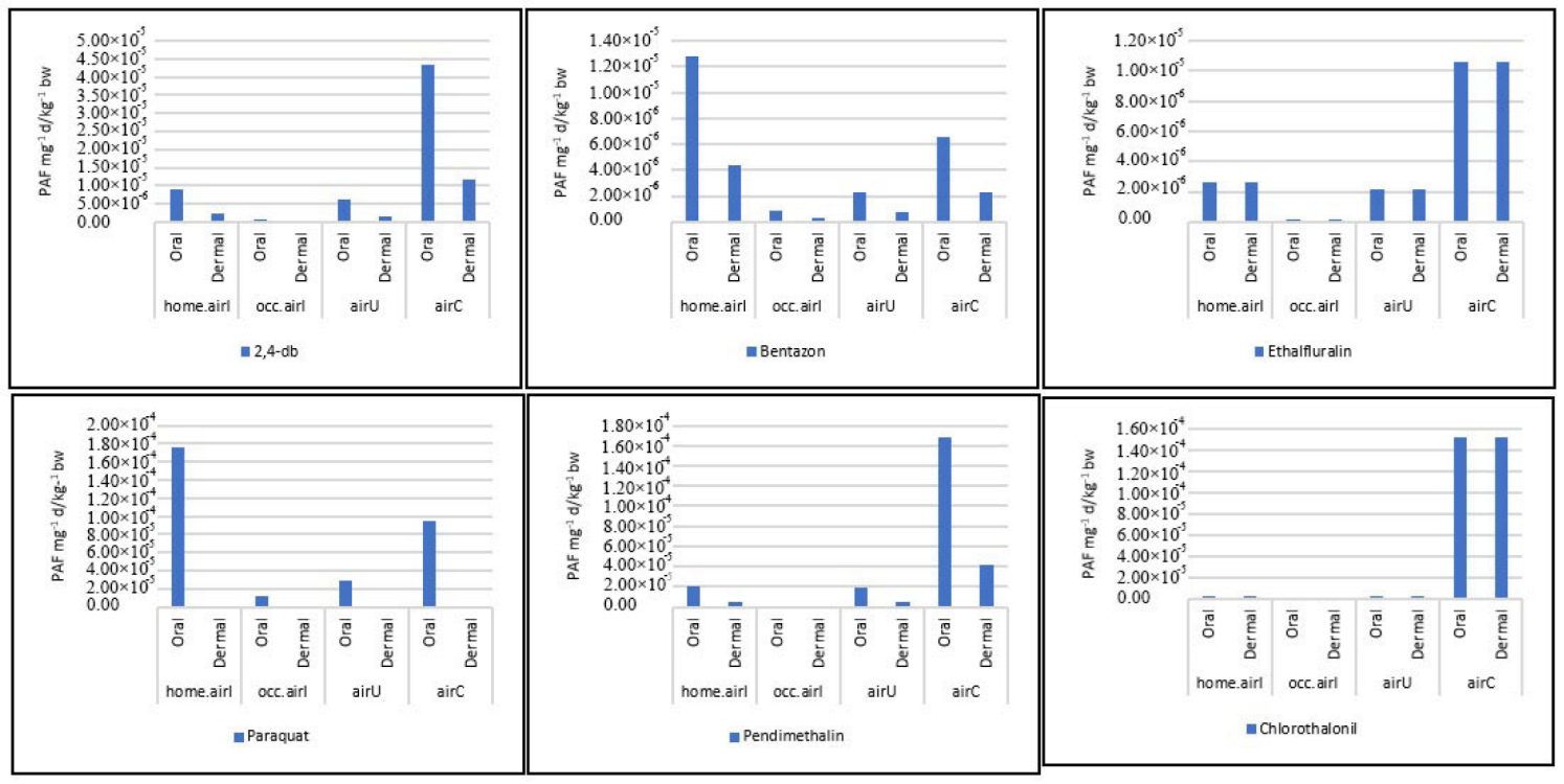
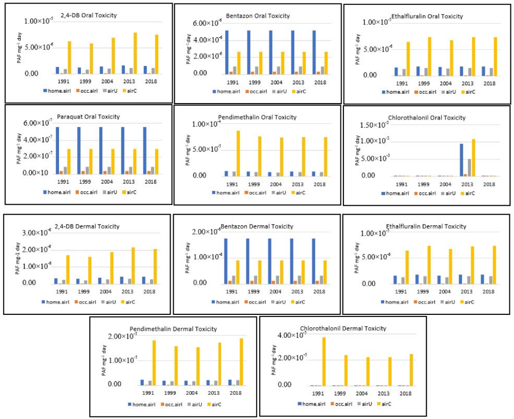
3.5. Potential Oral and Dermal Toxicity of the Six Common AIs (End-Point)

Ethalfluralin, 2,4-DB, and Pendimethalin had a higher oral impact in continental air than other air scales. In comparison, Bentazon and Paraquat’s oral impact in-home air was higher than on other air scales. Chlorothalonil had a higher impact in 2013 than in other years across all air scales, even though the continental air scale was more elevated in terms of oral impact (Figure 9).

Ethalfluralin, 2,4-DB, Pendimethalin, and Chlorothalonil had a higher dermal impact in continental air than on other air scales, while Bentazon’s oral impact in-home air was higher than on other air scales. The dermal Paraquat effect could not be determined because the LD₅₀ was not found. Given all relevant amounts and processes, this is not a strange or unexpected result; instead, this output allows for factoring out those chemicals for which human or ecological impacts can be considered negligible. In the context of a selected product system, this allows highlighting those compounds for which life cycle choices matter most in terms of human health and ecosystem damage. Appendix A (

Table A1. Oral toxicity potential impact.

AI	2018				2013				2004				1999				1991
	home.airI	occ.airI	airU	airC	home.airI	occ.airI	airU	airC	home.airI	occ.airI	airU	airC	home.airI	occ.airI	airU	airC	home.airI	occ.airI	airU	airC
2,4-DB	1.5 × 10−6	1.0 × 10−7	1.1 × 10−6	7.6 × 10−6	1.6 × 10−6	1.1 × 10−7	1.1 × 10−6	8.0 × 10−6	1.4 × 10−6	9.3 × 10−8	9.8 × 10−7	6.9 × 10−6	1.2 × 10−6	7.8 × 10−8	8.3 × 10−7	5.8 × 10−6	1.3 × 10−6	8.4 × 10−8	8.9 × 10−7	6.3 × 10−6
Bentazon	5.2 × 10−6	3.4 × 10−7	9.3 × 10−7	2.7 × 10−6	5.2 × 10−6	3.4 × 10−7	9.3 × 10−7	2.7 × 10−6	5.2 × 10−6	3.4 × 10−7	9.3 × 10−7	2.7 × 10−6	5.2 × 10−6	3.4 × 10−7	9.3 × 10−7	2.7 × 10−6	5.2 × 10−6	3.4 × 10−7	9.3 × 10−7	2.7 × 10−6
Ethalfluralin	1.8 × 10−6	1.2 × 10−7	1.5 × 10−6	7.4 × 10−6	1.8 × 10−6	1.2 × 10−7	1.5 × 10−6	7.3 × 10−6	1.7 × 10−6	1.1 × 10−7	1.4 × 10−6	6.7 × 10−6	1.8 × 10−6	1.2 × 10−7	1.5 × 10−6	7.4 × 10−6	1.6 × 10−6	1.0 × 10−7	1.3 × 10−6	6.4 × 10−6
Paraquat	5.6 × 10−7	3.7 × 10−8	9.0 × 10−8	3.0 × 10−7	5.6 × 10−7	3.7 × 10−8	9.0 × 10−8	3.0 × 10−7	5.6 × 10−7	3.7 × 10−8	9.0 × 10−8	3.0 × 10−7	5.6 × 10−7	3.7 × 10−8	9.0 × 10−8	3.0 × 10−7	5.6 × 10−7	3.7 × 10−8	9.0 × 10−8	3.0 × 10−7
Pendimethalin	9.4 × 10−6	6.2 × 10−7	8.4 × 10−6	7.5 × 10−5	1.0 × 10−5	6.8 × 10−7	9.2 × 10−6	8.2 × 10−5	9.3 × 10−6	6.1 × 10−7	8.3 × 10−6	7.4 × 10−5	9.5 × 10−6	6.2 × 10−7	8.5 × 10−6	7.6 × 10−5	1.1 × 10−5	7.1 × 10−7	9.7 × 10−6	8.7 × 10−5
Chlorothalonil	4.3 × 10−7	2.8 × 10−8	4.3 × 10−7	2.5 × 10−5	3.9 × 10−7	2.6 × 10−8	3.9 × 10−7	2.2 × 10−5	3.9 × 10−7	2.6 × 10−8	3.9 × 10−7	2.2 × 10−5	4.2 × 10−7	2.7 × 10−8	4.2 × 10−7	2.4 × 10−5	6.5 × 10−7	4.3 × 10−8	6.5 × 10−7	3.7 × 10−5

and

Table A2. Dermal toxicity potential impact.

AI	2018				2013				2004				1999				1991
	home.airI	occ.airI	airU	airC	home.airI	occ.airI	airU	airC	home.airI	occ.airI	airU	airC	home.airI	occ.airI	airU	airC	home.airI	occ.airI	airU	airC
2,4-DB	1.5 × 106	1.0 × 10−7	1.1 × 10−6	7.6 × 10−6	1.6 × 10−6	1.1 × 10−7	1.1 × 10−6	8.0 × 10−6	1.4 × 10−6	9.3 × 10−8	9.8 × 10−7	6.9 × 10−6	1.2 × 10−6	7.8 × 10−8	8.3 × 10−7	5.8 × 10−6	1.3 × 10−6	8.4 × 10−8	8.9 × 10−7	6.3 × 10−6
Bentazon	5.2 × 10−6	3.4 × 10−7	9.3 × 10−7	2.7 × 10−6	5.2 × 10−6	3.4 × 10−7	9.3 × 10−7	2.7 × 10−6	5.2 × 10−6	3.4 × 10−7	9.3 × 10−7	2.7 × 10−6	5.2 × 10−6	3.4 × 10−7	9.3 × 10−7	2.7 × 10−6	5.2 × 10−6	3.4 × 10−7	9.3 × 10−7	2.7 × 10−6
Ethalfluralin	1.8 × 10−6	1.2 × 10−7	1.5 × 10−6	7.4 × 10−6	1.8 × 10−6	1.2 × 10−7	1.5 × 10−6	7.3 × 10−6	1.7 × 10−6	1.1 × 10−7	1.4 × 10−6	6.7 × 10−6	1.8 × 10−6	1.2 × 10−7	1.5 × 10−6	7.4 × 10−6	1.6 × 10−6	1.0 × 10−7	1.3 × 10−6	6.4 × 10−6
Paraquat	5.6 × 10−7	3.7 × 10−8	9.0 × 10−8	3.0 × 10−7	5.6 × 10−7	3.7 × 10−8	9.0 × 10−8	3.0 × 10−7	5.6 × 10−7	3.7 × 10−8	9.0 × 10−8	3.0 × 10−7	5.6 × 10−7	3.7 × 10−8	9.0 × 10−8	3.0 × 10−7	5.6 × 10−7	3.7 × 10−8	9.0 × 10−8	3.0 × 10−7
Pendimethalin	9.4 × 10−6	6.2 × 10−7	8.4 × 10−6	7.5 × 10−5	1.0 × 10−5	6.8 × 10−7	9.2 × 10−6	8.2 × 10−5	9.3 × 10−6	6.1 × 10−7	8.3 × 10−6	7.4 × 10−5	9.5 × 10−6	6.2 × 10−7	8.5 × 10−6	7.6 × 10−5	1.1 × 10−5	7.1 × 10−7	9.7 × 10−6	8.7 × 10−5
Chlorothalonil	4.3 × 10−7	2.8 × 10−8	4.3 × 10−7	2.5 × 10−5	3.9 × 10−7	2.6 × 10−8	3.9 × 10−7	2.2 × 10−5	3.9 × 10−7	2.6 × 10−8	3.9 × 10−7	2.2 × 10−5	4.2 × 10−7	2.7 × 10−8	4.2 × 10−7	2.4 × 10−5	6.5 × 10−7	4.3 × 10−8	6.5 × 10−7	3.7 × 10−5

) provides detailed information on the impact of oral and dermal toxicity.

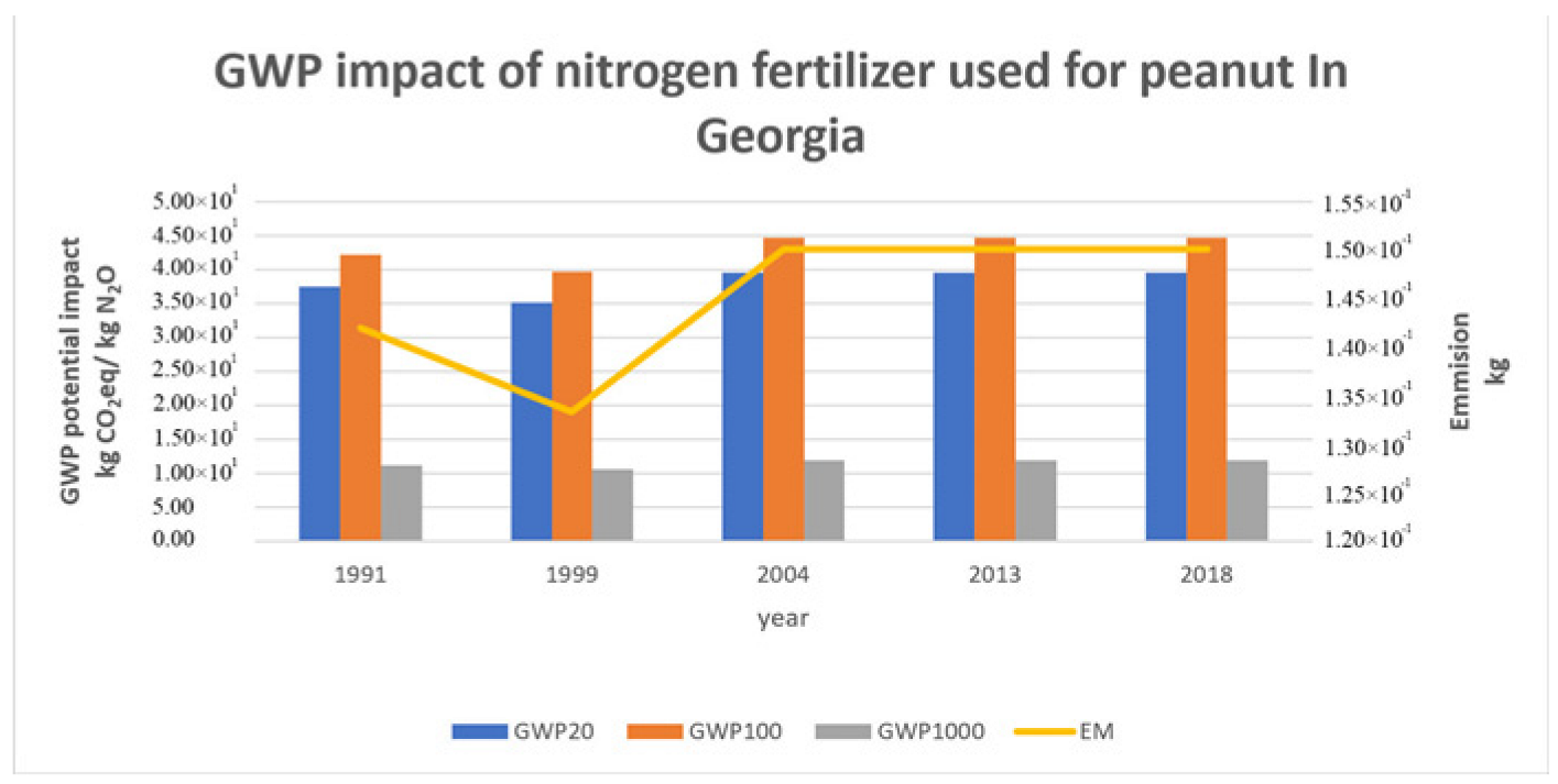
3.6. GWP 20, 100, 1000: Time Horizon of the Fertilizers Used to Produce Peanuts in Georgia (End-Point)

The years 2018, 2013, and 2004 had the same impact because the same amount of nitrogen fertilizer was used. N₂O had a higher GWP impact in the 100-year horizon, followed by the 20-year horizon, because of its short life span.

4. Discussion

In this study, Georgia peanuts were considered as a study case to understand the environmental consequences of fertilizer and pesticide emissions that cause air quality changes and lead to oral and dermal toxicity. Application of the LCA method highlighted that physical and chemical characterization plays a significant role in emission movement and AI reactions. Furthermore, this study provides general information on how pesticide use can affect any surrounding species, not only the targeted one, by analyzing the characteristics of the AIs and their movement through different air scales and how this is related to oral dermal impact. In comparison, other studies focused on one specific species (Weir et al. (2015) on lizards and birds, Amer and Aboul-ela (1985) on mice, Crenna et al. (2020) on honey bees) [47].

4.1. Characterization Factor

As explained above, the CF contains three primary parameters, EF, XF, and FF. According to our observation, the factors that most affected the impact calculations were fate and effect factors. The point of discharge controls the chemical’s fate into the global environment, movements of the atmosphere and the oceans, the rate of exchange processes between the atmosphere and the Earth’s surface, and the rate of chemical loss from various environmental phases [16]. The fate factor combines the chemical’s persistence in the environment (e.g., measured in days) and the relative distribution. Different procedures are critical in determining the fate factor for different substances. The physicochemical properties of the substance decide which processes are most significant for particular contamination. Environmental factors (temperature, rain intensity, etc.) also impact fate and receptor interaction [48]. Mathematically, whenever one of the parameters of a multiplication equation is high, the result will be increased, which is what happened with the CFs of Paraquat, Pendimethalin, and Chlorothalonil. Paraquat had the highest CF among selected AIs only because its EF was high, whereas Pendimethalin had a high CF in contrast. Chlorothalonil had a high CF because of its FF. We did not compare the XF because USEtox set it to 1.00 × ${10}^{+0}$ for consistency only, which was not relevant for ecosystem toxicity. Hence, it is very important to understand what makes the EF and the FF high or low. At the same time, we need to keep in mind the emissions and how the physicochemical properties of the Ais affect it.

The FF is the rate of chemical loss from various environmental phases. The volatilization term expresses the rate of pesticide emission to the air. Volatilization, in which pesticides change from solid/liquid to gas, increases at higher atmosphere layers, can drift to different distances, and can move up to higher altitudes, thousands of kilometers away [49]. The exposure risk, in this case, is mainly for operators, land workers, and people living near the field. Volatilized residues diffuse in the first 0.5 cm of air and are exposed to increasing wind speeds when reaching higher layers in a turbulence process, enhancing the pesticide mixture in the air and exposing the pesticide residues to drifting. This process depends on the physicochemical characteristics of the pesticide, such as vapor pressure, Henrys’ law constant (K_H), solvent composition, soil adsorption capacity, environmental temperature, humidity, wind, and rain. Pesticide molecules with low K_H remain longer in higher air layers and travel long distances, arriving in other continents, such as Antarctica [49]; this explains why most of the selected chemicals had a high oral and dermal impact on the continental air level, except Bentazon and Paraquat, which had high oral and dermal effects in indoor home air. Complex interactions between chemical characteristics and small changes in oral and dermal exposure could explain the variances in these patterns. Vapor pressure, which affects the emission factor, led to Bentazon and Ethalfluralin having the highest emission factors (95%). Van Scoy and Tjeerdema (2014) conducted a study on Chlorthalonil and found out that Chlorthalonil has low values of both Henry’s law and vapor pressure; hence, volatilization losses are limited [50]. That is consistent with our study where 2,4-DB, Pendimethalin, and Chlorothalonil had low K_H and low vapor pressure, indicating that their volatilization losses were limited. Over time, they can travel through the air scales, and the impact on the continental air scale would be higher despite their half-life being low or moderate. Leistra and Van Den Berg (2007) studied Parathion and Chlorothalonil volatilization in a potato crop, initial volatilization was slow due to low vapor pressure, and volatility loss continued over a more extended time period [51]. Ethalfluralin has a high oral and dermal impact on the continental air scale and a high K_H, vapor pressure, and half-life. That is due to many environmental parameters such as plant penetration and phototransformation, leading to a rapid decline in volatilization rate in the first few days after application [51].

On the other hand, Bentazon and Paraquat have a high impact on the indoor home air. Bentazon has a low K_H and a very high emission factor of 95%. Therefore, most of the applied Bentazon is emitted to the air with a high initial volatilization rate, speeding up the transmission process and causing higher oral and dermal exposure in the home air. Paraquat has low K_H and VP; it is used in a low amount and would not build up in the environment and cause a high effect on the continental scale.

The EF for oral exposure is higher in 2,4-DB, Bentazon, and Pendimethalin than for dermal exposure, while the EF of Ethalfluralin and Chlorothalonil was identical for oral and oral dermal exposure. This might be because the LD₅₀ values of 2,4-DB, Bentazon, and Pendimethalin are relatively low for oral exposure (>2000 mg/kg, 2063 mg/kg, and 1250 mg/kg, respectively) but high for dermal exposure (>10,000 mg/kg, >6050 mg/kg, and >5000 mg/kg, respectively). On the other hand, the LD₅₀ values of Ethalfluralin and Chlorothalonil are the same for oral and dermal exposure (>10,000 mg/kg). That is consistent with the rule that a lower LD₅₀ dose indicates a more toxic pesticide. Another reason for these differences could be the vapor pressure. For example, Bentazon is more volatile (vapor pressure: 1.70 × ${10}^{+2}$ mPa at 25 °C) than Ethalfluralin (vapor pressure: $1.20\times {10}^{+1}$ mPa at 25 °C), 2,4-DB (vapor pressure: 8.50 × ${10}^{+0}$ mPa at 25 °C), Chlorothalonil (vapor pressure: 7.60 × ${10}^{-0}$ mPa at 25 °C), and Paraquat (1.30 × ${10}^{-2}$ mPa at 25 °C). The authors of [47] conducted their explement on lizards and birds. They found that the impact of oral exposure was higher than that of dermal exposure. They referred to an increase in volatility from the skin’s surface, which would reduce dermal absorption and toxicity.

4.2. Active Ingredient Characteristics

To better understand the oral and dermal toxicity of the selected AIs, we examined their chemical and physical characterization. The previous section illustrated how the chemical’s vapor pressure and LD₅₀ affect the EF.

Our results showed that the 2,4-DB, Ethalfluralin, and Pendimethalin had a greater oral impact in continental air than on other air scales. In contrast, Bentazon and Paraquat had a greater oral impact on indoor home air than other air scales. Chlorothalonil had a higher impact in 2013 than in other years across all air scales. Ethalfluralin, 2,4-DB, Pendimethalin, and Chlorothalonil had a higher dermal impact in continental air than other air scales. In contrast, Bentazon’s oral and dermal impact in indoor home air was higher than on other air scales. This finding could be related to the AI’s half-life characteristic, which is influenced by vapor pressure and LD₅₀. The half-life is the amount of time it takes for a pesticide to be reduced by half as it fades or degrades in the environment.

After a single half-life, a pesticide will typically break down to 50% of its original level. After two half-lives, only 25% will be left. After three half-lives, about 12% will be left. This process repeats until the residual amount is practically nil. According to Hanson et al. (2015), there are three types of a half-life: low (less than 16 days), moderate (16 to 59 days), and high (over 60 days) [43]. Pesticides with shorter half-lives are less likely to accumulate since they spend less time in the environment. On the other hand, pesticides with longer half-lives are more prone to accumulate after repeated applications [44], which could put neighboring surface water, groundwater, plants, and animals at danger of contamination.

If an AI has a high VP, it will evaporate and break faster; thus, most of the impact would happen in the indoor home air before moving to other air scales. Moreover, if an AI has a short half-life in the soil, it will leach to the air faster and affect home air more than other air scales. For example, Bentazon had the highest vapor pressure among the selected AIs (vapor pressure: 1.70 × ${10}^{+2}$ mPa at 25 °C) and a moderate half-life in the soil of 20 days could explain its higher oral dermal impact in the home air than on other air scales (Figure 10). On the other hand, Ethalfluralin, Pendimethalin, and Chlorothalonil had a low vapor pressure (vapor pressure 1.20 × ${10}^{+1}$, 4.00 × ${10}^{-0}$, and $7.60\times {10}^{-2}$ mPa at 25 °C, respectively) and a longer half-life in the soil of 60 days, 21 days, and 30 days, respectively, which led to a high impact on the continental air scale.

4.3. Potential Uses for This Study

Fertilizer emissions and GWP are important for comparing plant-based and animal-based products. For thousands of years, legumes have been a staple of traditional meals in many world regions. The consumption of legumes per capita has remained relatively constant over the last three decades, whereas meat consumption has increased. Peanut is one of the grain legumes that is a more efficient protein source than animal protein. It does not require the same amount of input per kilogram of protein as animal protein. Because grain legumes can fix nitrogen from the air, only a minimal amount of nitrogen fertilizer is used in their production, which helps the climate profile of these products [52]. Davis et al. (2010) studied meals with different protein sources (same protein, fat, and caloric content) and found that a peanut burger meal emits considerably fewer GHGs than a pork chop meal.

Moreover, ruminant livestock (beef and lamb) has the most significant GHG footprint among major sources of protein, followed by nonruminant livestock (fish, poultry, and pig) and dairy, with legumes and nuts having the lowest [52]. In the future, legumes may be a viable solution to the problem of providing high-quality dietary protein to the world’s growing population. However, this will likely necessitate significant increases in global legume yields, with the majority of legume production being directed toward human consumption rather than livestock feed [53].

On the other hand, understanding the complexities of an AI’s physicochemical properties can help us appreciate the need to apply and maintain pesticide usage guidelines. Since these chemicals have very variable properties and are influenced by various environmental conditions, good practices include selecting the proper time with the right wind speed, temperature, etc. Understanding how various chemicals evaporate can also assist stakeholders in appreciating the structures before and after application, how to wear proper clothing, and how to dispose of the pesticide container according to the label requirements.

Understanding the complexities of an AI’s physicochemical properties can help us appreciate applying and maintaining pesticide usage guidelines because oral and dermal toxicity could contaminate surrounding surface water, groundwater, plants, and animals.

4.4. Key Issues and Recommendations

Because peanut is a legume crop, the primary issue in reducing the influence on air quality is pesticide use rather than nitrogen fertilizers, according to the outcomes. Nitrogen consumption can be improved in arable farming by more precise application, animal husbandry through lower emissions from manure storage and spread, and human nutrition by shifting to a plant-bast protein diet. Land management that enhances the organic content of soils can be used to create a globally significant carbon sink. A second essential concern is good land management, by maintaining soil fertility which accumulates large yields, which are important for the climate and economically efficient agriculture [52].

At the same time, the pesticide consumption impact can be reduced by reading and following the pesticide labels; the benefit can be optimized, and the hazards can be reduced. Applicators should pay close attention to the instructions and any cautionary statements. Pesticide labels carry instructions and limitations. Pesticide labels are legal documents, and using a pesticide in violation of its labeling violates both federal and state laws. The pesticide applicator is legally responsible for the correct application of the pesticide. There are several recommendations to avoid exposure to pesticides: (i) if you inhale pesticide spray or dust, get out of the area as soon as possible; (ii) make use of a closed-loop handling system; (iii) keep personal protective equipment clean and in good condition; (iv) to reduce cutaneous exposure, wash exposed body parts frequently; (v) carefully read pesticide labels.

4.5. Challenges and Limitations

The most significant challenge is ensuring that the approach is appropriate for the covered region and crop. The parameters will change from region to region, and the influence of these parameters will vary from crop to crop, in addition to the physical and chemical qualities of the chemical and environmental variables such as temperature and rain intensity. Another issue is a lack of data; in order to quantify the characterization factors of contaminants, the quantification process is divided into three calculation steps, each of which requires a different factor to be collected and calculated. Lastly, the relationship of these three steps and the calculation results with air emissions and the impact of that process must be established, which could be challenging because of the complexity of LCA. As explained in the USEtox documentation, the CF in USEtox can vary by more than 12 orders of magnitude across chemicals due to (i) vast differences in amounts produced, emitted, and distributed in the environment, (ii) residual masses across different compartments, (iii) fraction taken up by humans and/or ecosystem species, and (iv) differences in species sensitivity to chemical exposure.

4.6. Assumptions Used Future Work

This report sought to provide an overview of the impact of pesticides and fertilizers on air quality. The LCA was the primary model applied, and it is a valuable tool for assessing the life cycle of various products. However, while utilizing LCA, some key assumptions are frequently made that must be considered. The results can give a static representation of reality, which is one of the most significant aspects. Furthermore, the quality of the data may vary greatly across researchers. As a result, outcomes from LCAs should be evaluated with this in mind.

In this study, we made three major assumptions. Firstly, we kept the XF exactly as it was in the USEtox, which was adjusted to 1.00 × ${10}^{+0}$ for consistency only. Secondly, when the number of LD₅₀ showed the > symbol, we increased the values by one. We also used nitrogen fertilizers applied for peanuts as the nitrogen amount in the equation.

There are several areas where further research may be carried out to strengthen the analysis conducted in this study. First, the study’s estimation of pesticide air emissions was based on vapor pressure, neglecting other factors such as spraying practices that could also affect the fate of pesticides after application [33]. Furthermore, this study did not focus on specific species; this paper presented oral and dermal toxicity in general.

5. Conclusions

This study used the LCA method to calculate the oral and dermal toxicity impact from pesticides and the GWP of N₂O from fertilizers used to produce peanuts in Georgia.

The oral and dermal toxicity impact calculation depended on two main factors: emission and characterization factors. In this study, the pesticide’s air emissions were calculated by multiplying the amounts of pesticides applied by their emission factor, which was calculated based on the vapor pressure of the AI of the pesticides. The toxicity characterization factor was calculated by multiplying three parameters: FF, XF, and EF.

As a result of applying the LCA method, 2,4-DB, Bentazon, Chlorothalonil, Ethalfluralin, Paraquat, and Pendimethalin were identified as the commonly used pesticides across the five selected years in Georgia to produce peanuts. Pendimethalin, 2,4-DB, and Chlorothalonil have a higher oral and dermal impact in the continental air than on other air scales because of their low K_H and vapor pressure, indicating they would remain longer in the environment and travel to upper air layers because of the limited volatilization losses. Over time, they would travel to larger air scales, having a greater impact on the continental air scale, despite their low or moderate half-life.

For 2,4-DB, Bentazon, and Pendimethalin, the EF for oral exposure was higher than for dermal exposure, whereas the EF of Ethalfluralin and Chlorothalonil was the same for oral and dermal exposure. These results are a function of the differences in the vapor pressure and LD₅₀ of the AIs. The median lethal dose (LD₅₀) of 2,4-DB, Bentazon, and Pendimethalin was relatively low for oral exposure (>2000 mg/kg, 2063 mg/kg, and 1250 mg/kg, respectively) but high for dermal exposure (>10,000 mg/kg, >6050 mg/kg, and >5000 mg/kg, respectively). On the other hand, the LD₅₀ values for Ethalfluralin and Chlorothalonil were the same for oral and dermal exposure (>10,000 mg/kg). That is consistent with the rule that a lower LD₅₀ indicates a more toxic pesticide. Bentazon has the highest vapor pressure (1.70 × ${10}^{+2}$ mPa at 25 °C) and a 20-day half-life in the soil, which explain why its oral dermal impact in the house air was larger than on other air scales. Ethalfluralin, Pendimethalin, and Chlorothalonil, on the other hand, have a low vapor pressure (vapor pressure: 1.20 × ${10}^{+1}$, 4.00 × ${10}^{+0}$, and 7.60 × ${10}^{-2}$ mPa at 25 °C) and a longer half-life in the soil (60 days, 21 days, and 30 days, respectively), resulting in a large impact on the continental air scale.

The GWP results can be used to compare peanut production in Georgia with other protein sources, which can help with the transition to vegetarianism. However, we need to keep in mind the need for efficient processing of vegetable protein products, such as veggie burgers, because these items are frequently sold frozen due to tiny stock units, resulting in significant energy expenditures for freezing and frozen storage [52].

References

1. Tilman, D.; Balzer, C.; Hill, J.; Befort, B.L. Global Food Demand and the Sustainable Intensification of Agriculture. Proc. Natl. Acad. Sci. USA 2011, 108, 20260–20264. [Google Scholar] [CrossRef] [PubMed] [Green Version]
2. Brandt, K.; Barrangou, R. Applications of CRISPR Technologies across the Food Supply Chain. Annu. Rev. Food Sci. Technol. 2019, 10, 133–150. [Google Scholar] [CrossRef] [PubMed]
3. Arya, S.S.; Salve, A.R.; Chauhan, S. Peanuts as Functional Food: A Review. J. Food Sci. Technol. 2016, 53, 31–41. [Google Scholar] [CrossRef] [PubMed] [Green Version]
4. Settaluri, V.S.; Kandala, C.V.K.; Puppala, N.; Sundaram, J. Peanuts and Their Nutritional Aspects—A Review. Food Nutr. Sci. 2012, 3, 1644–1650. [Google Scholar] [CrossRef] [Green Version]
5. Kiniry, J.R.; Simpson, C.E.; Schubert, A.M.; Reed, J.D. Peanut Leaf Area Index, Light Interception, Radiation Use Efficiency, and Harvest Index at Three Sites in Texas. Field Crops Res. 2005, 91, 297–306. [Google Scholar] [CrossRef]
6. Peanut Country, U.S.A. National Peanut Board. Available online: https://nationalpeanutboard.org/peanut-info/peanut-country-usa.htm (accessed on 31 August 2021).
7. Zain, M.; Si, Z.; Li, S.; Gao, Y.; Mehmood, F.; Rahman, S.-U.; Mounkaila Hamani, A.K.; Duan, A. The Coupled Effects of Irrigation Scheduling and Nitrogen Fertilization Mode on Growth, Yield and Water Use Efficiency in Drip-Irrigated Winter Wheat. Sustainability 2021, 13, 2742. [Google Scholar] [CrossRef]
8. FAO; WFP; IFAD. The State of Food Insecurity in the world—2012. FAO 2012, 5, 65. [Google Scholar]
9. Air and Pesticides. Available online: http://npic.orst.edu/envir/air.html (accessed on 20 October 2021).
10. Impact of Sustainable Agriculture and Farming Practices. Available online: https://www.worldwildlife.org/industries/sustainable-agriculture (accessed on 4 March 2022).
11. Main Sources of Nitrous Oxide Emissions. Available online: https://whatsyourimpact.org/greenhouse-gases/nitrous-oxide-emissions (accessed on 4 March 2022).
12. First Aid—Pesticide Environmental Stewardship. Available online: https://pesticidestewardship.org/homeowner/first-aid/ (accessed on 14 March 2022).
13. Sources of Greenhouse Gas Emissions|US EPA. Available online: https://www.epa.gov/ghgemissions/sources-greenhouse-gas-emissions (accessed on 28 July 2021).
14. US EPA, O. Overview of Greenhouse Gases. Available online: https://www.epa.gov/ghgemissions/overview-greenhouse-gases (accessed on 28 July 2021).
15. Konradsen, F.; van der Hoek, W.; Cole, D.C.; Hutchinson, G.; Daisley, H.; Singh, S.; Eddleston, M. Reducing Acute Poisoning in Developing Countries—Options for Restricting the Availability of Pesticides. Toxicology 2003, 192, 249–261. [Google Scholar] [CrossRef]
16. Yusà, V.; Coscollà, C.; Mellouki, W.; Pastor, A.; de la Guardia, M. Sampling and Analysis of Pesticides in Ambient Air. J. Chromatogr. A 2009, 1216, 2972–2983. [Google Scholar] [CrossRef]
17. Wania, F.; MacKay, D. Peer Reviewed: Tracking the Distribution of Persistent Organic Pollutants. Environ. Sci. Technol. 1996, 30, 390A–396A. [Google Scholar] [CrossRef]
18. Tsai, W.; Cohen, Y.; Sakugawa, H.; Kaplan, I.R. Dynamic Partitioning of Semivolatile Organics in Gas/Particle/Rain Phases during Rain Scavenging. Environ. Sci. Technol. 1991, 25, 2012–2023. [Google Scholar] [CrossRef]
19. Bidleman, T.F. Atmospheric Processes. Environ. Sci. Technol. 1988, 22, 361–367. [Google Scholar] [CrossRef]
20. Atkinson, R.; Guicherit, R.; Hites, R.A.; Palm, W.; Seiber, J.N.; de Voogt, P. Transformations of Pesticides in the Atmosphere: A State of the Art. Water Air Soil Pollut. 1999, 115, 219–243. [Google Scholar] [CrossRef]
21. Muñoz, A.; Vera, T.; Ródenas, M.; Borrás, E.; Mellouki, A.; Treacy, J.; Sidebottom, H. Gas-Phase Degradation of the Herbicide Ethalfluralin under Atmospheric Conditions. Chemosphere 2014, 95, 395–401. [Google Scholar] [CrossRef]
22. US EPA, O. Introduction to Pesticide Labels. Available online: https://www.epa.gov/pesticide-labels/introduction-pesticide-labels (accessed on 25 February 2022).
23. Istriningsih; Dewi, Y.A.; Yulianti, A.; Hanifah, V.W.; Jamal, E.; Dadang; Anugrah, I.S.; Darwis, V.; Sarwani, M.; Mardiharini, M.; et al. Farmers’ Knowledge and Practice Regarding Good Agricultural Practices (GAP) on Safe Pesticide Usage in Indonesia. Heliyon 2022, 8, e08708. [Google Scholar] [CrossRef]
24. US EPA, O. 2,4-D. Available online: https://www.epa.gov/ingredients-used-pesticide-products/24-d (accessed on 25 February 2022).
25. Bentazon. Pesticide Tolerances. Available online: https://www.federalregister.gov/documents/2019/05/01/2019-08785/bentazon-pesticide-tolerances (accessed on 4 March 2022).
26. US EPA, O. Paraquat Dichloride. Available online: https://www.epa.gov/ingredients-used-pesticide-products/paraquat-dichloride (accessed on 1 March 2022).
27. NASD—Pesticide Exposure. Available online: http://nasdonline.org (accessed on 12 November 2021).
28. Lee, K.-M.; Inaba, A. Life Cycle Assessment Best Practices of ISO 14040 Series; Center for Ecodesign and LCA (CEL), Ajou University: Suwon, Korea, 2004; Volume 2004, p. 96. [Google Scholar]
29. Alhashim, R.; Deepa, R.; Anandhi, A. Environmental Impact Assessment of Agricultural Production Using LCA: A Review. Climate 2021, 9, 164. [Google Scholar] [CrossRef]
30. Weather-Us, Georgia, USA—Climate Data and Average Monthly Weather. Available online: https://www.weather-us.com/en/georgia-usa-climate (accessed on 28 October 2021).
31. Fertilizer 101: The Big 3—Nitrogen, Phosphorus and Potassium. Available online: https://www.tfi.org/the-feed/fertilizer-101-big-3-nitrogen-phosphorus-and-potassium (accessed on 3 December 2021).
32. Yang, Y. Life Cycle Freshwater Ecotoxicity, Human Health Cancer, and Noncancer Impacts of Corn Ethanol and Gasoline in the U.S. J. Clean. Prod. 2013, 53, 149–157. [Google Scholar] [CrossRef]
33. Peña, N.; Knudsen, M.T.; Fantke, P.; Antón, A.; Hermansen, J.E. Freshwater Ecotoxicity Assessment of Pesticide Use in Crop Production: Testing the Influence of Modeling Choices. J. Clean. Prod. 2019, 209, 1332–1341. [Google Scholar] [CrossRef]
34. Corrado, S.; Castellani, V.; Zampori, L.; Sala, S. Systematic Analysis of Secondary Life Cycle Inventories When Modelling Agricultural Production: A Case Study for Arable Crops. J. Clean. Prod. 2018, 172, 3990–4000. [Google Scholar] [CrossRef]
35. Gentil, C.; Basset-Mens, C.; Manteaux, S.; Mottes, C.; Maillard, E.; Biard, Y.; Fantke, P. Coupling Pesticide Emission and Toxicity Characterization Models for LCA: Application to Open-Field Tomato Production in Martinique. J. Clean. Prod. 2020, 277, 124099. [Google Scholar] [CrossRef]
36. Ministry of Agriculture. Food and Fisheries, B.C. Pesticide Toxicity and Hazard. 2/2022, 9. Available online: https://www.cabdirect.org/cabdirect/abstract/19631802537 (accessed on 14 March 2022).
37. Corporation (SAIC), S.A.I.; Curran, M.A. Life-Cycle Assessment: Principles and Practice 2006. Available online: people.cs.uchicago.edu/~ftchong/290N-W10/EPAonLCA2006.pdf (accessed on 14 March 2022).
38. Huijbregts, M. Uncertainty and Variability in Environmental Life-Cycle Assessment. Int. J. Life Cycle Assess. 2002, 7, 173. [Google Scholar] [CrossRef] [Green Version]
39. Bare, J. TRACI 2.0: The Tool for the Reduction and Assessment of Chemical and Other Environmental Impacts 2.0. Clean Technol. Environ. Policy 2011, 13, 687–696. [Google Scholar] [CrossRef]
40. US EPA, O. Pesticide Volatilization. Available online: https://www.epa.gov/reducing-pesticide-drift/pesticide-volatilization (accessed on 1 December 2021).
41. Hanson, B.; Bond, C.; Buhl, K.; Stone, D. Pesticide Half-Life Fact Sheet. Available online: http://npic.orst.edu/factsheets/half-life.html (accessed on 10 January 2022).
42. Pesticide Vapor Pressure. Available online: http://npic.orst.edu/factsheets/vaporpressure.html (accessed on 30 November 2021).
43. van de Meent, D.; Huijbregts, M.A.J. Calculating Life-Cycle Assessment Effect Factors from Potentially Affected Fraction-Based Ecotoxicological Response Functions. Environ. Toxicol. Chem. 2005, 24, 1573–1578. [Google Scholar] [CrossRef] [PubMed]
44. Weir, S.M.; Yu, S.; Talent, L.G.; Maul, J.D.; Anderson, T.A.; Salice, C.J. Improving Reptile Ecological Risk Assessment: Oral and Dermal Toxicity of Pesticides to a Common Lizard Species (Sceloporus Occidentalis). Environ. Toxicol. Chem. 2015, 34, 1778–1786. [Google Scholar] [CrossRef]
45. Amer, S.M.; Aboul-ela, E.I. Cytogenetic Effects of Pesticides: III. Induction of Micronuclei in Mouse Bone Marrow by the Insecticides Cypermethrin and Rotenone. Mutat. Res. Toxicol. 1985, 155, 135–142. [Google Scholar] [CrossRef]
46. Crenna, E.; Jolliet, O.; Collina, E.; Sala, S.; Fantke, P. Characterizing Honey Bee Exposure and Effects from Pesticides for Chemical Prioritization and Life Cycle Assessment. Environ. Int. 2020, 138, 105642. [Google Scholar] [CrossRef]
47. Fantke, P.; Bijster, M.; Hauschild, M.Z.; Huijbregts, M.; Jolliet, O.; Kounina, A.; Magaud, V.; Margni, M.; McKone, T.E.; Rosenbaum, R.K.; et al. USEtox® 2.0 Documentation (Version 1.00); USEtox® Team: Lyngby, Denmark, 2017; ISBN 978-87-998335-0-4. [Google Scholar] [CrossRef]
48. Langenbach, T.; Caldas, L.Q. Strategies for Reducing Airborne Pesticides under Tropical Conditions. Ambio 2018, 47, 574–584. [Google Scholar] [CrossRef]
49. Van Scoy, A.R.; Tjeerdema, R.S. Environmental Fate and Toxicology of Chlorothalonil. In Reviews of Environmental Contamination and Toxicology Volume 232; Whitacre, D.M., Ed.; Reviews of Environmental Contamination and Toxicology; Springer International Publishing: Cham, Switzerland, 2014; pp. 89–105. ISBN 978-3-319-06746-9. [Google Scholar]
50. Leistra, M.; Van Den Berg, F. Volatilization of Parathion and Chlorothalonil from a Potato Crop Simulated by the PEARL Model. Environ. Sci. Technol. 2007, 41, 2243–2248. [Google Scholar] [CrossRef]
51. Deer, H.M. Pesticide Adsorption and Half-Life. AG/Pestic. 1999, 15, 1. [Google Scholar]
52. Sonesson, U.; Davis, J.; Ziegler, F. Food Production and Emissions of Greenhouse Gases: An Overview of the Climate Impact of Different Product Groups; SIK Institutet for Livsmedel och Bioteknik: Göteborg, Sweden, 2010; ISBN 978-91-7290-291-6. [Google Scholar]
53. Semba, R.D.; Ramsing, R.; Rahman, N.; Kraemer, K.; Bloem, M.W. Legumes as a Sustainable Source of Protein in Human Diets. Glob. Food Secur. 2021, 28, 100520. [Google Scholar] [CrossRef]
Figure 1. The increasing vegetarianism worldwide [26,27,28].
Sustainability 14 03671 g001
Figure 2. Overview of life cycle assessment (LCA) phases.
Sustainability 14 03671 g002
Figure 3. Overview of phase 1 (goal and scope definitions) for the current study.
Sustainability 14 03671 g003
Figure 4. Overview of phase 2 (life cycle inventory) for fertilizers and pesticides in the current study.
Sustainability 14 03671 g004
Figure 5. Flowchart showing the process of selecting the included AIs of the pesticides.
Sustainability 14 03671 g005
Figure 6. Overview of phase 3 (life cycle impact assessment) for the current study.
Sustainability 14 03671 g006
Figure 7. Overview of phase 4 (life cycle interpretation) for the current study.
Sustainability 14 03671 g007
Figure 8. CFs of the six common AIs (midpoint).
Sustainability 14 03671 g008
Figure 9. Potential oral and dermal toxicity of the six common AIs (endpoint).
Sustainability 14 03671 g009
Figure 10. GWP impact of nitrogen fertilizer used for peanut in Georgia (endpoint).
Sustainability 14 03671 g010