Article

A Clustering Spatial Estimation of Marginal Economic Losses for Vegetation Due to the Emission of VOCs as a Precursor of Ozone

School of Economics and Trade, Guangdong University of Foreign Studies, Guangzhou 510006, China
Sustainability 2022, 14(6), 3484; https://doi.org/10.3390/su14063484
Submission received: 3 February 2022 / Revised: 11 March 2022 / Accepted: 14 March 2022 / Published: 16 March 2022

Abstract

:
The economic losses of vegetation caused by ozone were usually evaluated with existing ozone concentrations. However, in the case a new project is assessed, the marginal losses induced by the additional emissions of ozone’s precursors are required. As ozone is VOC-sensitive in China, this study used novel approaches to assess the marginal economic losses (MELs) for vegetation due to the emission of VOCs as a precursor of ozone, which integrated the geographically constrained AHC algorithm with the spatial regression and applied the cluster-specific coefficients of VOC emissions to the MEL estimation. The new approaches reduce the regression sigma2 from 94.5 to 64.6. The marginal contributions of VOC emissions to ozone concentrations range from 0.123 to 1.180 μg/m3 per kilotonne of emissions per year per 0.25 × 0.25 degree. Negative marginal contributions of NOx emissions were found in Southeast China and the Yunan Guizhou Plateau. County-level marginal increases in AOT40s and MELs due to VOC emissions for crops, semi-natural products, and coniferous and deciduous forests were presented as maps. These values are exceedingly large in Northeast China and the Yunan Guizhou Plateau. Due to the high timber prices, sensitivities to ozone, and long growing seasons, MELs of forests are higher than those of other vegetation types, and thus factories with VOC emissions should be away from the surrounding areas of forests.

1. Introduction

Ground-level ozone has become a new threat to human health and vegetation, especially in summer when the chemical reaction between nitrogen oxides (NOx) and volatile organic compounds (VOCs) creates more ozone (O3) in the presence of hot sunlight, in comparison to the relatively heavy particle pollution in winter. The precursors of ozone, NOx and VOCs, are major anthropogenic emissions increasing with the growth of the economy, leading to the wide spreading of ozone. Asia has emerged as the continent with the highest ozone levels, and several regions of China have been identified as places where ozone is likely to jeopardize food supply and ecosystems [1]. Ozone causes damage to plants by affecting the respiration of leaves and oxidizing the tissue around stomata. The damage and related economic losses caused by the existing ozone concentrations have been assessed for the Yangtze River Delta [2,3], Southern China [4], and China [5]. These studies are based on ozone concentrations. In contrast to these studies, the purpose of this paper is to find out the relationship between the additional (marginal) emissions of ozone’s precursors and the damage or loss caused, as ozone, formed by the photochemical reaction mentioned above, is not directly emitted from sources. Consequently, to assess a new project that induces new emissions, in the relationship between emissions and damage, the emissions of its precursors instead of those of ozone should be used. That is, by changing from concentrations to emissions, the damage or loss study has to consider ozone–NOx–VOC sensitivities. With regard to precursors, there are two options, NOx and VOCs. As suggested by existing studies [6,7,8], VOCs play a more critical role in controlling ozone concentrations in China. Therefore, both precursors were checked in our study with a focus on VOCs.
VOCs have been identified as a major pollutant that contributes to the ground-level ozone by the Chinese Ministry of Ecology and Environment, and a comprehensive treatment scheme was proposed to manage the VOC emissions in key industries, i.e., the petrochemical industry, chemical industry, industrial coating, packaging and printing industry, and oil storage and transportation. It was found that in certain countries, large increases in ozone concentrations are generated when industries are located far away from NOx emission sources and near to natural VOC emissions [9]. In most urban areas of China, ozone is VOC-sensitive [7], such as Lanzhou [8] and Chengdu and Chongqing [6]. Therefore, VOC emissions in these areas create a high ozone level which could damage vegetation including agricultural crops and natural plants and induce economic losses. However, most existing studies did not evaluate the vegetation losses caused by VOC emissions, only the losses caused by ozone concentrations. As for China, it was found that relative yield losses, induced by existing ozone concentrations, ranged from 6% to 36.05% for wheat and 4.9% to 23.87% for rice [2,3,4,5], and the corresponding economic losses of wheat and rice are USD 11.1 billion and 7.5 billion, respectively [5]. The economic losses amount to USD 735 million to 2093 million for wheat and USD 1037 million to 2370 million for rice [2,3] in the Yangtze River Delta and USD 108 million to 486 million for rice in Southern China [4]. Ozone was estimated to create yield losses of 18% to 21% for soybean, yield losses of 1.9% to 7.2% for corn, and biomass losses of 11% to 13% for forests in China [5,10,11], yield losses ranging from 7% to 26% for wheat in Mexico [12], 4% to 48% yield losses for various vegetation types in the Kanto region of Japan [13], and 20% to 31% worldwide yield losses for the grape [14]. Other studies assessed the effects of ozone on the yields of oilseed rape [15], cotton [16], and semi-natural vegetation [17,18]. In the Kanto region, crops were found to be most sensitive to ozone levels with a maximum yield reduction of 40% [13].
Study of the relationship between VOC emissions and vegetation losses is more difficult than that between ozone concentrations and vegetation losses because emission study involves ozone–VOC–NOx sensitivities and the complicated compounds in VOCs [19]. As mentioned above, it is suggested that ozone levels are sensitive to VOCs in Chinese urban areas. This is not always true. Ozone is believed to be NOx-sensitive in south European regions [20] and in Delhi, India [21]. Generally, a specific mixing ratio of NOx and VOCs produces a high ozone concentration [21]. Taking account of these facts, in this study, both NOx and VOC emissions were considered in our model, and NO2 concentrations were used in the clustering, as well as the meteorological conditions and topographic factors. The same VOC emission could produce different levels of ozone depending on the NOx concentrations, weather conditions such as solar radiation, wind, precipitation, and relative humidity, and topographic features such as elevation and slope.
In addition, most air pollutants are spatially correlated [22,23]; to evaluate the marginal contribution of VOC emissions to ozone levels more accurately, the spillover effects of the neighboring areas should be controlled. In other words, the background ozone concentrations have to be excluded from the assessment of the effects of local emissions. Hence, in this study, the spatial regression with a spatial weight matrix, which represents the distances between locations, was used to evaluate the marginal effects of local VOC emission on ozone levels. To summarize, the accurate estimation of marginal losses caused by VOC emissions requires an integrated solution to the following questions: (i) How to differentiate the effects of local emissions from the dispersion effects of neighboring emissions? (ii) Do the effects (coefficients) of the emissions on ozone concentrations vary significantly across geographic regions with different meteorological and topographic features? (iii) How to integrate the existing satellite data, monitoring data, emission data, and land cover data for the purpose? (iv) In terms of marginal economic losses, are there significant disparities between regions and between vegetation types? To answer these questions, in the following sections, we introduce relevant data, methods, results, discussion, and conclusions.

2. Materials and Methods

2.1. Data

Data from 2015 were used in our study due to the availability of county-level statistics. Sampling points included 1493 monitoring station points, after removing four stations without ozone monitoring values. These ground-level observed concentrations were sourced from the China Environmental Monitoring Center (CEMC). In the CEMC sample we used, about 4.8% of hourly concentration values were missing, probably due to technical issues or maintenance. In this study, missing values were not patched with arbitrarily determined ones. For stations with missing values, as the clustering and the regression models require only annual mean concentrations, the remaining observed concentrations of the same year were used to calculate annual averages. With regard to the calculation of AOT40s, it was assumed that during the missing hours, the concentrations were below the AOT40 threshold (40 ppb), as the mean ozone concentration is about 27.8 ppb. Because the missing hourly values take up only 4.8% and the AOT40s are calculated for the whole growing seasons instead of individual days with missing values, it is reasonable to believe that the estimated AOT40 values can serve as good indicators. The distribution of ozone concentrations is shown in Figure 1. The circles on the map stand for monitoring stations, and colors inside the circles represent the levels of the observed concentrations. Concentrations were interpolated by the Kriging algorithm to cover areas without monitoring stations. Besides ozone concentrations (variable name: O3), NO2 concentrations (variable name: NO2), used in the clustering algorithm, were also extracted from CEMC.
Emission data came from Multi-resolution Emission Inventory for China (MEIC), and a subset of the finest resolution, 0.25 × 0.25 degree, was used in this study. As explained in the previous section, emissions of both VOCs (VOCEM) and NOx (NOXEM) were used to interpret the ozone levels. The CO emission (COEM) was proven to be positively correlated with ozone [24], and hence its emission values were included in the model. All variables mentioned in this section essentially used values from 2015 to be consistent with the period of the observed concentrations. When values from 2015 were not available, such as GobeLand30, data of the closest year were used.
Meteorological data were employed in both the clustering algorithm and the regression of the ozone concentrations. Meteorological variables were obtained from ERA5. Meteorological variables used in the clustering algorithm consisted of WG (wind gust), SI10 (10 m wind speed), WU10 (10 m u wind component), WV10 (10 m v wind component), T2 (2 m temperature), BLH (boundary layer height), CP (convective precipitation), SP (surface pressure), SSR (surface solar radiation), SSRD (surface solar radiation downwards), TP (total precipitation), and RH (relative humidity). A subset of the above meteorological variables was used in the spatial regression for ozone concentrations, after solving the multicollinearity issue and selecting explanatory variables based on the validation results.
Topographic factors such as DEM (digital elevation model) and SLOPE8K (average slope within 8 km from the sampling point) and a vegetation index such as EVI (enhanced vegetation index) were also used both in the clustering and regression. DEM data were extracted from SRTM (Shuttle Radar Topography Mission), and slopes were calculated based on the DEM data. EVI values were sampled from MODIS (Moderate Resolution Imaging Spectroradiometer), a satellite data source. Distributions of the clustering variables are given in Figure 2. Kaiser–Meyer–Olkin (KMO) values were calculated to assess the adequacy of the clustering variables [25].
Several additional variables were utilized in the spatial regression model, such as the areas of forests and water bodies from GlobeLand30. The areas of forests and water bodies were proven to be important for the prediction of ozone concentrations [26]. In our study, the forest and water areas were aggregated for buffers within 8 km from the sampling points as 8 km was believed to be effective for the estimation of pollutant concentrations [27]. Another explanatory variable for ozone concentrations is the distance to the coast. The distances were calculated based on GIS. Statistical descriptions of variables used in the spatial regression are presented in Table 1, where SK stands for skewness. HS Mode in the table means the half-sample mode, which presents an estimator for the highest-density region of a distribution. Numeric modes become illogical as there are usually multiple modes for these real numbers and each numeric mode has a very low frequency. Moreover, most numeric modes do not correspond to the highest-density regions of these variables. In Table 1, values of EVI, NOXEM, VOCEM, and COEM were divided by 1000, values of SP were divided by 10,000, values of SSR were divided by 1,000,000, and values of TP were multiplied by 1000 to avoid very small or large values. We added 153 to DEM to get positive values (negative DEM values are not in the sampling points).
The county-level marginal yield/biomass losses and marginal economic losses of the vegetation were estimated with data from 2858 counties. County-level areas (within the boundary of a county) of cultivated lands, deciduous forests, coniferous forests, and semi-natural vegetation types were calculated based on land cover data (GlobeLand30) and the 1:1,000,000 vegetation atlas of China. During the estimation of the marginal yield/biomass losses and economic losses, the provincial cultivated land areas, quantities of agricultural products, and market values were obtained from the China Agricultural Statistical Yearbook. The provincial data were used to produce the average yields of different types of lands and the province-specific prices of different products. There are no missing values in meteorological, topographic, provincial, and land cover data.

2.2. Methodology

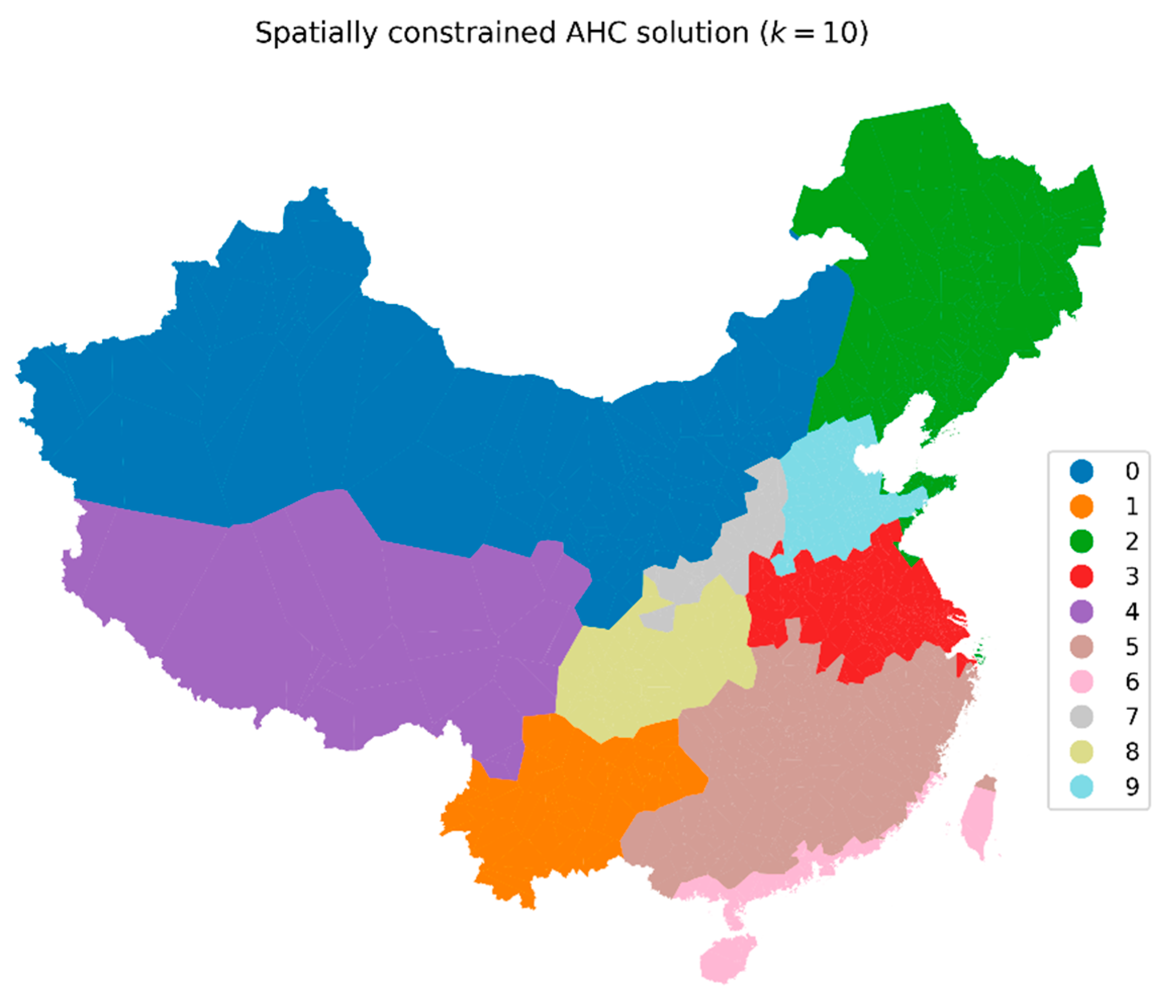
2.2.1. Geographically Constrained Clustering Algorithm

Direct use of a spatial regression model will generate spatially invariable coefficients for the explanatory variables, which is not reasonable considering the spatial heteroscedasticity of the pollution. Another group of regressions, which considers the spatial heteroscedasticity, called geographically weighted regression (GWR), produces variable coefficients for each location. However, the coefficients provided by GWR seem to lack patterns and are too variable to be used, and the marginal estimates from GWR are nearly incomprehensible. However, it was found that GWR works well in health risk assessment [28], which we will discuss in future studies.
An intermediary approach between the two models was proposed in this study, which combines the clustering algorithm and the spatial regression. By validating with the resulting clusters, the geographically constrained agglomerative hierarchical clustering (AHC) was proven to be able to generate realistic results. As a popular clustering algorithm, AHC sequentially combines smaller clusters into larger ones [29]. In this study, geographic constraints were applied in the algorithm to keep the clustering results (called clusters or regimes) geographically continuous, which is required by the spatial regression. The implementation of the geographically constrained AHC algorithm with the Ward linkage is given in Algorithm 1. Y is a set of yi, which in our case denotes a monitoring station with clustering attributes. Ci is a cluster, and RClist keeps a list of the resulting clusters. The Ward linkage minimizes the sum of squared differences within each cluster. The queen type connection means the geographical connection directions are similar to a queen’s movement directions in chess, i.e., moving horizontally, vertically, or diagonally. The number of clusters was set and each attribute z was scaled by (z—mean of z)/(75% quantile of z—25% quantile of z) before the running of the algorithm. To balance the representation of the spatial heteroscedasticity and the sample size within a cluster required to perform an effective spatial regression, 10 was used for the number of clusters by validation. The clustering results were evaluated by Silhouette or Dunn scores [30,31].
Algorithm1. The main part of the geographically constrained AHC algorithm.
  (1) Y = {y1, y2, …, yn}
  (2) Ci = {yi}, for ∀i in 1..n
  (3) For t = Lengh(Y) to NumofClusters step -1
     RClist = {C1, C2, …, Ct}
     d(i, j) = WardDistance(Ci, Cj), ∀i,j in 1…t, i ≠ j, and Ci and Gj are geographically (queen) connected
     p, q = argminx1,x2 d(x1, x2)
     Cp = {Cp} ∪ {Cq}
     Delete Cq from RClist
  (4) Return RClist
The dispersion of pollutants is influenced by weather conditions and terrains; therefore it is natural to include them in the clustering factors. As the effects of VOC emissions on ozone levels depend on whether the study location is in a NOx-sensitive regime (with relatively low NOx and high VOCs) or in a NOx-saturated (VOC-sensitive) regime [32], the concentration of NO2 was added as an important clustering factor in our study. In NOx-saturated regimes, the response of ozone concentrations could negatively relate to NOx emissions and positively correlate with VOCs [6,7]. In NOx-sensitive regimes, mainly in rural areas, where concentrations of NOx are low, concentrations of ozone increase with the increasing NOx emission [8]. Figure 3 gives the scatter plots of the relationships between ozone concentrations and VOC or NOx emissions. In the figure, high ozone levels do not relate to large emissions of VOCs or NOx. After the concentrations of VOCs or NOx become saturated, ozone concentrations tend to be negatively related to additional emissions. Therefore, the concentration of NO2 was added into the clustering variables to reflect the existing levels of NOx and allow a variable coefficient of VOC emissions in response to the NOx levels.

2.2.2. Clustering Spatial Regression

The clustering spatial regression was used to measure the sensitivity of ozone formation to VOC emissions. The marginal change of the ozone concentration caused by a marginal change of VOC emissions in a cluster is indicated by the coefficient of VOC emissions estimated from the clustering spatial regression. Due to the diffusion of air pollutants, it is necessary to use spatial regressions which can capture the spillover effects of pollutants on the adjacent areas. The spatial regression model is appropriate for the estimation of models with spatial correlations of dependent variables or disturbance terms. There are several forms of spatial regression models, such as SAR (spatial autoregressive model), SEM (spatial error model), and SARAR (spatial autoregressive model with spatial error) [33,34]. Correspondingly, three clustering spatial regression models, CSAR (clustering SAR), CSEM (clustering SEM), and CSARAR (clustering SARAR), are presented in this study, shown in Equations (1)–(3), respectively. CSARAR is a combination of CSAR and CSEM. Subscript c is an index for clusters. Clusters are generated from the clustering algorithm. Wc is the spatial weight matrix for cluster c, created by an inverse distance weight function. λc and ρc are the spatial autoregressive coefficients for cluster c. βc is the coefficient vector for cluster c. yc denotes the vector of the dependent variable, i.e., ozone concentrations, in cluster c. εc stands for the disturbance vector of cluster c, and each element in the vector follows iid (independently identically distribution). μc is the error vector including the spatial autocorrelation for cluster c. Xc is a matrix that consists of explanatory variables. The explanation variables include VOC emissions, NOx emissions, CO emissions, EVI, T2, BLH, RH, SP, SSR, TP, DEM, SLOPE8K, WU10, WV10, forest areas within 8 km (FOREST), water body areas within 8 km (WATER), and distances to the coast (SEADIST). The absolute values of WU10 and WV10 were used in the regression. The selection of variables was based on existing studies [26] and cross-validation. As suggested by Elhorst et al., spatial models could be selected based on sigma2 [35], which is the variance of the regression residuals, in addition to the Lagrange multiplier (LM) diagnostic tests for spatial error dependence and spatial lag dependence.
y c = ρ c W c y c + X c β c + ε c
y c = X c β c + μ c ,   a n d   μ c = λ c W c μ c + ε c
y c = ρ c W c y c + X c β c + ε c ,   a n d   μ c = λ c W c μ c + ε c

2.2.3. Estimation of the Marginal Damage to Vegetation

To estimate the marginal damage to vegetation, hourly mean ozone concentrations were converted into AOT40 (accumulated ozone exposure over a threshold of 40 ppb under effective light conditions during the vegetation growing seasons). The conversion was performed with Equation (4) [36]. N is the number of hours included in the growing season. The growing seasons of wheat and rice [10], various types of forests [37], and crops and horticultural plants [36] were sourced from existing studies. It is noteworthy that the growing seasons should be consistent with the slope coefficient β in Equation (5).
AOT 40 = i = 1 N O z o n e i 40   f o r   O z o n e > 40   ppb
The relative yield (RY) was calculated with Equation (5) [4,36]. Y0 is the production without ozone-induced damage, and Y is the production of the vegetation with the losses caused by ozone. The AOT40 in the equation is in ppm h.
RY = Y Y 0 = α + β · AOT 40
The slope coefficient β in the equation stands for the marginal gain/loss of RY caused by a marginal change of the local AOT40. Equation (5) is also called the dose–response function, which measures the relationship between the pollution doze (AOT40) and the response of the production (RY). The coefficients α and β in Equation (5) were obtained from existing studies, and they vary with vegetation types depending on their sensitivity to ozone levels. In our study, we opted to use the coefficients estimated by national studies [10]. When national coefficients were not available, corresponding coefficients from international studies were applied [36,37,38]. It was found that there were no significant differences in the regression coefficients derived from experiments conducted in different countries [36].

2.2.4. Estimation of Marginal Economic Losses

The marginal change of ozone concentrations induced by a marginal emission of VOCs in a county, i.e., the coefficient of the VOC emission, was obtained from the closest monitoring station, and the clustering category of the county was also inherited from that station. The changes of ozone concentrations were converted into the changes of AOT40, which is used in Equation (5) to calculate the marginal gain/loss of the relative yield.
Marginal economic losses, in USD 2015, were estimated based on the marginal yield losses of crops or biomass losses of forests and semi-natural products by multiplying them by their prices. The prices of the corresponding crops or forest products, in RMB 2015, were obtained by dividing the total output values by the total quantity, both from the China Agricultural Statistical Yearbook. The annual average currency exchange rate from RMB to USD was from the Chinese Statistical Yearbook.

3. Results

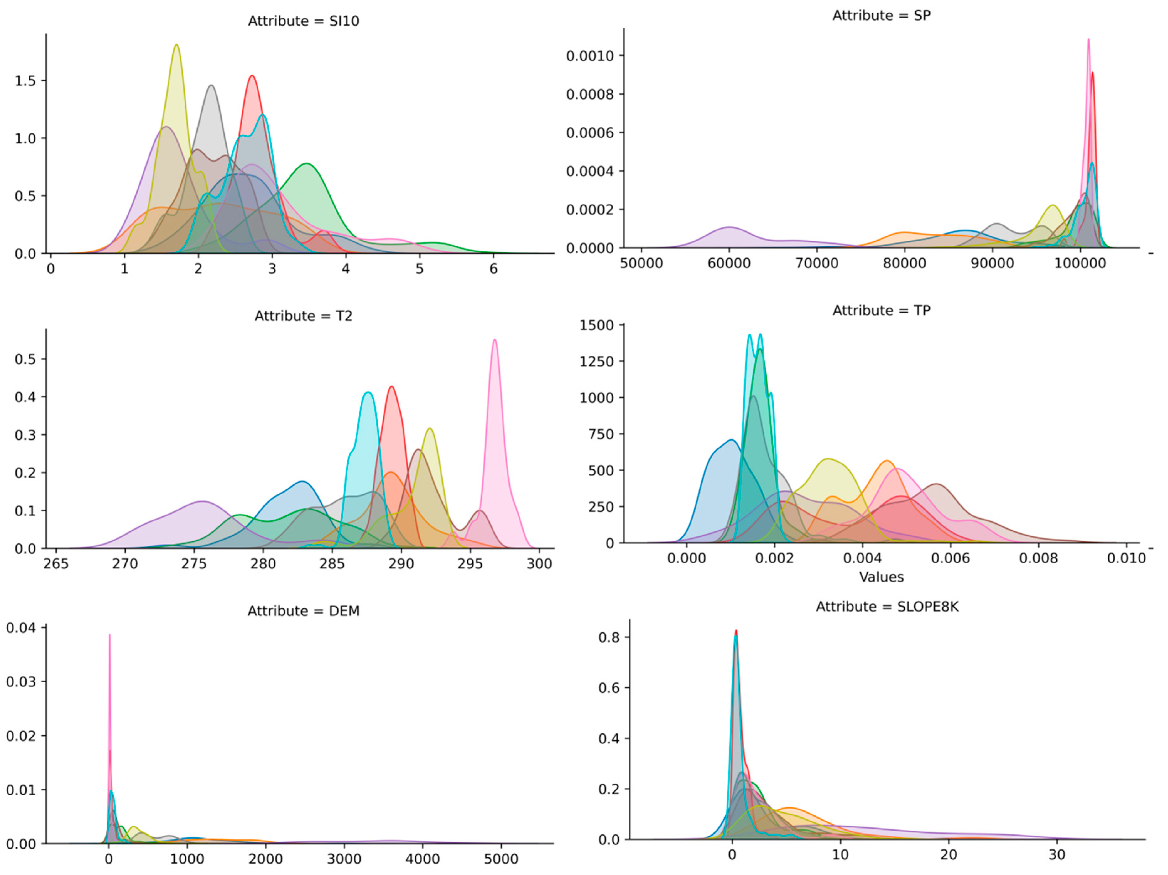
3.1. Clustering Results

The results of the clustering algorithm are illustrated in Figure 4. The clustering algorithm automatically recognizes the regional characteristics of meteorological factors, topographic features, and NO2 concentrations. Resulting clusters reflect the climatic type distribution and topographic characteristics in China, including Northwest China (cn = 0, cn is the serial number of a cluster), the Yunnan Guizhou Plateau (cn = 1), Northeast China (cn = 2), the Jianghuai Region (cn = 3), the Qinghai–Tibet Plateau (cn = 4), Southeast China (cn = 5), the southeast coastal cluster (cn = 6), the Shanxi–Shaanxi Basin (cn = 7), the Sichuan Basin (cn = 8), and the Huabei Plain (cn = 9). As the clusters are automatically generated by the algorithm, the boundaries of the clusters named above are not strictly consistent with the boundaries of the same geographic name areas. Since there are no clear topographic or meteorological boundaries between the Jianghuai Region and the Huabei Plain, the division between these two clusters is mainly caused by the concentrations of NO2. By removing NO2 from the clustering variables, these two clusters will be combined into one.
The Silhouette score for the clustering is 0.15. In contrast with a normal clustering which can freely adjust the parameters to get a perfect clustering, the clustering in this study, however, is fused with the spatial regression, and more stress is the accuracy of the regression as it produces the marginal contribution of emissions to the concentration. Specifically, first, the geographic (connective) constraint is applied to each cluster to generate a reasonable spatial weight matrix for the spatial regression. If we use a k-means clustering without the geographic constraint, the Silhouette score can reach 0.228. Second, the Silhouette score decreases from 0.3917 (cluster number = 2) to 0.15 (cluster number = 8) with the increase in the cluster number and stays around 0.15 when the cluster number is greater than 8. However, if the cluster number is set to 2 to get the largest score of 0.3917, it will cause a lack of variations in concentration–emission sensitivities (only two coefficients obtained from the spatial regressions for the two large clusters). A certain larger cluster number could slightly increase the Silhouette score too, but it causes a lack of enough samples to perform the spatial regression within each cluster, as the number of samples within a cluster decreases with the increasing cluster number. Thus, to balance between the clustering algorithm and the spatial regression, especially to satisfy the requirements of the spatial regression, the cluster number 10 was chosen by iterative validations with different cluster numbers. The current configuration generated realistic clustering results that apparently reflect the meteorological, topographic, and NOx concentration distribution patterns of the country.
The KMO values of the clustering variables are between 0.601 and 0.869, ranging from mediocre ones to meritorious ones, without unacceptable values. The density distributions of the clustering variables for each cluster are shown in Figure 5. It was found that, on average, the Huabei Plain has the highest NO2 concentration, and the Qinghai–Tibet Plateau cluster has the lowest concentration. The lowest average wind speed was found in the Sichuan Basin, whereas the strongest wind is in Northeast China. The highest average temperature is in the southeast coastal cluster, the lowest average temperature in the Qinghai–Tibet Plateau, the highest average humidity in the southeast coastal cluster, and the lowest average humidity in Northwest China. All of the four northern clusters have low precipitation. The solar radiation of the Huabei Plain concentrates in a relatively high value region near 1.3, and thus it tends to accelerate the formation of ozone. In nearly all clusters, elevations and slopes highly concentrate in low-value regions, the surface pressure concentrates in high values, and BLH and EVI concentrate in medium ones.

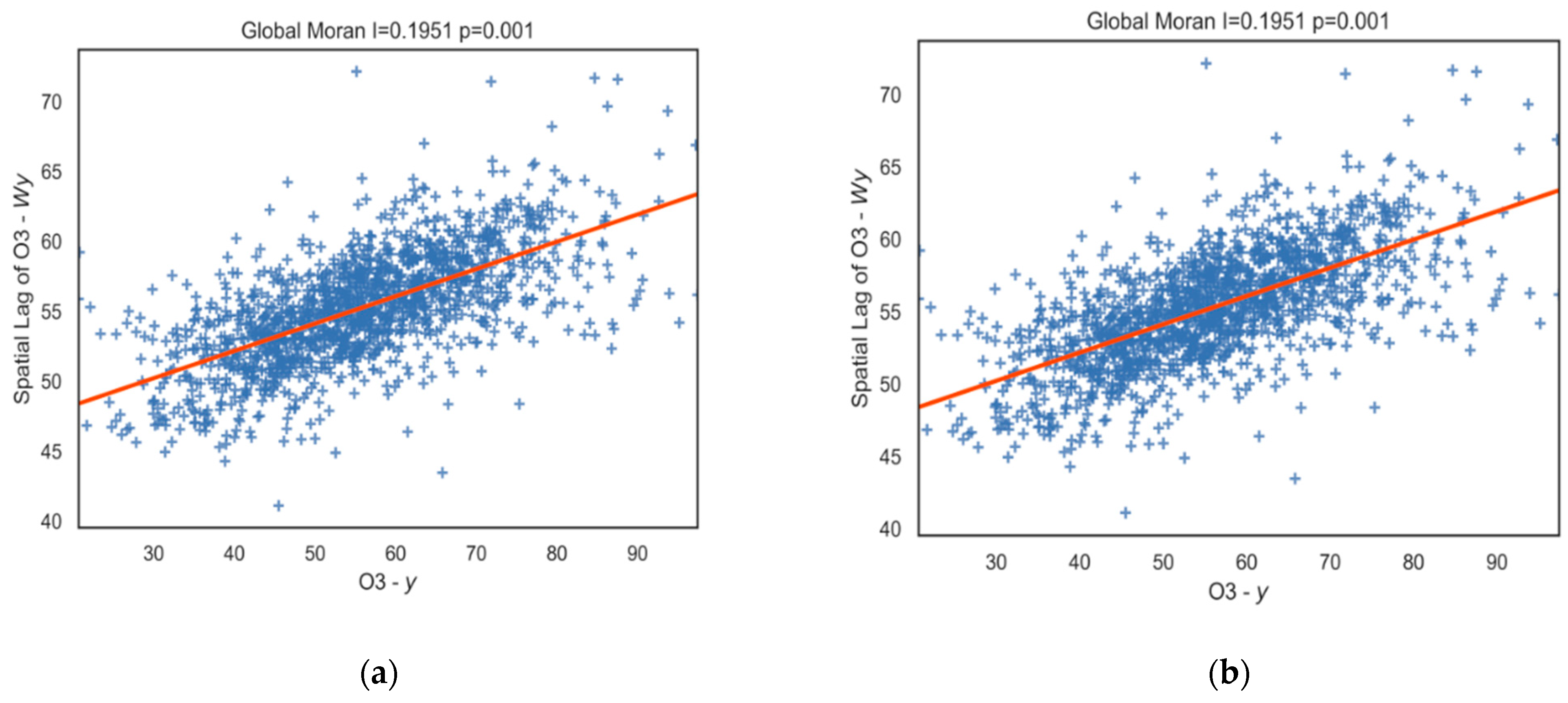
3.2. Spatial Autocorrelation of Ozone Concentrations and OLS Residuals

To determine whether spatial regressions should be used, the Moran’s I tests were performed, and the Moran’s I scatter plots of ozone concentrations and OLS residuals are given in Figure 6a,b, respectively. The statistics of Moran’s I test for global spatial autocorrelation are presented in the titles of the plots. The p values of Moran’s I statistics suggest that both ozone concentrations and OLS residuals are significantly spatially correlated. Therefore, spatial regressions instead of OLS should be used in order to reduce estimation errors.

3.3. Selection of Spatial Models

The Lagrange Multiplier diagnostic tests for spatial error dependence (for SEM) and spatial lag dependence (for SAR) are presented in Table 2. Both the LM test and the robust LMT test significantly reject H0: λSpatial error = 0, but the robust LM test cannot reject H0: ρSpatial lag = 0, indicating that the spatial error dependence is better than the spatial lag dependence, and thus SEM is preferred. This conclusion is checked again by comparing the sigma2 from the spatial regression results in the next step.

3.4. Spatial Regression Results

Regression results of the OLS, SAR, SEM, and SARAR models are given in Table 3. It was found that the emission of VOCs has significantly positive effects on ozone concentrations, and the emission of CO has significantly negative effects on ozone concentrations, whereas the emission of NOx does not significantly affect ozone concentrations. EVI significantly increases ozone concentrations as vegetation emits biogenic VOCs. Temperature reduces ozone concentrations, which is consistent with the ozone concentration map given in Figure 1. The southern parts of China, where the temperature is high, have lower ozone concentrations. SSR significantly increases the level of the ozone as solar radiation takes part in the photochemical formation of ozone. The effect of SSR seems in contradiction to the effect of the temperature as one may think that high SSR occurs in Southern China. However, Figure 5 clearly indicates that the three clusters in the northern parts of China, except Northeast China, have the highest radiation, partially because of the dry and less cloudy weather. North and south wind (v direction) causes more decrease in ozone concentrations than west and east wind (u direction) does. High values of BLH, relative humidity, and surface pressure facilitate the formation of ozone, and ozone concentrations increase with the increase in elevations.
SEM has a regression sigma2 (the bottom row of Table 3) lower than OLS, SAR, and SARAR, which confirms the previous LM test results. The spatial Durbin model and the general Cliff-Ord model were also checked. The general Cliff-Ord model generates a larger sigma2 than that of SEM. The spatial Durbin model produces a similar sigma2 to that of SEM, but it comes with a long list of lagged explanatory variables, which causes multicollinearity. Therefore, the results of SEM are used in the following clustering spatial analysis, and the clustering spatial error regression results are presented in Table 4.
CSEM_0–CSEM_9 indicate the results of cluster 0 to cluster 9. Sigma2s of most clustering spatial regressions are better than those of the global spatial regressions given in Table 3, except cluster 0, the Northwest China cluster with a vast area and a small number of monitoring stations. This implies that the coefficients of the clustering spatial regression are more accurate than those of the global spatial regression. Coefficients of VOC emissions are only significant in several clusters, indicating that the effects of VOC emissions depend on the existence and the level of other precursors such as NO2 and the meteorological and topographic conditions. Following statistical rules, the subsequent estimation of the marginal losses was performed only for clusters with significant coefficients of VOC emissions, which are clusters 1, 2, 3, 5, and 6. The coefficient of cluster 8 (the Sichuan Basin) was also used in the loss assessment as the coefficient of 0.363 is close to the results of an existing sensitivity study for the same region, which is discussed in the next section.
Compared with the significantly positive coefficients of VOC emissions, most coefficients of NOx emissions are not significant, and coefficients of cluster 1 (the Yunnan Guizhou Plateau) and cluster 5 (Southeast China) are even significantly negative, which means lower emissions of NOx create higher ozone levels.
Similar to the global spatial regression, CO emissions are mainly negatively correlated with ozone pollution except in Southeast China. Temperature has negative effects except in the Yunnan Guizhou Plateau. Essentially, in most clusters, BLH, RH, SP, and DEM are positively connected with ozone concentrations. In contrary to the global spatial regression, the clustering spatial regression identifies regions where ozone concentrations are significantly affected by the west and east wind (v direction), such as the southeast coastal cluster, the Jianghuai cluster, and Northwest China, which are either on the east side or on the west side of the country.

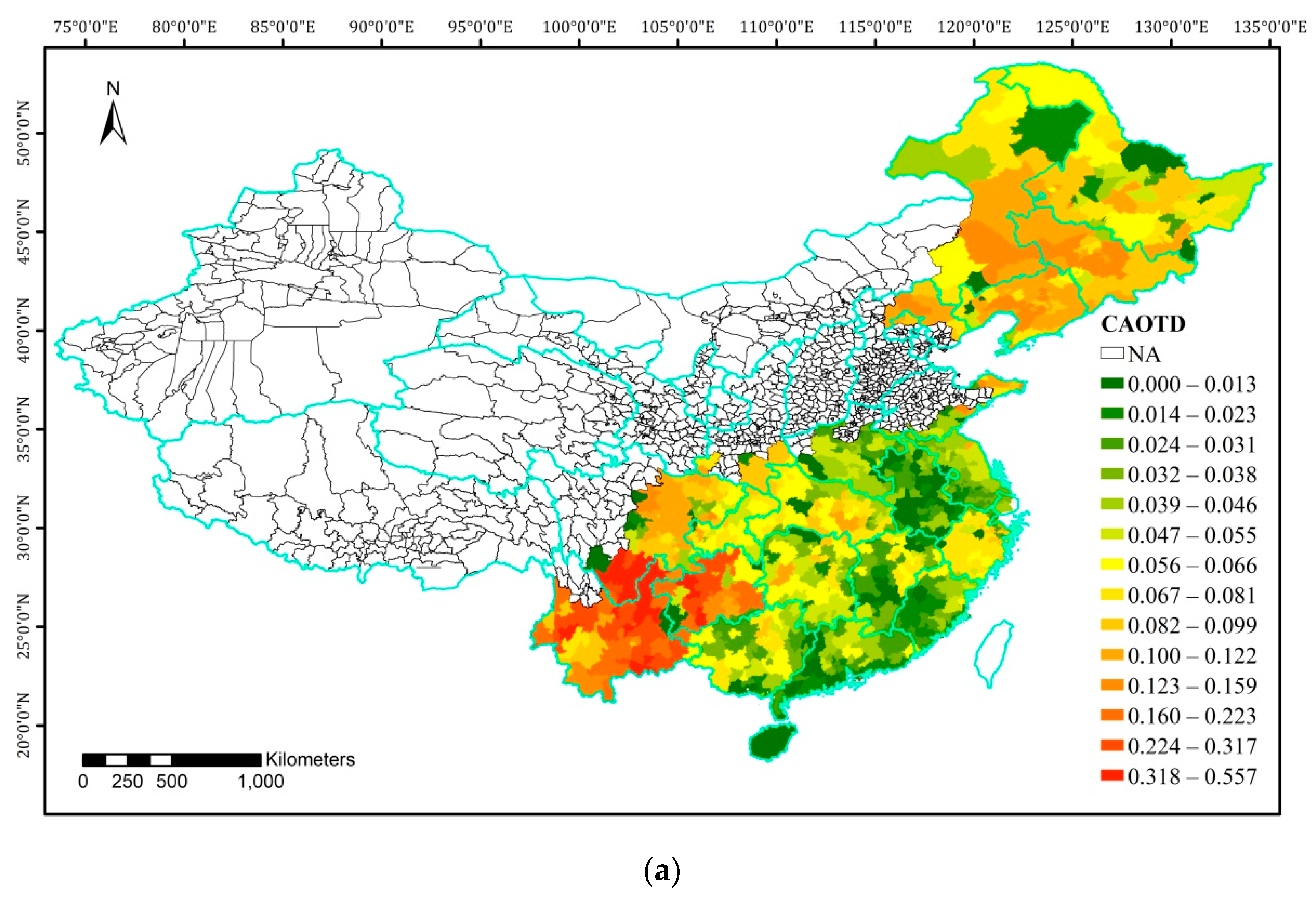
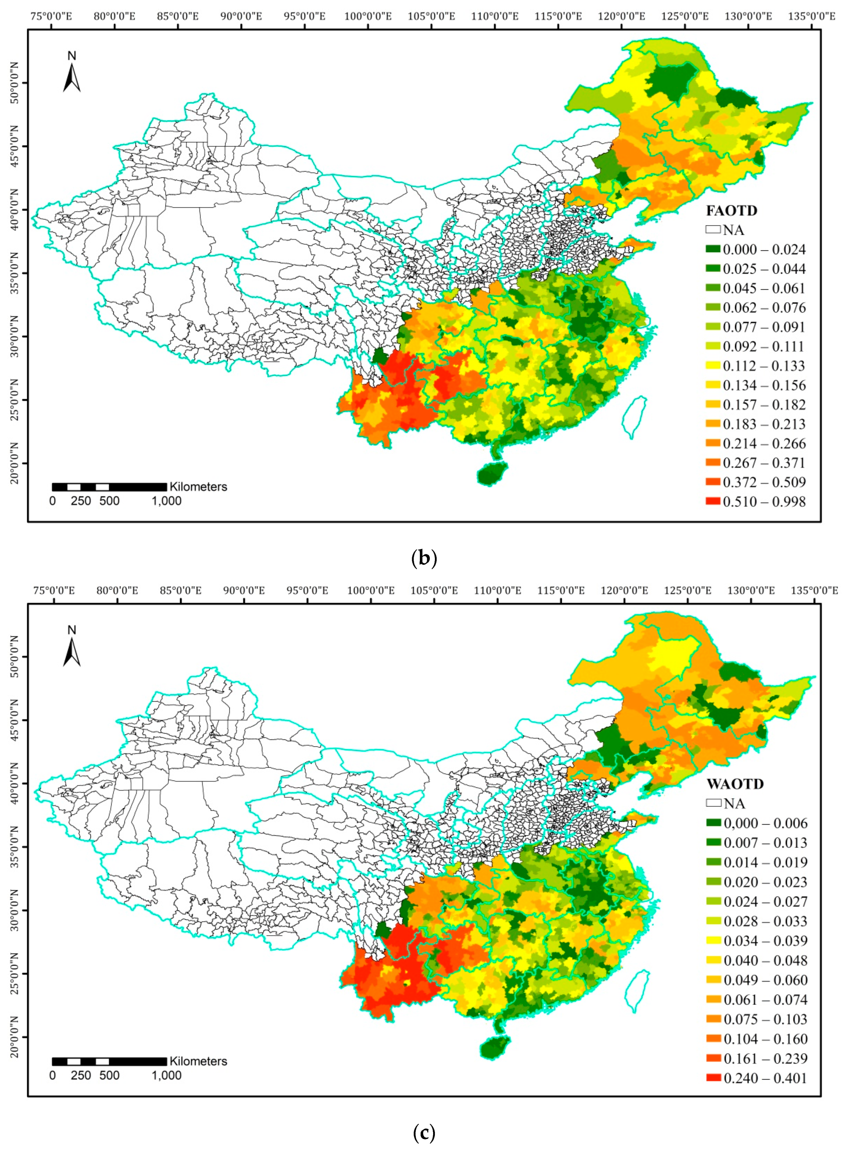
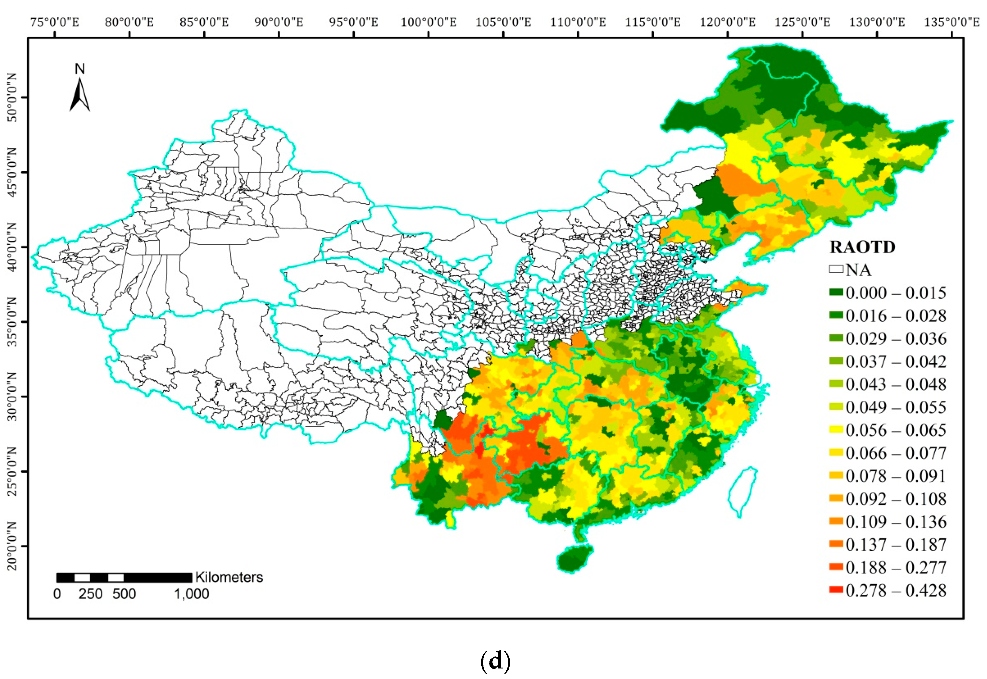
3.5. Changes in AOT40s Caused by the Marginal Emission of VOCs

According to the clustering spatial regression results, the clusters with significant coefficients of VOC emissions and cluster 8 were used in the marginal analysis. The county-level changes of AOT40s caused by a marginal emission of one kilotonne of VOCs are presented in Figure 7, calculated by applying the cluster-specific coefficients and converting from concentrations to AOT40s with Equation (4).
In the calculation of delta AOT40, growing seasons were adjusted according to the vegetation types, resulting in different AOT40 changes for the same county. Hence, Figure 7a–d demonstrate various patterns of distributions. Not all vegetation types are included in Figure 7, such as horticultural vegetation, the distribution of which is similar to that of crops. It was found that additional emission of VOCs induces greater increases in AOT40s in Northeast China and the Yunnan Guizhou Plateau. The growing season of rice is significantly different from the other vegetation types, and this induces relatively large increases in AOT40s in Southeast China.

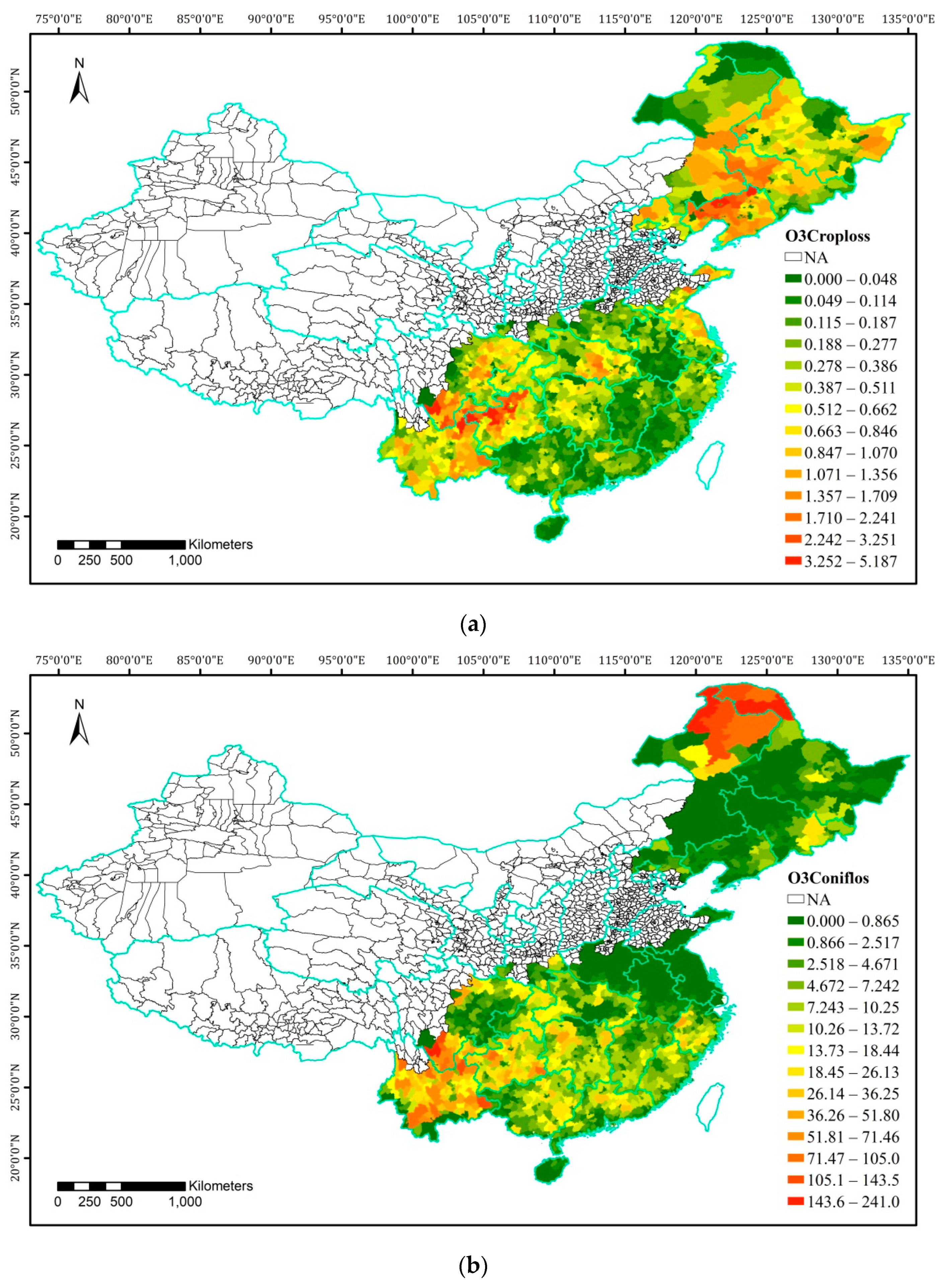
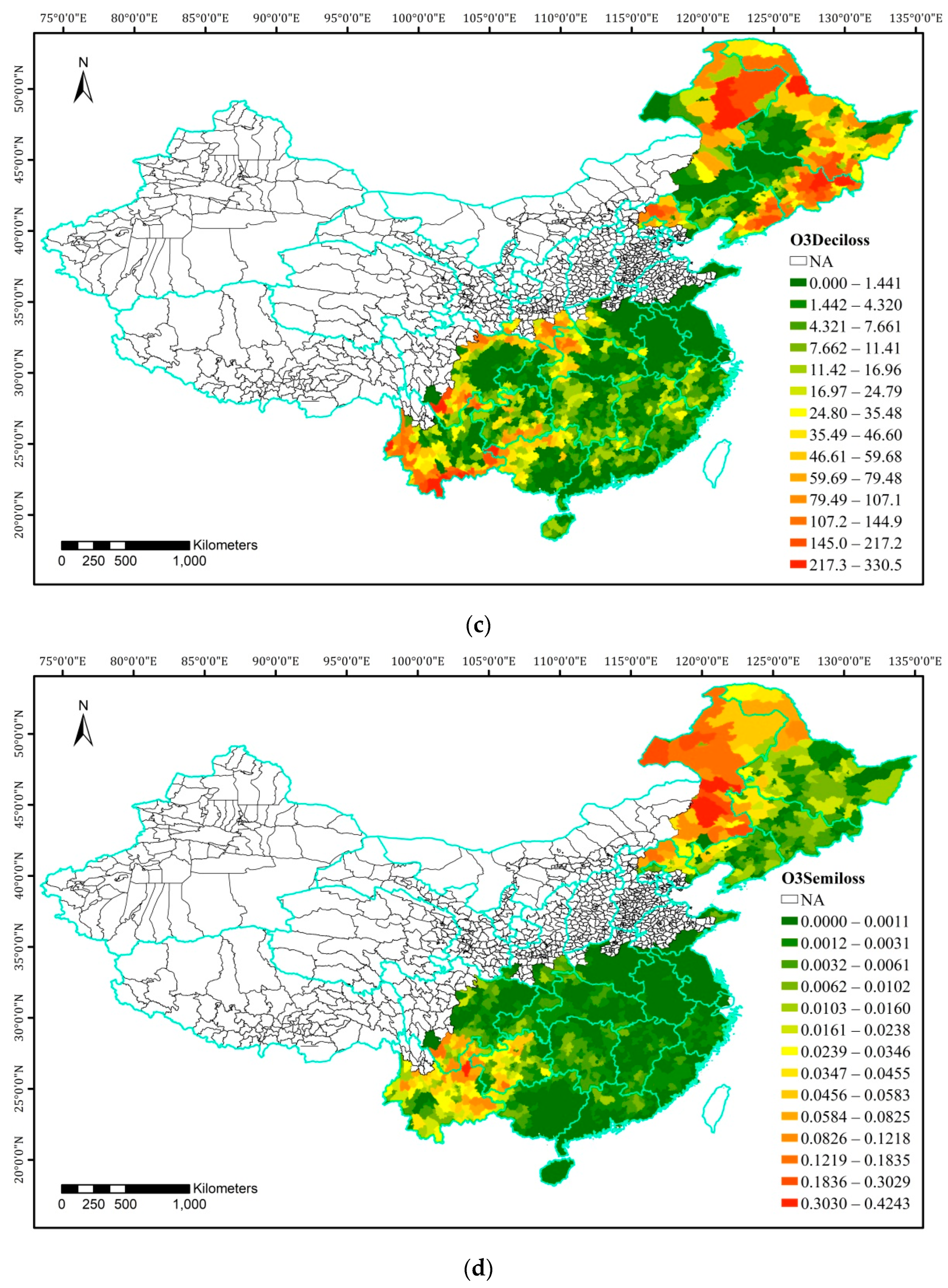
3.6. Marginal Economic Losses Due to the VOC Emission as a Precursor of Ozone

The estimated county-level marginal economic losses (MELs) due to an additional kilotonne of VOC emissions as a precursor of ozone are shown in Figure 8. Values are in USD 2015 K (1000) per year. The values of MELs of a vegetation type depend on the county-level marginal AOT40 changes, county-level distributions and yields of the specific type of vegetation, and the localized prices. For example, MELs of coniferous forests are high in the Greater Khingan Range in Northeast China, where dense coniferous forests are growing, and in the Yunnan Guizhou Plateau, a region with large marginal changes of AOT40s and abundant forest resources. The MELs of coniferous forests range from 0 to USD 241 K per kilotonne of VOC emissions per year per 0.25 × 0.25 degree, as a precursor of ozone.
The MELs of deciduous forests are larger than those of the coniferous forests, ranging from USD 0 to 330.5 K per kilotonne of VOC emissions per year per 0.25 × 0.25 degree, as deciduous forests, with relatively large leaves, are more vulnerable to ozone pollution. In contrast with the coniferous forests, the MELs of deciduous forests are high both in the Greater Khingan Range and in the mountainous areas on the opposite side of Northeast China. MELs of deciduous forests are also high in the Yunnan Guizhou Plateau and the Qinling Mountains.
MELs of semi-natural lands, mainly grasslands, are high in Inner Mongolia, although only a small part of this region was included in the Northeast China cluster. Large areas of grasslands are a striking landscape feature of that region. Another area with high semi-natural economic losses is the Yunnan Guizhou Plateau due to the large marginal increase in AOT40s and abundant vegetation types. The MELs of the semi-natural vegetation range from USD 0 to 0.42 K per kilotonne of VOC emissions per year per 0.25 × 0.25 degree, as a precursor of ozone. Because of the low-value biomass products of the semi-natural vegetation, the MELs are lower than those of forests and crops. Forests have the highest MEL values as their growing seasons are longer than other vegetation types and they are more sensitive to ozone concentrations, in addition to high wood prices.
The MELs of the crops and horticultural products range from USD 0 to 5.19 K per kilotonne of VOC emissions per year per 0.25 × 0.25 degree, as a precursor of ozone. These values are between those of forests and semi-natural products, as growing seasons of crops are shorter than those of forests, and crops are not as sensitive to ozone levels as the forests. The MELs of the crops and horticultural products are high in the Northeast Plain, the eastern parts of the Yunnan Guizhou Plateau, the eastern parts of the Sichuan Basin, the middle reaches of the Yangtze River, and the coastal areas of Northern China.

4. Discussion

This study integrated the clustering algorithm with the spatial regression and clustered the country with variables including the NO2 concentration. Clustering with meteorological and topographic factors significantly reduces the regression square errors, sigma2, from 94.5 to a cluster average of 66.2. The inclusion of NO2 concentrations in the clustering variables further reduces the average sigma2 to 64.6 as the VOC emission reacts differently in NOx-saturated and NOx-sensitive regimes. Density distributions of the clustering variables were presented for each cluster, and this assisted in the explanation of regression results, such as the effects of the high solar radiation in the north and the effects of wind directions. The effect of the v direction wind in the coastal areas is consistent with a study of Shenzhen, a southeast coastal city, where high ozone concentrations are related to the westerly wind [39]. A negative link between NOx emissions and ozone concentrations in the Yunnan Guizhou Plateau and Southeast China was found in this study, which conforms to the existing studies. For example, during the COVID-19 lockdowns, NOx emissions in Wuhan and four European cities decreased by 42–56%, while ozone concentration increased by 17–84% [40,41]. Other studies also found that ozone concentrations are negatively correlated with NOx emission and suggested that the sole control of NOx emissions is not appropriate for the management of ozone pollution [6,42]. In contrast with existing studies, the clustering spatial regression is capable of presenting the variation of NOx emissions’ effects across different clusters.
It is also a novel approach to apply clustering spatial regression coefficients to the marginal loss estimation, which makes the estimation of marginal economic losses of vegetation due to marginal VOC emission as a precursor of ozone more accurate. In addition to the clustering algorithm, this approach considers the spatial correlation of the pollutant and distinguishes the effect of VOC emissions on ozone levels from the diffusion of the ozone from neighboring areas. Hence it ensures that the estimated coefficients represent the pure impacts of local emission and ensures the high accuracy achieved in the marginal loss estimation. Furthermore, the coefficients of VOC emissions were diversified into cluster-specific ones to produce localized marginal changes in ozone concentrations caused by the marginal emission of VOCs.
Our cluster-specific coefficients are close to existing sensitivity results from simulation studies. For example, Cao et al. found that, on average, when VOC emissions decrease by 25%, the ozone concentrations are reduced by 3.1 μg/m3 in the urban area of Chongqing [6]. The average annual emission in the urban areas in Chongqing is 30,944 tonnes (sourced from the MEIC), and thus 3.1/(30,944 ∗ 25%) = 0.0004 μg/m3 per tonne = 0. 4 μg/m3 per kilotonne, close to our coefficient of 0.363 for cluster 8.
Marginal AOT40 changes derived from the marginal concentration changes were performed on an hourly basis to strictly obey the calculation rule of AOT40s and to ensure the accuracy of the estimation of marginal vegetation yield/biomass losses. In the calculation of marginal economic losses, localized areas of crops, forests, and grasslands and local yields and prices for different vegetation types were used to improve the accuracy.
This study identified the counties where emissions of VOCs have significantly positive effects on ozone concentrations. The selected areas shown in Figure 7 and Figure 8 are similar to Cao et al.’s study [4], except that our clusters were automatically generated by the clustering algorithm and selected by the clustering spatial regression, and thus Northeast China was included as a separate region. Our study also identified the counties where large marginal AOT40 changes are created by the same amount of VOC emissions and discerned the counties where marginal yield/biomass losses and marginal economic losses are large due to the marginal emission of VOCs. Usually, these places with large losses have a dense distribution of high-value vegetation, high marginal increases in AOT40s, sensitive yields, and high prices of vegetation products. These county-level marginal loss values could assist in assessing a new project, which may introduce more VOC emissions.

5. Conclusions

Using novel approaches that fused the clustering algorithm with the spatial regression, this study assessed the marginal economic losses of vegetation caused by an additional kilotonne of VOC emissions as a precursor of ozone. Ten clusters were created by the clustering algorithm, which apparently reflect the climatic and topographic distributions of the country. The consideration of the spatial autocorrelation distinguishes the ozone generated by local emissions from the ozone spilled from the neighbors, and the integration of the clustering and the spatial regression significantly reduces the regression sigma2. The clusters with significantly positive coefficients of VOC emissions are mainly in the south part of China and Northeast China. It was found that less NOx emission creates higher ozone levels in Southeast China and the Yunnan Guizhou Plateau. The AOT40 marginal change maps indicate that Northeast China and the Yunnan Guizhou Plateau have the highest increase in AOT40s in response to the marginal emission of VOCs. Aside from that the highest MELs due to the emission of VOCs of semi-natural products occur in Inner Mongolia, MELs are peaking for all other vegetation types in Northeast China and the Yunnan Guizhou Plateau, with exceedingly large MELs for forests in the Greater Khingan Range. In addition to these regions, MELs of crops are prominent in the middle reaches of the Yangtze River, and MELs of deciduous forests are notable in the mountainous areas such as the Qinling Mountains. The soaring MELs of forests are caused by the high prices of timber, the long growing seasons, and the sensitivities of trees to ozone levels.

6. Recommendations

Considering the results found in this study, it is recommended that new factories with VOC emissions should not be placed near the forest areas, especially, avoiding being close to mountainous areas. Large VOC emission sources should be moved out of Northeast China and the Yunnan Guizhou Plateau as the same amount of emissions will produce large AOT40 changes and MELs in these two regions. VOC emission sources should also avoid areas of dense croplands or grasslands, such as the plain areas near the Yangtze River and the Pearl River and Inner Mongolia. In addition to the assessment of the marginal damage to vegetation caused by the emission of VOCs as a precursor of ozone, future studies may evaluate the marginal damage to health induced by the additional VOC emissions to get a full view of marginal losses caused by the VOCs. Alongside the clustering spatial regression, in this case, the geographically weighted regression could be used to discern the more spatial variations and spatial patterns of the health damage and estimate the MELs for health.

Funding

This research was funded by the Humanities and Social Science Foundation of the Ministry of Education of China (Estimation of spatially distributed marginal health damage values of PM2.5 pollution in China, grant number 17YJA790021), the Natural Science Foundation of the Guangdong Province (grant number 2017A030313439), and a special fund from the Institute of City Strategy Studies, Guangdong University of Foreign Studies (grant number JDZB202108).

Data Availability Statement

Data sharing not applicable.

Conflicts of Interest

The author declares no conflict of interest.

References

  1. Emberson, L. Effects of ozone on agriculture, forests and grasslands. Philos. Trans. R. Soc. A 2020, 378, 20190327. [Google Scholar] [CrossRef] [PubMed]
  2. Zhao, H.; Zheng, Y.; Wu, X. Assessment of yield and economic losses for wheat and rice due to ground level O3 exposure in the Yangtze River Delta. China Atmos. Environ. 2018, 191, 241–248. [Google Scholar] [CrossRef]
  3. Ren, X.; Shang, B.; Feng, Z.; Calatayud, V. Yield and economic losses of winter wheat and rice due to ozone in the Yangtze River Delta during 2014–2019. Sci. Total Environ. 2020, 745, 140847. [Google Scholar] [CrossRef] [PubMed]
  4. Cao, J.; Wang, X.; Zhao, H.; Ma, M.; Chang, M. Evaluating the effects of ground-level O3 on rice yield and economic losses in Southern China. Environ. Pollut. 2020, 267, 115694. [Google Scholar] [CrossRef]
  5. Feng, Z.; Marco, A.D.; Anav, A.; Gualtieri, M.; Sicard, P.; Tian, T.; Fornasier, F.; Tao, F.; Guo, A.; Paoletti, E. Economic losses due to ozone impacts on human health, forest productivity and crop yield across China. Environ. Int. 2019, 131, 104966. [Google Scholar] [CrossRef]
  6. Cao, Y.; Li, Z.; Pu, X.; Jiang, C.; Xue, W.; Jiang, H.; Zhang, W.; Zhai, C. Sensitivity of O3 formation from anthropogenic precursor emissions in typical cities in the Chengdu-Chongqing region: A simulation study. Acta Sci. Circumstantiae 2021, 41, 3001–3011. [Google Scholar]
  7. Wang, F.; Wang, J.; Zhai, J.; Hou, C. Emission improvements of reactive VOCs based on satellite observations and their impact on ozone simulations. China Environ. Sci. 2021, 41, 2504–2514. [Google Scholar]
  8. Chen, T.; Wu, M.; Pan, C.; Chang, L.; Li, Y.; Liu, P.; Gao, H.; Hu, A.; Ma, J. Ozone Simulation of Lanzhou City base on Multi-scenario Emission Forecast of Ozone Precursors in the Summer of 2030. Environ. Sci. 2021, 10, 1–14. [Google Scholar]
  9. Castell, N.; Mantilla, E.; Stein, A.F.; Salvador, R.; Millán, M. A Modeling Study of the Impact of a Power Plant on Ground-Level Ozone in Relation to its Location: Southwestern Spain as a Case Study. Water Air Soil Pollut. 2010, 209, 61–79. [Google Scholar] [CrossRef]
  10. Wang, X.; Zhang, Q.; Zheng, F.; Zheng, Q.; Yao, F.; Chen, Z.; Zhang, W.; Hou, P.; Feng, Z.; Song, W.; et al. Effects of elevated O3 concentration on winter wheat and rice yields in the Yangtze River Delta. China Environ. Pollut. 2012, 171, 118–125. [Google Scholar] [CrossRef]
  11. Yi, F.; Feng, J.; Wang, Y.; Jiang, F. Influence of surface ozone on crop yield of maize in China. J. Integr. Agric. 2020, 19, 578–589. [Google Scholar] [CrossRef]
  12. Guarin, J.R.; Emberson, L.; Simpson, D.; Hernandez-Ochoa, I.M.; Rowland, D.; Asseng, S. Impacts of tropospheric ozone and climate change on Mexico wheat production. Clim. Chang. 2019, 155, 157–174. [Google Scholar] [CrossRef]
  13. Shimizu, Y.; Lu, Y.; Aono, M.; Omasa, K. A novel remote sensing-based method of ozone damage assessment effect on Net Primary Productivity of various vegetation types. Atmos. Environ. 2019, 217, 116947. [Google Scholar] [CrossRef]
  14. Blanco-Ward, D.; Ribeiro, A.; Paoletti, E.; Miranda, A.I. Assessment of tropospheric ozone phytotoxic effects on the grapevine (Vitis vinifera L.): A review. Atmos. Environ. 2020, 244, 117924. [Google Scholar] [CrossRef]
  15. Ollerenshaw, J.H.; Lyons, T.; Barnes, J.D. Impacts of ozone on the growth and yield of field-grown winter oilseed rape. Environ. Pollut. 1999, 104, 53–59. [Google Scholar] [CrossRef]
  16. Chaudhary, I.J.; Rathore, D. Effects of ambient and elevated ozone on morphophysiology of cotton (Gossypium hirsutum L.) and its correlation with yield traits. Environ. Technol. Innov. 2022, 25, 102146. [Google Scholar] [CrossRef]
  17. Holder, A.; Hayes, F.; Sharps, K.; Harmens, H. Effects of tropospheric ozone and elevated nitrogen input on the temperate grassland forbs Leontodon hispidus and Succisa pratensis. Glob. Ecol. Conserv. 2020, 24, e01345. [Google Scholar] [CrossRef]
  18. Dolker, T.; Agrawal, M. Negative impacts of elevated ozone on dominant species of semi-natural grassland vegetation in Indo-Gangetic plain. Ecotoxicol. Environ. Saf. 2019, 182, 109404. [Google Scholar] [CrossRef]
  19. Wang, T.; Xue, L.; Brimblecombe, P.; Lam, Y.F.; Li, L.; Zhang, L. Ozone pollution in China: A review of concentrations, meteorological influences, chemical precursors, and effects. Sci. Total Environ. 2017, 575, 1582–1596. [Google Scholar] [CrossRef]
  20. Thomas, M.W.J.; Goethem, V.; Preiss, P.; Azevedo, L.B.; Roos, J.; Friedrich, R.; Huijbregts, M.A.J.; Zelm, R. European characterization factors for damage to natural vegetation by ozone in life cycle impact assessment. Atmos. Environ. 2013, 77, 318–324. [Google Scholar]
  21. Sharma, A.; Sharma, S.K.; Mandal, T.K. Ozone sensitivity factor: NOx or NMHCs? A case study over an urban site in Delhi, India. Urban Clim. 2021, 39, 100980. [Google Scholar] [CrossRef]
  22. Fu, M.; Kelly, J.A.; Clinch, J.P. Prediction of PM2.5 daily concentrations for grid points throughout a vast area using remote sensing data and an improved dynamic spatial panel model. Atmos. Environ. 2020, 237, 117667. [Google Scholar] [CrossRef]
  23. Lee, K.J.; Kahng, H.; Kim, S.B.; Park, S.K. Improving Environmental Sustainability by Characterizing Spatial and Temporal Concentrations of Ozone. Sustainability 2018, 10, 4551. [Google Scholar] [CrossRef] [Green Version]
  24. Tsutsumi, Y.; Matsueda, H. Relationship of ozone and CO at the summit of Mt. Fuji (35.35° N, 138.73° E, 3776 m above sea level) in summer 1997. Atmos. Environ. 2000, 34, 553–561. [Google Scholar] [CrossRef]
  25. Schäfer, I.; von Leitner, E.C.; Schön, G.; Koller, D.; Hansen, H.; Kolonko, T.; Kaduszkiewicz, H.; Wegscheider, K.; Glaeske, G.; van den Bussche, H. Multimorbidity patterns in the elderly: A new approach of disease clustering identifies complex interrelations between chronic conditions. PLoS ONE 2010, 5, e15941. [Google Scholar] [CrossRef]
  26. Wang, W.; Liu, X.; Bi, J.; Liu, Y. A machine learning model to estimate ground-level ozone concentrations in California using TROPOMI data and high-resolution meteorology. Environ. Int. 2022, 158, 106917. [Google Scholar] [CrossRef]
  27. Zhai, L.; Li, S.; Zou, B.; Sang, H.; Fang, X.; Xu, S. An improved geographically weighted regression model for pm 2.5 concentration estimation in large areas. Atmos. Environ. 2018, 181, 145–154. [Google Scholar] [CrossRef]
  28. Gilbert, A.; Chakraborty, J. Using geographically weighted regression for environmental justice analysis: Cumulative cancer risks from air toxics in Florida. Soc. Sci. Res. 2011, 40, 273–286. [Google Scholar] [CrossRef]
  29. Zho, Y.; Karypis, G. Hierarchical Clustering Algorithms for Document Datasets. Data Min. Knowl. Discov. 2005, 10, 141–168. [Google Scholar] [CrossRef]
  30. Caraka, R.E.; Lee, Y.; Chen, R.C.; Toharudin, T.; Gio, P.U.; Kurniawan, R.; Pardamean, B. Cluster Around Latent Variable for Vulnerability Towards Natural Hazards, Non-Natural Hazards, Social Hazards in West Papua. IEEE Access 2021, 9, 1972–1986. [Google Scholar] [CrossRef]
  31. Rathore, P.; Ghafoori, Z.; Bezdek, J.C.; Palaniswami, M.; Leckie, C. Approximating Dunn’s cluster validity indices for partitions of big data. IEEE Trans. Cybern. 2019, 49, 1629–1641. [Google Scholar] [CrossRef]
  32. Sillman, S. The relation between ozone, NOx and hydrocarbons in urban and polluted rural environments. Millenial Review series. Atmos. Environ. 1999, 33, 1821–1845. [Google Scholar] [CrossRef]
  33. Anselin, L.; Bera, A.K. Spatial Dependence in Linear Regression Models with an Introduction to Spatial Econometrics. In Handbook of Applied Economic Statistics, 1st ed.; Taylor & Francis Group: Leiden, The Netherlands, 1998; pp. 237–289. [Google Scholar]
  34. LeSage, J.; Pace, R.K. Introduction to Spatial Econometrics; Chapman and Hall/CRC: London, UK, 2009. [Google Scholar]
  35. Elhorst, P.; Zandberg, E.; De Haan, J. The impact of interaction effects among neighbouring countries on financial liberalization and reform: A dynamic spatial panel data approach. Spat. Econ. Anal. 2013, 8, 293–313. [Google Scholar] [CrossRef]
  36. Mills, G.; Buse, A.; Gimeno, B.; Bermejo, V.; Holland, M.; Emberson, L.; Pleijel, H. A synthesis of AOT40–based response functions and critical levels of ozone for agricultural and horticultural crops. Atmos. Environ. 2007, 41, 2630–2643. [Google Scholar] [CrossRef]
  37. Karlsson, P.E.; Uddling, J.; Braun, S.; Broadmeadow, M.; Elvira, S.; Gimeno, B.S.; Thiec, D.L.; Oksanen, E.; Vandermeiren, K.; Wilkinson, M.; et al. New critical levels for ozone effects on young trees based on AOT40 and simulated cumulative leaf uptake of ozone. Atmos. Environ. 2003, 38, 2283–2294. [Google Scholar] [CrossRef]
  38. Mills, G.; Hayes, F.; Williams, P.; Jones, M.L.M.; Macmillan, R.; Harmens, H.; Lloyd, A.; Büker, P. Should the effects of increasing background ozone concentration on semi-natural vegetation communities be taken into account in revising the critical level? In Background Paper for Workshop on Critical Levels of Ozone: Further Applying and Developing the Flux-Based Concept; Wieser, G., Tausz, M., Eds.; BFW-Wien: Wien, Austria, 2006. [Google Scholar]
  39. Huang, D.; Li, Q.; Wang, X.; Li, G.; Sun, L.; He, B.; Zhang, L.; Zhang, C. Characteristics and Trends of Ambient Ozone and Nitrogen Oxides at Urban, Suburban, and Rural Sites from 2011 to 2017 in Shenzhen, China. Sustainability 2018, 10, 4530. [Google Scholar] [CrossRef]
  40. Li, M.; Wang, T.; Xie, M.; Li, S.; Zhuang, B.; Fu, Q.; Zhao, M.; Wu, H.; Liu, J.; Saikawa, E.; et al. Drivers for the poor air quality conditions in North China Plain during the COVID-19 outbreak. Atmos. Environ. 2021, 246, 118103. [Google Scholar] [CrossRef]
  41. Sicard, P.; De Marco, A.; Agathokleous, E.; Feng, Z.; Xu, X.; Paoletti, E.; Rodriguez, J.J.D.; Calatayud, V. Amplified ozone pollution in cities during the COVID-19 lockdown. Sci. Total Environ. 2020, 735, 139542. [Google Scholar] [CrossRef]
  42. Wang, H.L. Characterization of volatile organic compounds (VOCs) and the impact on ozone formation during the photochemical smog episode in Shanghai, China. Acta Sci. Circumstantiae 2015, 35, 1603–1611. [Google Scholar]
Figure 1. Distributions of monitoring stations and observed ozone concentrations.
Sustainability 14 03484 g001
Figure 2. Spatial distributions of the clustering variables.
Sustainability 14 03484 g002
Figure 3. Scatter plots of VOC and NOx emissions (kilotonne) and ozone concentrations. (a) Ozone concentrations–VOC emissions; (b) ozone concentrations–NOx emissions.
Sustainability 14 03484 g003
Figure 4. Clustering results with the geographical constraint.
Sustainability 14 03484 g004
Figure 5. The density distributions of the clustering variables for each cluster.
Sustainability 14 03484 g005aSustainability 14 03484 g005b
Figure 6. Global Moran’s I scatter plots of ozone concentrations and OLS residuals. (a) Ozone concentrations; (b) OLS residuals.
Sustainability 14 03484 g006
Figure 7. Marginal changes in AOT40s caused by an additional kilotonne of VOC emissions. (a) Crops; (b) forests; (c) wheat; (d) rice.
Sustainability 14 03484 g007aSustainability 14 03484 g007bSustainability 14 03484 g007c
Figure 8. Marginal economic losses (USD K) due to an additional kilotonne of VOC emissions as a precursor of ozone. (a) Crops (including horticultural products); (b) coniferous forests; (c) deciduous forests; (d) semi-natural products.
Sustainability 14 03484 g008aSustainability 14 03484 g008b
Table 1. Statistical descriptions of variables used in the spatial regression.
VariableObsMeanStd. Dev.MinMax25%50%75%SKHS Mode
O3149355.63613.05420.66097.42146.12755.33664.2390.19056.000
NOXEM149322.84926.0480.013147.7365.67213.50928.0912.1063.500
VOCEM149329.33438.5260.014270.7737.43416.04232.2382.6924.600
COEM1493117.444125.7850.019741.95536.12877.111149.6992.15836.000
EVI14931.5880.5600.1343.7971.2101.4901.8940.7321.300
T21493287.8645.296271.298298.734284.182288.756291.363−0.519288.000
BLH1493473.04985.929183.316996.144413.709460.157516.9980.925441.000
RH149366.27211.24429.99684.43857.15869.314975.845−0.59972.00
SP14939.6110.7865.73610.1729.5119.95310.099−2.38110.000
SSR149312.1171.3938.70617.68511.06012.20013.0620.15313.000
TP14933.2351.8370.0808.7501.6502.8404.7500.4411.700
DEM1493536.006652.541150.0004671.000179.000239.000569.0002.896163.000
SLOPE8K14932.7663.2750.11025.6160.5971.6273.6122.6350.250
WU101493−0.1140.663−2.4201.880−0.641−0.1980.3100.366−0.700
WV101493−0.1200.482−1.9231.767−0.424−0.1580.1690.364−0.210
FOREST149338.86651.8960.000270.0590.50915.56959.4311.6830.000
WATER149311.86516.8700.000177.7261.5995.43314.1412.9030.000
SEADIST1493512.538560.6950.0353567.830100.461399.684715.9832.2790.170
Table 2. The LM tests for spatial error dependence and spatial lag dependence.
Hypothesis TestStatisticdfp-Value
H0: λSpatial error = 0
Lagrange multiplier526.73810.000
Robust Lagrange multiplier37.55210.000
H0: ρSpatial lag = 0
Lagrange multiplier489.22610.000
Robust Lagrange multiplier0.03910.843
Table 3. Regression results of the OLS, SAR, SEM, and SARAR models.
VariableOLSSARSEMSARAR
NOXEM−0.049−0.049−0.052−0.059
VOCEM0.059 ***0.039 **0.059 **0.055 **
COEM−0.021 ***−0.011 *−0.020 **−0.016 **
EVI1.558 **1.445 ***1.281 **1.374 **
T2−0.711 ***−0.283 ***−1.079 ***−0.633 ***
BLH0.023 ***0.012 **0.022 **0.016
RH0.178 ***0.148 **0.234 **0.180
SP13.860 ***10.925 ***21.351 ***16.782
SSR1.590 ***0.772 **1.817 ***1.333 ***
TP0.048−0.2090.2930.085
DEM0.016 ***0.013 ***0.022 ***0.019 ***
SLOPE8K0.2420.2250.501 **0.401 **
WU10−1.0720.2010.352−0.024
WV10−2.725 ***−1.716 ***−1.097−1.818 **
FOREST−0.053 ***−0.032 ***−0.042 ***−0.040 ***
WATER0.0270.0290.0320.032
SEADIST−0.003 ***−0.0010.001−0.001
_cons77.988 **−67.899 **99.357−2.486
rho 1.241 *** 0.628 ***
lambda 1.455 ***0.941 ***
sigma2138.389 ***100.618 ***94.477 ***100.152 ***
The dependent variable is ozone concentrations. *, **, and *** represent significance levels of 10%, 5%, and 1%, respectively.
Table 4. The regression results of the clustering spatial error models.
VariableCSEM_0CSEM_1CSEM_2CSEM_3CSEM_4
NOXEM0.114−0.817 **−0.1000.04612.864 **
VOCEM−0.3041.180 ***0.299 ***0.123 *−2.115
COEM−0.025−0.092 ***−0.065−0.067 **−5.161 ***
EVI0.2211.4146.967 ***−2.445 *5.169
T2−0.7679.677 ***−0.099−1.985 ***1.046
BLH−0.0160.105 **0.0380.088−0.019
RH−0.6201.698 ***0.5301.292 *−0.728
SP18.199 **−68.793 ***39.834 ***24.620−19.055
SSR−6.225 *−9.702 ***3.7465.468−2.479
TP−2.869−1.1362.149−0.485−1.994
DEM0.034 ***0.0000.038 *0.023−0.017
SLOPE8K1.353 **−1.195 ***0.7560.774−1.022
WU107.705 **−8.5826.38312.168 **23.069 ***
WV10−2.567−14.088 ***−0.0177.325−34.474 *
FOREST0.0390.027−0.049−0.039−0.085
WATER0.0950.456 ***0.165 ***0.0314.315 ***
SEADIST0.0000.025−0.002−0.006−0.012
_cons194.611−2.2 × 10³ ***−433.573205.33979.803
rho0.734 ***−0.414 **0.407 **0.774 ***−0.898 ***
sigma2100.611 ***55.472 ***84.852 ***83.387 ***6.521 ***
CSEM_5CSEM_6CSEM_7CSEM_8CSEM_9
NOXEM−0.742 **−0.1070.299−0.6120.270
VOCEM0.261 **0.146 ***−0.1550.363−0.087
COEM0.047 *−0.066 *−0.037−0.024−0.041 *
EVI1.110−1.1602.9014.938 ***1.976
T2−1.997 ***−6.807 ***−7.059−9.354−0.100
BLH0.039−0.024−0.0820.0630.094
RH0.8910.1660.0250.1560.162
SP25.446 *31.52412.07029.0525.528
SSR2.062−0.785−6.103−15.597 *11.400
TP−0.1247.100 ***−14.782−5.2838.365
DEM0.044 ***0.066−0.0050.059 ***−0.006
SLOPE8K−0.396−0.162−2.628−1.489 *3.701 *
WU101.016−13.384 ***−9.013−12.553 **−6.336
WV100.8915.358 *6.477−21.468 *−0.850
FOREST−0.027−0.0190.1590.028−0.099
WATER0.107 ***0.0400.1140.279−0.019
SEADIST−0.003−0.408 ***0.008−0.057 *−0.009
_cons269.1741717.1642095.9552640.544 *110.109
lambda0.752 ***0.484 **0.472 *0.698 ***0.820 ***
sigma272.242 ***48.403 ***61.393 ***69.833 ***63.018 ***
The dependent variable is ozone concentrations. *, **, and *** represent significance levels of 10%, 5%, and 1%, respectively.
Publisher’s Note: MDPI stays neutral with regard to jurisdictional claims in published maps and institutional affiliations.

