Optimal Placement and Sizing of PV Sources in Distribution Grids Using a Modified Gradient-Based Metaheuristic Optimizer

Abstract

The problem of the optimal placement and sizing of renewable generation sources based on photovoltaic (PV) technology in electrical distribution grids operated in medium-voltage levels was studied in this research. This optimization problem is from the mixed-integer nonlinear programming (MINLP) model family. Solving this model was achieved by implementing a master–slave optimization approach, where the master–slave corresponded to the application of the modified gradient-based metaheuristic optimizer (MGbMO) and the slave stage corresponded to the application of the successive approximation power flow method. In the master stage, the problem of the optimal placement and sizing of the PV sources was solved using a discrete–continuous codification, while the slave stage was used to calculate the objective function value regarding the energy purchasing costs in terminals of the substation, as well as to verify that the voltage profiles and the power generations were within their allowed bounds. The numerical results of the proposed MGbMO in the IEEE 34-bus system demonstrated its efficiency when compared with different metaheuristic optimizers such as the Chu and Beasley genetic algorithm, the Newton metaheuristic algorithm, the original gradient-based metaheuristic optimizer, and the exact solution of the MINLP model using the general algebraic modeling system. In addition, the possibility of including meshed distribution topologies was tested with excellent numerical results.

1. Introduction

Electric distribution networks are entrusted with providing electrical energy to all end users at the medium- and low-voltage levels by interfacing large-scale transmission/sub-transmission networks in substations with end users in urban and rural areas [1,2,3]. These electrical networks are typically constructed with a radial structure to minimize investment costs in conductors and protection schemes [4,5]. The radial configuration of these networks gives rise to large energy losses values, which are 3–9-times the percentage of the energy losses present in large-scale transmission networks [6]. These losses are mostly transferred to the end user via an electricity fee [7]; however, most electricity service companies are currently interested in buying green energy on the spot market to help with global warming objectives and make their grids more efficient and sustainable [8].

Renewable generation technologies are the most promising strategy for making conventional distribution grids more sustainable, since the costs of installation, production, and maintenance have been competitive with diesel-based generators in recent years [9]. The selection of the renewable generation technology depends on the renewable energy availability and the distribution grid’s area of influence; as this study was in the Colombian context, photovoltaic (PV) generation is the most feasible generation technology to implement [10]. The main challenge of introducing multiple PV generators in distribution networks is associated with its economical and technical feasibility, the former being related to the investment returns during the project planning and the latter with the adequate performance of the electrical variables, i.e., voltage magnitudes and devices’ capacities, among others [11].

Deciding on the location and sizes of the PV generation units in distribution networks is a difficult task, since this problem corresponds to an MINLP model when the grid model is included in the formulation [12,13]. In the current literature, the problem of the optimal placement and sizing of PV generation units is addressed from two points of view: considering either an economic objective function or a technical one [14,15]. The former focuses on the investment and operating costs of the PV sources in addition to the grid energy purchasing costs in the substation bus [16], while the latter focuses on the minimization of the grid energy losses or the greenhouse gas emissions during a period of analysis [6].

Some of the recently developed literature reports regarding the optimal placement and sizing of PV generation units in distribution networks that consider technical and economical objective functions are described below.

The authors of [6] proposed the application of the discrete–continuous version of the vortex search algorithm (VSA) to locate PV generation units in distribution grids considering daily demand curves to minimize the total grid energy losses on a typical operational day. Results were validated in the IEEE 33- and IEEE 69-bus systems, showing that the proposed algorithm achieved better numerical results than the classical particle swarm optimization, genetic algorithms, and sine–cosine algorithms, to name a few. In Ref. [16], Valencia et al. proposed the application of a two-stage optimization methodology to locate and size renewable generators based on PV and wind technologies in radial distribution grids including battery energy storage systems. The objective of the optimization model was to minimize the annual grid operating costs. A simulated annealing algorithm was used to determine the location of the energy storage devices and generation units, while their optimal operation was implemented with a linear equivalent model of the distribution grid. Numerical results in test feeders composed of 11, 135, and 230 nodes confirmed the effectiveness of the optimization method. However, no comparisons among the metaheuristics in the location stage were provided by the authors, which makes it difficult to determine the real efficiency of the simulated annealing method used in the optimization stage. In Ref. [11], Montoya et al., proposed the application of the classical Chu and Beasley genetic algorithm (CBGA) to place and size PV generation units in distribution networks using a discrete–continuous codification. Numerical results in the IEEE 33- and IEEE 69-bus systems demonstrated that the CBGA produced better objective function values for these systems when compared with the MINLP implementation of the general algebraic modeling system (GAMS) software [17]. An improvement in the results provided by the CBGA was presented by the authors of [18], where the recently developed Newton metaheuristic algorithm (NMA) was proposed to determine the optimal location and size of PV generation units in distribution grids. Numerical results in the IEEE 34- and IEEE 85-bus systems demonstrated its effectiveness when compared with the CBGA and the GAMS software, respectively. In Ref. [19], Wang et al., proposed the application of the particle swarm optimization method to analyze battery energy storage systems and renewable energy resources simultaneously. The main contribution of this research was the economic analysis, which considered the installation, operation, and maintenance costs of the devices. Nonetheless, the authors oversimplified the electrical grid configuration by changing the original MINLP model into an MINLP model considering a unique nodal representation of the grid. Even though the MILNP model ensured a global optimal solution, this only worked for the optimal operation of the batteries and the renewable sources; it is not applicable to the problem of the location of the devices, which implies that this component of the MINLP model remains unsolved.

Unlike the previous works, this research proposes the application of a recently developed metaheuristic optimization algorithm, known as the gradient-based metaheuristic optimizer (GbMO), to solve the problem of the optimal placement and sizing of PV generation units in medium-voltage distribution networks. The derivation of the evolved formula for the GbMO is explained in detail in this article. In addition, a new improvement on the exploration and exploitation characteristics of the GbMO is presented through the usage of hyper-ellipses with a variable radius around the best current solution reached at iteration t, i.e., $Z_{\mathrm{best}}^t$. This improvement was based on the vortex search algorithm’s ability to solve complex optimization models. The modified gradient-based metaheuristic optimizer (MGbMO) proposed in this research found the best current solution reported for the IEEE 34-bus system when compared with the CBGA, the GAMS, and the NMA, respectively. In addition, the improved algorithm presented the most stable behavior when compared with the CBGA and NMA, since all the solutions after 100 consecutive evaluations were contained in a small ball with a diameter of less than USD $2446.17$, while the CBGA and the NMA presented diameters of about USD $6629.29$ and USD 10,045.50, respectively.

It is worth emphasizing that the proposed MGbMO is different from the CBGA algorithm reported in [11] as our proposed algorithm is a mathematically inspired metaheuristic optimizer based on the gradient method to maximize/minimize unconstrained optimization problems, and it was improved with the exploration and exploitation stages of the vortex search algorithm (i.e., a physically inspired optimization algorithm), while the CBGA is an optimization approach from the bio-inspired methods family. These characteristics make both algorithms totally different regarding the evolution rules for exploring and exploiting the solution space. This implies that the MGbMO presented in this study contributes a new optimization methodology to the respective field in engineering.

It is important to mention that in the current literature, multiple metaheuristic optimizers exist that can be applied to the studied problem and provide efficient numerical results, as in the cases of the Harris hawks optimization presented in [3] and the water cycle algorithm presented in [13]. Both methodologies showed efficiency and reliability in solving distribution system planning problems regarding dispersed generation and reconfiguration of primary feeders; however, this study opted for the MGbMO due to its strong mathematical formulation. Its evolution formula has complete mathematical support in the gradient optimization method for unconstrained problems, as well as it has excellent numerical performance when combined with the vortex search algorithm to improve the exploration and exploitation stages, which make the proposed MGbMO an excellent optimization approach to solve the problem of the optimal placement and sizing of PV generation units in radial distribution grids with good statistical properties (high repeatability and low standard deviation). Nevertheless, the application of the Harris hawks optimization and the water cycle algorithm in future studies is recommended, with the possibility of integrating battery energy storage systems.

The remainder of this document is structured as follows: Section 2 presents the complete MINLP model, representing the studied problem. Section 3 shows the main characteristics of the proposed solution methodology based on the MGbMO and the successive approximation power flow method connected through a master–slave optimization strategy. Section 4 unveils the main characteristics of the IEEE 34-bus system and the objective function parametrization. Section 5 describes the main numerical achievements of our optimization proposal and its complete comparisons with the CBGA, GAMS, NMA, and the original version of the GbMO, respectively. Finally, Section 6 presents the main conclusions derived from this study and some possible future studies.

2. Mathematical Formulation

An MINLP was used to represent the problem of the optimal placement and sizing of PV generation sources in medium-voltage distribution networks. The integer part of the optimization problem is associated with the problem of the optimal node selection where the PV sources will be installed. The continuous part of the optimization problem is associated with the optimal sizes of the PV sources, as well as the voltage magnitudes and angles of all the buses and active and reactive power injections, among others. The whole MINLP model for the studied problem is presented below.

2.1. Objective Function

The main goal behind the optimal integration of PV generation units in distribution networks is to minimize the total energy purchasing costs in the equivalent substation bus considering the investment and operating costs of the PV sources. The total annual operative costs are defined as $A_{\mathrm{cost}}$, which is divided into two subcomponents, $f_1$, the total costs of the energy bought in the slack source, and $f_2$, the total investment and operating costs of the PV generation units, respectively. Equations (1)–(3) describe the objective function formulation.

$$\begin{array}{c}\hfill A_{\mathrm{cost}}=f_1+f_2,\end{array}$$

(1)

$$\begin{array}{c}\hfill f_1=C_{\mathrm{kWh}}T\left(\frac{t_a}{1-{\left(1+t_a\right)}^{-N_t}}\right)\left(\sum _{h\in \mathcal{H}}\sum _{i\in \mathcal{N}}{p}_{i,h}^{cg}\Delta h\right)\left(\sum _{t\in \mathcal{T}}{\left(\frac{1+t_e}{1+t_a}\right)}^t\right),\end{array}$$

(2)

$$\begin{array}{c}\hfill f_2=C_{\mathrm{PV}}\left(\frac{t_a}{1-{\left(1+t_a\right)}^{-N_t}}\right)\left(\sum _{i\in \mathcal{N}}{p}_i^{pv}\right)+C_{O\&M}T\sum _{i\in \mathcal{N}}\sum _{h\in \mathcal{H}}{p}_i^{pv}{G}_h^{pv}\Delta h,\end{array}$$

(3)

where $C_{\mathrm{kWh}}$ represents the average energy purchasing costs in the equivalent substation node; T is the number of days contained in an ordinary year (i.e., 365 d); $t_a$ represents the internal return rate expected for investments made by the utility for the duration of the project; $N_t$ corresponds to the total number of periods in years for the project planning; $p_{i,h}^{cg}$ represents the active power generation output in the conventional generation source connected to i during the period of time h; $\Delta h$ represents the length of the time period where the electrical variables are assumed as fixed values; $t_e$ represents the expected average percentage of the increment in energy purchasing costs during the planning period; $C_{\mathrm{PV}}$ is the average cost of installing a kW of PV power; $p_i^{pv}$ corresponds to the dimensioning of a PV source connected at node i; $C_{O\&M}$ is the maintenance and operating costs of a PV source; $G_h^{pv}$ is the expected PV generation curve in the the distribution network’s area of influence. Note that $\mathcal{H}$, $\mathcal{N}$, and $\mathcal{T}$ are the sets that contain all the periods of time in a daily operation scenario, the nodes of the network, and the number of years of the planning period, respectively.

2.2. Set of Constraints

The problem of the optimal placement and sizing of PV sources in electrical distribution networks has multiple linear and nonlinear constraints, including active and reactive power equilibrium, limitations in the voltage magnitudes, the dispersed generators’ capabilities, and the number of PV sources available for installation, among others. The whole list of constraints for the studied problem is listed below.

$$\begin{array}{c}\hfill p_{i,h}^{cg}+p_i^{pv}{G}_h^{pv}-P_{i,h}^d=v_{i,h}\sum _{j\in \mathcal{N}}{Y}_{ij}{v}_{j,h}\cos \left({\theta }_{i,h}-{\theta }_{j,h}-{\phi }_{ij}\right),\left\{\forall i\in \mathcal{N},\forall h\in \mathcal{H}\right\},\end{array}$$

(4)

$$\begin{array}{c}\hfill q_{i,h}^{cg}-Q_{i,h}^d=v_{i,h}\sum _{j\in \mathcal{N}}{Y}_{ij}{v}_{j,h}\sin \left({\theta }_{i,h}-{\theta }_{j,h}-{\phi }_{ij}\right),\left\{\forall i\in \mathcal{N},\forall h\in \mathcal{H}\right\},\end{array}$$

(5)

$$\begin{array}{c}\hfill p_i^{cg,min}\le p_{i,h}^{cg}\le p_i^{cg,max},\left\{\forall i\in \mathcal{N},\forall h\in \mathcal{H}\right\}\end{array}$$

(6)

$$\begin{array}{c}\hfill q_i^{cg,min}\le q_{i,h}^{cg}\le q_i^{cg,max},\left\{\forall i\in \mathcal{N},\forall h\in \mathcal{H}\right\}\end{array}$$

(7)

$$\begin{array}{c}\hfill x_i{p}_i^{pv,min}\le p_i^{pv}\le x_i{p}_i^{pv,max},\left\{\forall i\in \mathcal{N}\right\},\end{array}$$

(8)

$$\begin{array}{c}\hfill v_i^{min}\le v_{i,h}\le v_i^{max},\left\{\forall i\in \mathcal{N},\forall h\in \mathcal{H}\right\}\end{array}$$

(9)

$$\begin{array}{c}\hfill \sum _{i\in \mathcal{N}}{x}_i\le N_{pv}^{ava},\end{array}$$

(10)

$$\begin{array}{c}\hfill x_i\in \left\{0,1\right\},\left\{\forall i\in \mathcal{N}\right\},\end{array}$$

(11)

where $q_{i,h}^{cg}$ represents the reactive power injection in the slack source connected at node i during the period of time h; $P_{i,h}^d$ and $Q_{i,h}^d$ correspond to the constant active and reactive power demands connected at node i in the period of time h; $v_{i,h}$$\left(v_{j,h}\right)$ is the voltage magnitude at node i$\left(j\right)$ during the period of time h; $Y_{ij}$ is the component of the admittance matrix (magnitude) that connects nodes i and j; ${\phi }_{ij}$ is the component of the admittance matrix (angle) that connects nodes i and j; ${\theta }_{i,h}$$\left({\theta }_{j,h}\right)$ is the voltage angle at node i$\left(j\right)$ during the period of time h; the minimum and maximum active power bounds for the conventional generator connected at node i are defined by $p_i^{cg,min}$ and $p_i^{cg,max}$, while its minimum and maximum reactive power bounds are defined by $q_i^{cg,min}$ and $q_i^{cg,max}$, respectively. The binary variable, i.e., $x_i$, defines the location ($x_i=1$) or not ($x_i=0$) of a PV generation unit at node i, $p_i^{pv,min}$ and $p_i^{pv,max}$ being its minimum and maximum sizes allowed. $v_i^{min}$ and $v_i^{max}$ are the lower and upper voltage regulation bounds permitted at node i. Finally, $N_{pv}^{ava}$ is a constant number related to the maximum number of PV sources available for allocation along with the medium-voltage feeder.

2.3. Model Interpretation

The MINLP formulation (1)–(11) is interpreted as follows: Equation (1) describes the main goal of the studied optimization model, which is the summation of the energy purchasing costs in the slack source defined by Equation (2). The investment and operating costs of the PV generation units are presented in Equation (3). Equation (4) defines the active power equilibrium at each node of the network during each period of time. Equation (5) describes the reactive power equilibrium for each node at each period of time. The inequality constraints (6) and (7) define the active and reactive power generation bounds in the conventional sources. The box-type constraint (8) defines the minimum and maximum power generation bounds in the PV generation unit connected at node i in the the case that its binary variable, i.e., $x_i$, is activated. The inequality constraint (9) defines the lower and upper voltage regulation bounds admissible during normal operative conditions of the network. This constraint is typically defined by the regulatory policies of the distribution company based on the government policies of the electric sector. The inequality constraint (10) defines the maximum number of PV generation units that can be installed along with the distribution feeder. Finally, the constraint (11) presents the binary nature of the decision variables $x_i$.

In order to characterize the optimization model defined from Equations (1)–(11), the classification and type of variables are presented, including the number and type of constraints in

Table 1. Characterization of the optimization model (1)–(11).

Variables	Type	Number
PV locations	Binary	n
Active powers	Real	$2np$
Reactive powers	Real	$np$
Voltage magnitudes	Real	$np$
Voltage angles	Real	$np$
Objective function	Real	3
Total number of variables	Real + binary	$\left(5p+1\right)n+3$
Constraints	Type	Number
Active power balance	Equality	$np$
Reactive power balance	Equality	$np$
Conventional generation bounds	Inequality (box-type constraint)	$2np$
PV sizes	Inequality (box-type constraint)	n
Voltage regulation	Inequality (box-type constraint)	$np$
Number of PV sources	Inequality	1
Objective function	Equality	3
Total number of constraints	Equalities + inequalities	$\left(5p+1\right)n+4$

. It is important to mention that in this classification, n is the number of nodes and p represents the periods of time.

It is worth emphasizing that the main complexity of the model (1)–(11) is its MINLP structure, since it has nonlinear non-convex continuous equality constraints (see the power balance equations) with binary variables. One of the most generalized optimization strategies for solving this type of optimization problem corresponds to the master–slave optimization via combinatorial optimization techniques [20]. To address the problem of the optimal placement and sizing of PV sources in medium-voltage distribution networks, this research proposes the application of a master–slave optimization approach based on the modification of the gradient-based metaheuristic optimizer in the master stage [21] and a classical successive approximation power flow in the slave stage [22]. In the next section, all details of this master–slave optimization method will be described.

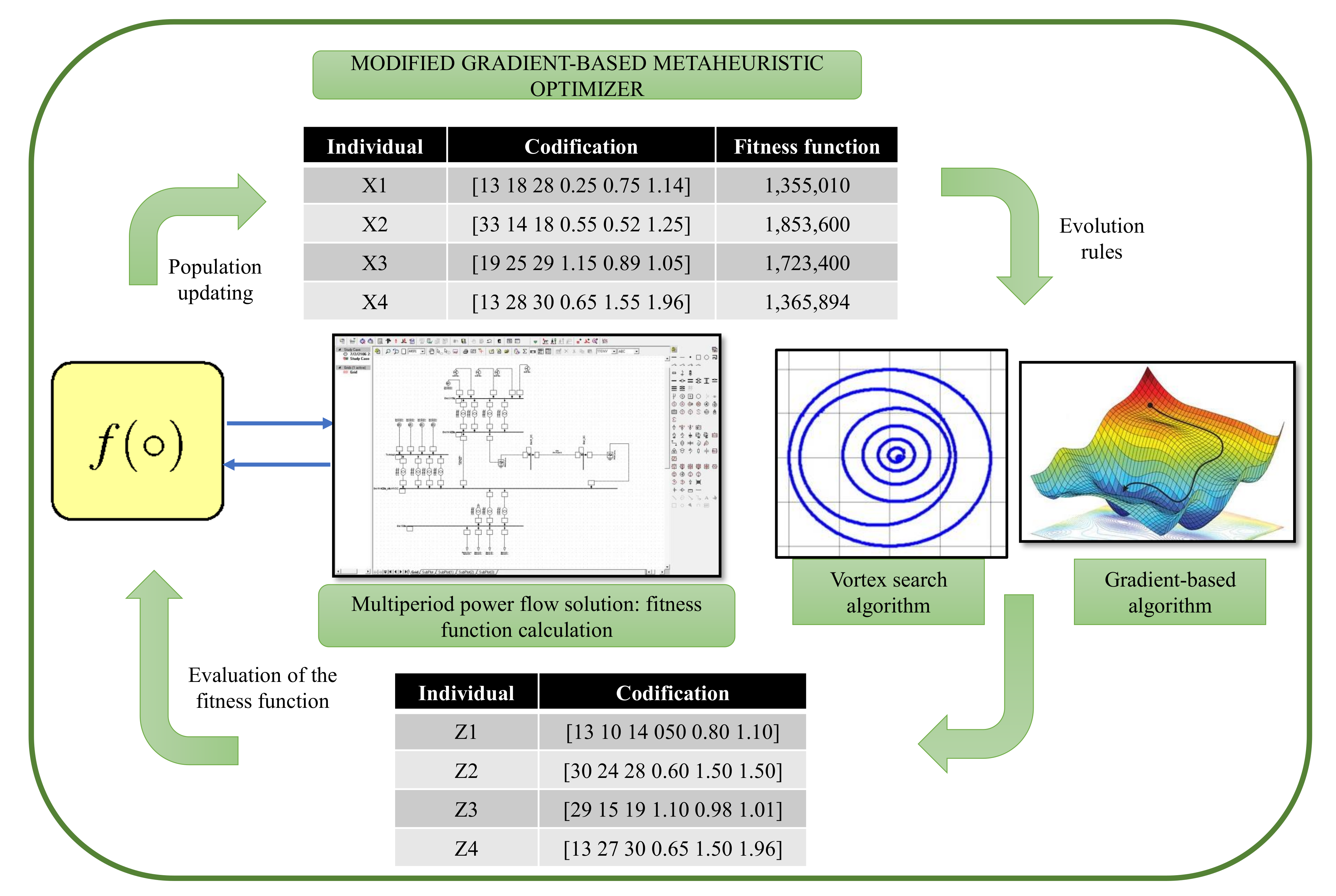
3. Master–Slave Optimization Proposal

To deal with the MINLP structure of the optimization model (1)–(11), Reference [23] proposed the application of the gradient-based metaheuristic optimizer (GbMO) in a master–slave approach combined with the classical successive approximation power flow method. In Ref. [18], the master stage is entrusted with determining the optimal locations and sizes of the PV generation units using a discrete–continuous codification. The codification that represents the studied problem is presented in Equation (12).

$$\begin{array}{c}\hfill Z_i^t=\left[2,k,\cdots ,10|0.2537,0.7898,\cdots ,1.1299\right],\end{array}$$

(12)

where $Z_i^t$ represents the solution of individual i at iteration t. Note that the first $N_{pv}^{ava}$ position of the solution vector in (12) corresponds to the integer number regarding the location of the PV generation units (note that k is an arbitrary node between two and n, n being the size of the set $\mathcal{N}$), while from the position $N_{pv}^{ava}+1$ to $2N_{pv}^{ava}$, there are continuous numbers regarding the optimal placement and sizing of the PV generators. The main advantage of the codification in (12) is that the locations and the sizes of the PV generators are solved using a unique codification [11], which implies that if the vector $Z_i^t$ is completely feasible, then the MINLP model (1)–(11) is reduced to a simple nonlinear programming model where the challenge is the power balance Equations (4) and (5), respectively. The details of the master and slave stages are discussed below.

To illustrate the general implementation of the proposed MGbMO with the inclusion of the vortex search algorithm to improve the exploration and exploitation stages, the general algorithmic structure is shown in Figure 1.

Note that the main characteristics of the proposed optimization methodology are:

✓

Random generation of the initial population at the beginning of the iteration process of the algorithm, with feasibility maintained during all the exploration and exploitation steps on the solution space during all the iterations;

✓

Association of the improvement of the exploration and exploitation stages with the possibility of working with the gradient-based evolution rule or with the application of the vortex search evolution strategy;

✓

Responsibility of the multiperiod power flow solution to calculate the fitness function value, which will guide the exploration and exploitation stages with the proposed MGbMO.

3.1. Master Stage: Gradient-Based Metaheuristic Optimizer

The GbMO is an optimization technique that can deal with complex nonlinear non-convex optimization problems in engineering, developed recently by Ahmadianfar [21]. This optimization method is based on the classical numerical method based on the gradient descendant algorithm to solve unconstrained continuous optimization problems. Here, an easy derivation of the GbMO is presented to solve combinatorial optimization problems. In the case of minimizing an objective function, the gradient method defines the evolution rule presented in Equation (13).

$$\begin{array}{c}\hfill Z_i^{t+1}=Z_i^t-{\alpha }_i^t\nabla f\left(Z_j^t\right),\end{array}$$

(13)

where ${\alpha }_i^t$ is the adaptive step of the gradient search algorithm for the ith in iteration t; $\nabla f\left(Z_i^t\right)$ represents the gradient of the function f evaluated in the current individual $Z_i^t$.

To obtain the gradient of the objective function, the Taylor series expansion is applied to this function [24], which produces the following relation:

$$\begin{array}{c}\hfill f\left(Z_{i+1}^t\right)-f\left(Z_i^t\right)=\left(Z_{i+1}^t-Z_i^t\right)\nabla f\left(Z_i^t\right).\end{array}$$

(14)

Note that to evaluate Equation (14), it is necessary to know the value of the objective function, i.e., $f\left(Z_{i+1}^t\right)$ and $f\left(Z_i^t\right)$, which implies that at this point, the usage of the slave stage is required, which will be described further ahead in this document.

On the other hand, the difference between the current solutions $Z_i^t$ and $Z_{i-1}^t$ can be defined as a parameter, ${\beta }_i^t$, multiplied by the difference of the current solution and the next step, $Z_{i+1}^t$:

$$\begin{array}{c}\hfill Z_i^t-Z_{i-1}^t={\beta }_i^t\left(Z_{i+1}^t-Z_i^t\right).\end{array}$$

(15)

Now, if we combine Equations (13)–(15), the following evolution is obtained:

$$\begin{array}{c}\hfill Z_i^{t+1}=Z_i^t-{\beta }_i^t\frac{{\alpha }_i^t}{∥Z_i^t-Z_{i-1}^t∥}\left(f\left(Z_{i+1}^t\right)-f\left(Z_j^t\right)\right),\end{array}$$

(16)

where $∥z∥$ represents the $l_2$-norm of the vector z.

Note that the exploration qualities of the evolution rule (16) are local since no information regarding the best current solution ($Z_{\mathrm{best}}^t$) is contained in it; for this reason and based on the recommendations in [25], we propose the following adaptive evolution rule:

$$\begin{array}{c}\hfill Z_i^{t+1}=Z_i^t-{\beta }_i^t\frac{{\alpha }_i^t}{∥Z_i^t-Z_{i-1}^t∥}\left(f\left(Z_{i+1}^t\right)-f\left(Z_j^t\right)\right)+{\gamma }_i^t\left(Z_{\mathrm{best}}^t-Z_i^t\right),\end{array}$$

(17)

where:

✓

The ${\beta }_i^t$-coefficient is selected as a binary vector filled with random zero and one values;

✓

The ${\alpha }_i^t$ vector is selected as the solution individual $Z_{i-1}^t$, which is located one position before the current solution $Z_i^t$;

✓

The ${\gamma }_i^t$ vector takes random values between zero and one that weight the effect of the best current solution, i.e., $Z_{\mathrm{best}}^t$, in the movement of the current solution $Z_i^t$.

An important reason to maintain feasibility in the solution space is that for each individual $Z_i^{t+1}$, it is mandatory to revise each component of it to ensure that it is between its lower and upper bounds [26].

3.1.1. Exploration and Exploitation Improvement

To improve the exploration and exploitation characteristics of the general evolution rule (17), this study proposes a modification of the GbMO using the evolution strategy used by the vortex search algorithm (VSA) proposed in [27]. The VSA explores and exploits the solution space through the usage of non-concentric hyper-ellipses generated with a Gaussian distribution, which are generated around the center of the solution space at the current iteration t. This center is named ${\mu }_t$, and in the case of the modified GbMO (MGbMO), the best current solution in the iteration t is selected as the center of the solution space, i.e., ${\mu }_t=Z_{\mathrm{best}}^t$. The generation of the best current solutions around ${\mu }_t$ is made with the following Gaussian distribution:

$$\begin{array}{cc}\hfill Zt+1& =p\left(z\right|{\mu }_t,\Sigma )=\hfill \\ \hfill & =\frac{1}{\sqrt{{\left(2\pi \right)}^{2N_{pv}^{ava}}|\Sigma |)}}exp\left\{-\frac{1}{2}{(\zeta -{\mu }_t)}^T{\Sigma }^{-1}(z-{\mu }_t)\right\},\hfill \end{array}$$

(18)

where $\zeta$ corresponds to a vector with random variables between zero and one; $\Sigma$ is the co-variance matrix. It is important to highlight that in $\Sigma$, the diagonal elements are defined with equal values and the non-diagonal elements with zero values. Then, the Gaussian distribution will generate hyper-ellipses around the center of the solution space [28]. Considering the aforementioned characteristics of the co-variance matrix, this can be easily defined as:

$$\Sigma ={\sigma }_0\mathbf{I},$$

(19)

where ${\sigma }_0$ is defined as the standard deviation of the Gaussian distribution and $\mathbf{I}$ is defined as an identity matrix with appropriate size. In the case of the initial exploration and exploitation of the solution space, the initial standard deviation is calculated as defined in Equation (20).

$${\sigma }_0=\frac{max\left\{x^{max}\right\}-min\left\{x^{min}\right\}}{2},$$

(20)

where ${\sigma }_0$ is also known as the maximum radius of the solution space at the beginning of the iteration process (i.e., $r_0$), which will decrease as the number of iterations increases [27]. Note that $x^{max}$ and $x^{min}$ are the vectors that contains all the upper and lower bounds admissible for the decision variables in the vector $Z_i^t$ defined in (12). In this research, we propose that the decreasing rate applied for the radius $r_t$ be a linear function of the number of iterations, i.e.,

$$\begin{array}{c}\hfill r_t=1-\frac{t}{t_{max}}.\end{array}$$

(21)

As in the case of the GbMO, once all the individuals in the population $Z^{t+1}$ have been created, each one of them must be carefully revised to ensure that the decision variables are contained within their lower and upper bounds. Additionally, the first $N_{ava}^{pv}$ positions are rounded to the nearest integer to ensure the discrete nature of the codification vector presented in (12), which is associated with the nodes where the PV generation units will be installed.

3.1.2. Proposed MGbMO

Algorithm 1 is presented to illustrate the general implementation of the MGbMO solution methodology to deal with the problem of optimal placement and sizing of PV generation units in medium-voltage distribution grids.

3.2. Slave Stage: Successive Approximation Power Flow

The main complication in optimizations problems of distribution systems is when the whole grid model is considered, i.e., the power balance constraints in the solution of these equations, since these are highly nonlinear and non-convex, which implies that numerical methods are required in their solution [23]. Even if the solution of the power flow problem is fundamental for the implementation of metaheuristics, there now exist multitudes of solution methods to deal with this problem, as is the case of the successive approximation power flow method [23]. Nevertheless, the real advantage of using metaheuristics to solve MINLP models corresponds to the possibility of decoupling the binary problem (the location of PV generation units) from the continuous problem (power flow solution). In the slave stage, it is assumed that the problem of the placement and sizing of the PV generation units is solved with the codification in (12), which implies that to determine the objective function value (1), it is necessary to know the power flow solution. Here, the recursive power flow formula reported in [23] was adopted, which can work with radial and meshed distribution grids.

$$\begin{array}{c}\hfill {\mathbb{V}}_{d,h}^{m+1}={\mathbb{Y}}_{dd}^{-1}\left[{\mathbf{diag}}^{-1}\left({\mathbb{V}}_{d,h}^m\right)\left({\mathbb{S}}_{pv,h}^{★}-{\mathbb{S}}_{d,h}^{★}\right)-{\mathbb{Y}}_{ds}{\mathbb{V}}_{s,h}\right],\end{array}$$

(22)

where m is the iterative counter; ${\mathbb{V}}_d$ is the vector that contains all the voltage variables in the complex domain for all the demand nodes at each period of time h; ${\mathbb{S}}_{pv,h}$ is the complex vector that contains all the power generations in the PV generation units at each period of time h (note that this vector is provided by the master stage as an input for the power flow problem); ${\mathbb{S}}_{d,h}$ is the complex demand vector with the active and reactive power consumption in the demand nodes at each period of time; ${\mathbb{V}}_{s,h}$ is the complex voltage output at the substation bus; ${\mathbb{Y}}_{dd}$ is a complex square matrix that contains all the admittances among demand nodes; ${\mathbb{Y}}_{ds}$ is a rectangular complex matrix that contains the admittances between the demand and the substation buses. Note that $\mathbf{diag}\left(z\right)$ and $z^{★}$ are a matrix with all the elements of z at its diagonal and the conjugate operator of the complex vector z, respectively.

Algorithm 1. Proposed optimization methodology based on the modification of the GbMO

The main advantage of using the recursive power flow Formula (22) is that its convergence is ensured with the application of the Banach fixed-point theorem, as demonstrated in [22]. Here, to define that the power flow problem is solved with the help of (22), the difference of the voltage magnitudes between two consecutive iterations was used as follows:

$$\begin{array}{c}\hfill \underset{h}{max}\left\{\left|\right|{\mathbb{V}}_{d,h}^{m+1}|-|{\mathbb{V}}_{d,h}^m\left|\right|\right\}\le \epsilon ,\end{array}$$

(23)

where $\epsilon$ is the tolerance value, which is assigned as $1\times {10}^{-10}$, as recommended in [23].

Once the power flow problem has been solved, the active power generation in the slack bus is calculated with the following formula:

$$\begin{array}{c}\hfill p_{i,h}^{cg}=\mathrm{real}\left\{{\mathbb{S}}_{s,h}\right\}=\mathrm{real}\left\{\mathbf{diag}\left({\mathbb{V}}_{s.h}\right)\left({\mathbb{Y}}_{ss}^{★}{\mathbb{V}}_{s,h}^{★}+{\mathbb{Y}}_{sd}^{★}{\mathbb{V}}_{d,h}^{★}\right)\right\},\end{array}$$

(24)

Note that with the solution of $p_{i,h}^{cg}$ in (14), it is possible to determine the first component of the objective function, i.e., $f_1$, while the solution vector provided by the master stage is where the sizes of the PV sources are assigned; then, the second component of the objective function, i.e., $f_2$, is calculated. However, as is well known in metaheuristic optimizers, the exploration and exploitation of the solution space are performed through the application of an adapted objective function named the fitness function ($F_f$) [29]. The proposed fitness function contains two penalty factors regarding the voltage regulation constraint and an additional penalty factor regarding the positive definiteness of the active power generation in the slack source; this is defined by Equation (25).

$$\begin{array}{c}\hfill F_f=A_{\mathrm{cost}}+\left[\begin{array}{c}{\theta }_1\underset{h}{max}\left\{|{\mathbb{V}}_{d,h}|-v_d^{max},0\right\}+{\theta }_2\underset{h}{max}\left\{|v_d^{min}-\left|{\mathbb{V}}_{d,h}\right|,0\right\}-{\theta }_3\underset{h}{min}\left\{p_{i,h}^{cg},0\right\}\end{array}\right],\end{array}$$

(25)

where ${\theta }_1$, ${\theta }_2$, and ${\theta }_3$ are positive penalty factors that are activated in the case of the violation of the voltage regulation and active power generation bounds in the substation bus (these penalty factors were set as $100\times {10}^3$).

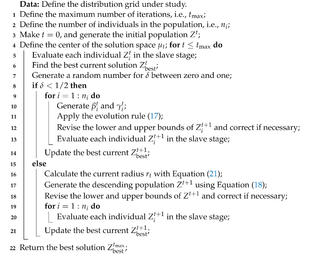
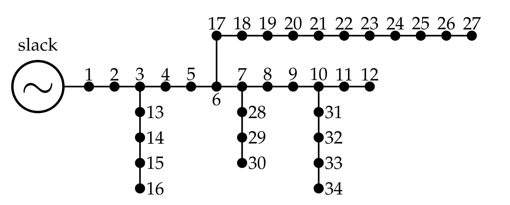
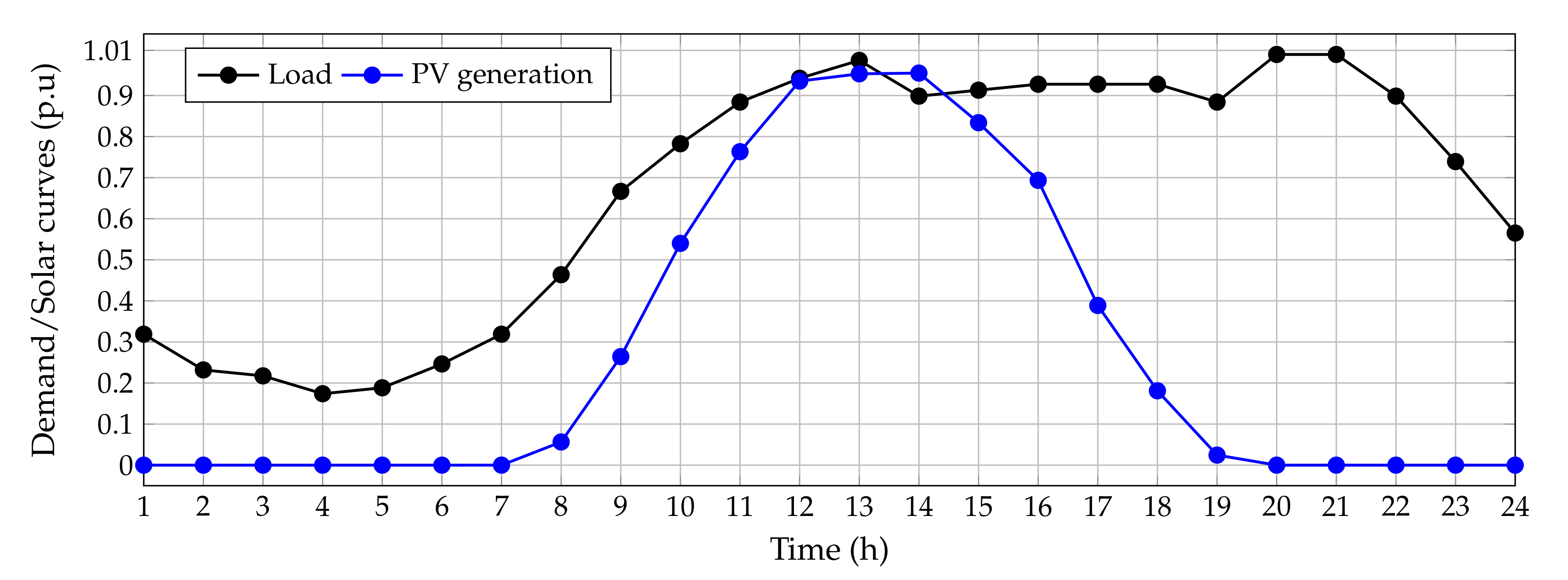
4. Test Feeder Information

The assessment of the proposed MGbMO to place and size PV generation units in medium-voltage distribution networks was conducted in the IEEE 34-bus system, depicted in Figure 2. This is a medium-voltage network operated with 11 kV in the substation bus, with a total of $4636.50+j2873.50$ kVA power consumption in the peak load condition and a total of $221.75+j65.12$ kVA active and reactive power losses [30].

The electrical information about demands in all the nodes and reactances and resistances in branches is listed in

Table 2. Load and line parameters for the IEEE 34-bus system.

k	m	Rkm (Ω)	xkm (Ω)	Pk (kW)	Qk (kW)
1	2	0.1170	0.0480	230	142.5
2	3	0.1073	0.0440	0	0
3	4	0.1645	0.0457	230	142.5
4	5	0.1495	0.0415	230	142.5
5	6	0.1495	0.0415	0	0
6	7	0.3144	0.0540	0	0
7	8	0.2096	0.0360	230	142.5
8	9	0.3144	0.0540	230	142.5
9	10	0.2096	0.0360	0	0
10	11	0.1310	0.0225	230	142.5
11	12	0.1048	0.0180	137	84
3	13	0.1572	0.0270	72	45
13	14	0.2096	0.0360	72	45
14	15	0.1048	0.0180	72	45
15	16	0.0524	0.0090	13.5	7.5
6	17	0.1794	0.0498	230	142.5
17	18	0.1645	0.0457	230	142.5
18	19	0.2079	0.0473	230	142.5
19	20	0.1890	0.0430	230	142.5
20	21	0.1890	0.0430	230	142.5
21	22	0.2620	0.0450	230	142.5
22	23	0.2620	0.0450	230	142.5
23	24	0.3144	0.0540	230	142.5
24	25	0.2096	0.0360	230	142.5
25	26	0.1310	0.0225	230	142.5
26	27	0.1048	0.0180	137	85
7	28	0.1572	0.0270	75	48
28	29	0.1572	0.0270	75	48
29	30	0.1572	0.0270	75	48
10	31	0.1572	0.0270	57	34.5
31	32	0.2096	0.0360	57	34.5
32	33	0.1572	0.0270	57	34.5
33	34	0.1048	0.0180	57	34.5

[30].

To determine the value of the objective function regarding the energy purchasing costs and the PV installation and maintenance costs, the information presented in

Table 3. Parametrization of the fitness function evaluation.

Param.	Value	Unit	Param.	Value	Unit
$C_{\mathrm{kWh}}$	0.1390	USD/kWh	T	365	days
$t_a$	10	%	$t_e$	2	%
$N_t$	20	years	$\Delta h$	1	h
$C_{\mathrm{PV}}$	1036.49	USD/kWp	$C_{O\&M}$	0.0019	USD/kWh
$p_i^{pv,max}$	2400	kW	$p_i^{pv,min}$	0	kW
$N_{pv}^{ava}$	3	—	$\Delta V$	±10	%
${\alpha }_1$	$100\times {10}^3$	USD/V	${\alpha }_2$	$100\times {10}^3$	USD/V
${\alpha }_3$	$100\times {10}^3$	USD/W	—	—	—

was used [11].

Finally, to emulate the expected daily generation behavior with PV sources and the demand consumption, typical curves obtained in the metropolitan area of the Colombian city of Medellín were employed. This information was provided by the authors of [31].

It is worth emphasizing that Colombia is a country located in the equatorial region; the weather throughout the year varies somewhat, but not the seasons, which implies that the demand and PV curves in Figure 3 can be considered as the average curves for all the days in an ordinary year.

5. Numerical Validation

To demonstrate the effectiveness of the proposed MGbMO to solve the studied problem, this proposal was compared with the current literature algorithms from the metaheuristic optimizers family. These algorithms are: the Chu and Beasley genetic algorithm (CBGA) [11]; the Newton metaheuristic algorithm (NMA) [18]; the original GbMO [21]; the BONMIN solver in the general algebraic modeling system (GAMS) software [17]. Note that the implementation of the metaheuristic optimizers was performed with MATLAB 2021b using the researchers’ own scripts on a PC with an AMD Ryzen 7 3700 $2.3$-GHz processor and 16.0 GB RAM, running on a 64 bit version of Microsoft Windows 10 Single language. In addition, to evaluate all the metaheuristic optimizers, a population size of 10 individuals, 1000 iterations, and 100 repetitions of each algorithm were considered.

The best optimal solution for the proposed MGbMO and the comparative methodologies are reported in

Table 4. Comparative results in the IEEE 34-bus grid when compared with the proposed MGbMO and the literature reports.

Method	Site (Node) Size (kW)	Acost (USD/Year)	Proc. Time (s)
Bench. case	—	4,588,283.80	—
BONMIN	{26(2400), 27(747.45), 34(1336.00)}	3,355,261.86	5.475
DCCBGA	{11(1055.54), 23(1347.95), 25(2057.09)}	3,354,711.16	5.977
NMA	{10(994.25), 23(1409.42), 24(2056.85)}	3,354,676.16	21.285
GbMO	{11(1554.01), 21(1337.90) 26(1541.03)}	3,355,105.86	24.126
MGbMO	{11(1064.55), 23(2050.01), 25(1340.94)}	3,354,495.20	21.867

. Numerical results in this table show that:

✓

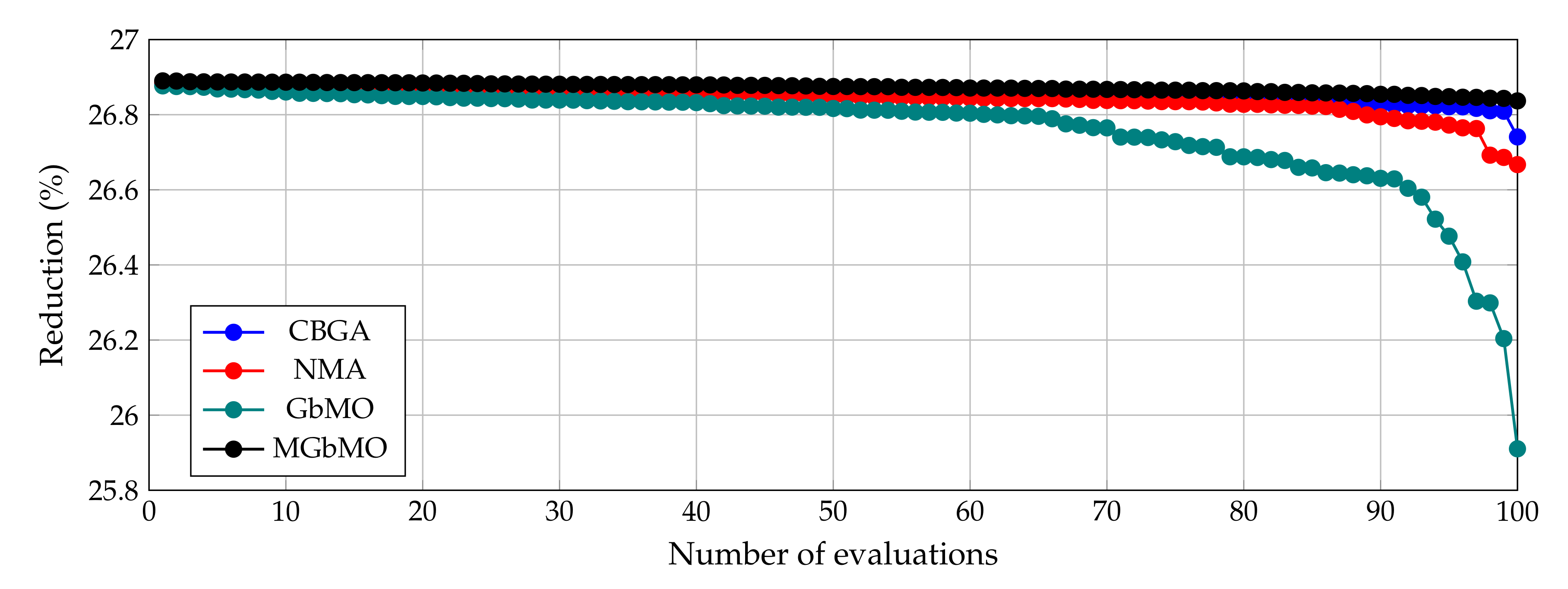
The best current solution for the IEEE 34-bus system was found by the proposed MGbMO with an annual operative cost value of USD 3,354,495.20 per year. This solution was obtained by locating the PV units at Nodes 11, 23, and 25, with a total nominal generation capacity of $4455.50$ kW. In addition, this solution allows for the reduction of the grid’s operating costs by about 26.89%, about USD 1,233,788.60 per year of operation, with respect to the benchmark case;

✓

The second-best solution for the IEEE 34-bus system was found by the NMA with an annual reduction of USD 1,233,607.64, implying that the proposed MGbMO allows an additional reduction of about USD $180.96$ per year of operation;

✓

The original GbMO solves the studied problem by reaching an objective function of about USD 3,355,105.86 per year, which is better than the solution obtained by the GAMS optimization solver with the BONMIN solver; however, the proposed improvement of this algorithm with the vortex search exploration and exploitation characteristics showed that an additional USD $610.96$ per year of operation can be recovered with the proposed method;

✓

Regarding processing times, it is important to mention that all algorithms took less than 25 s to solve the studied problem. This is an excellent time for any master–slave optimization approach that solves planning problems since it permits hundreds of evaluations to be conducted prior to the final decision regarding the physical implementation of the optimal solution.

To illustrate the general performance of the metaheuristic optimizers after each one of the 100 evaluations, the general efficiency of each of the algorithms with respect to the benchmark case is plotted in Figure 4.

The results in Figure 4 show that: (i) the proposed MGbMO is the only solution methodology that maintains its solutions during the 100 consecutive evaluations, with improvements higher than 26.84% with respect to the benchmark case; this implies that it ensures cost reductions higher than USD 1,231,342.42 per year in all the solution cases; (ii) in terms of algorithm stability, the second-best performance was reached by the CBGA followed by the NMA, since this ensured improvements of the objective function higher than 26.74% and 26.67% with respect to the benchmark case; (iii) the original GbMO presented higher oscillations during the solution process, which are attributable to the presence of a difference between two values of the objective function in its evolution Formula (12); however, these oscillations were minimized with the introduction of the adaptive exploration and exploitation stages based on the hyper-ellipses with a variable radius.

To ensure that all the voltages in all the nodes of the network were within their upper and lower bounds throughout the day, the maximum and minimum voltage magnitudes obtained in the IEEE 34-bus system when the solution of the proposed MGbMO was implemented are plotted in Figure 5.

The most important result in Figure 5 is that all the voltages in the distribution network were maintained between their assigned voltage regulation bounds during the daily operation, i.e., ±10%. The worst voltage case occurred for Hours 20 and 21, where the active power injection from the PV units was null and the demand was under its peak operating condition. The minimum voltage coincided with the benchmark case, i.e., $0.9417$ pu. Nonetheless, for the period of time where the PV generation was maximum, i.e., Hour 14, the voltage in some nodes exceeded the slack voltage with a magnitude of $1.0183$ pu, which was the result of the low demand and high PV power injection.

Finally, to ensure that the generation in the slack node fulfilled the positive definite condition, the slack power generations for the benchmark case and the proposed MGbMO solution are compared in Figure 6.

As expected for the benchmark case, the behavior of the active power generation in terminals of the substation followed the demand curve in Figure 3. Nevertheless, when the PV generation units provided by the proposed MGbMO were installed in the distribution network, the generation requirements in the slack source decreased considerably, zero in the case of the maximum PV generation, i.e., Hour 14, which produced the typical duck curve. The result shown in Figure 6 confirms that the MGbMO generation in the slack source was always positive or zero, which was a condition imposed by the fitness function in (25), since this proposal did not consider the possibility of selling energy to the transmission system.

Extension to Meshed Grids

In order to validate the effectiveness of the proposed MGbMO to solve the problem of the optimal placement and sizing of PV generation units in distribution networks with meshed operative conditions,

Table 5. Additional lines for the meshed configuration if the IEEE 34-bus system.

Node k	Node m	Rkm (Ω)	xkm (Ω)
12	25	0.1310	0.0225
16	30	0.2096	0.0360
30	34	0.1886	0.0310

presents the application of this optimization method to a modification of the IEEE 34-bus system that includes three additional lines with the information as listed.

The first five results obtained after 100 consecutive evaluations of our proposed MGbMO in this meshed configuration are reported in

Table 6. Best five solutions reached with the MGbMO in the meshed configuration of the IEEE 34-bus grid.

Solution Number	Site (Node)—Size (kW)	Acost (USD/Year)
Bench. case	—	4,532,947.02
Solution 1	{21(1727.43), 23(467.41), 25(1920.32)}	3,327,455.92
Solution 2	{20(1249.11), 23(1386.91), 26(1779.56)}	3,327,474.92
Solution 3	{20(1229.27), 23(896.28), 25(2287.21)}	3,327,481.21
Solution 4	{21(787.26), 23(1584.50) 25(2046.15)}	3,327,482.45
Solution 5	21(1129.60), 23(1591.20), 25(1696.55)}	3,327,486.36

.

The numerical results in Table 6 show that:

✓

The difference between benchmark cases was about USD $\mathrm{55,336.78}$ per year when the radial (see Table 4) and meshed configurations were compared, and the difference between both optimal solutions was about USD $\mathrm{27,039.28}$ per year. These results confirm that the meshed configuration allows the amount of power losses in the whole distribution network to be reduced, which is represented by a reduction of the total energy generation requirements in the slack source when compared with the radial configuration case;

✓

The maximum benefit in the meshed configuration case was reached with the first solution, with a reduction of 26.59% with respect to the benchmark case, i.e., USD $\mathrm{1,205,491.10}$ per year. In addition, the difference between the first five solutions was less than USD $30.44$ per year of operation, which confirms the stability of the proposed MGbMO to deal with the problem of the optimal placement and sizing of PV generation sources in distribution grids;

✓

In all the first five solutions, the proposed MGbMO found Nodes 23 and 25 as the optimal locations for the PV sources and Nodes 20 and 21 as varying among these solutions. The total peak power injection in the first solution was about USD $4115.16$ kW, while the fifth solution had a value of USD $4417.36$ kW, which is a difference of less than 2 kW. These results confirm that the proposed MGbMO reaches solutions that are closer to one another and are constrained to a small radius hyper-sphere around the average solution (i.e., USD $\mathrm{3,327,970.82}$ per year).

Regarding processing times, it is important to mention that after the 100 consecutive evaluations, the MGbMO took about 19.950 s to solve the studied problem in the meshed configuration, which is about $1.917$ s faster than the radial configuration. This behavior was expected since for distribution networks, the total number of iterations required by the power flow solution is reduced when a meshed configuration is introduced [23].

6. Conclusions and Future Works

The problem of the optimal placement and sizing of PV generation units in medium-voltage distribution grids was addressed in this research through the application of the gradient-based metaheuristic optimizer and an improvement based on the vortex search algorithm for radial and meshed distribution grid configurations. The main limitation of the proposed approach is associated with the non-consideration of battery energy storage systems in the mathematical formulation since these devices will help with additional improvements in the final operative costs of the distribution network; despite this, the numerical results in the IEEE 34-bus system showed that:

i.

The proposed MGbMO reached the best current solution for this system in the current literature with a reduction about 26.89% of the total annual operative costs with respect to the benchmark case in the radial configuration and 26.59% in the meshed configuration. In the case of the radial configuration, the achieved result corresponded to an improvement of about USD $180.96$ per year with respect to the best current solution reported by the NMA in the current literature;

ii.

The improvement in the exploration and exploitation characteristics of the GbMO by using the hyper-ellipses with a variable radius around the best current solution $Z_{\mathrm{best}}^t$ allowed the proposed MGbMO to have the most stable behavior during all 100 iterations, with reductions higher than 26.84% with respect to the benchmark case in the radial configuration scenario, which was only followed by the CBGA with improvements higher than 26.74%. In the case of the meshed configuration, the proposed MGbMO showed an average reduction of USD 26.58% with respect to the benchmark case, i.e., a difference of 0.01% with respect to the optimal solution;

iii.

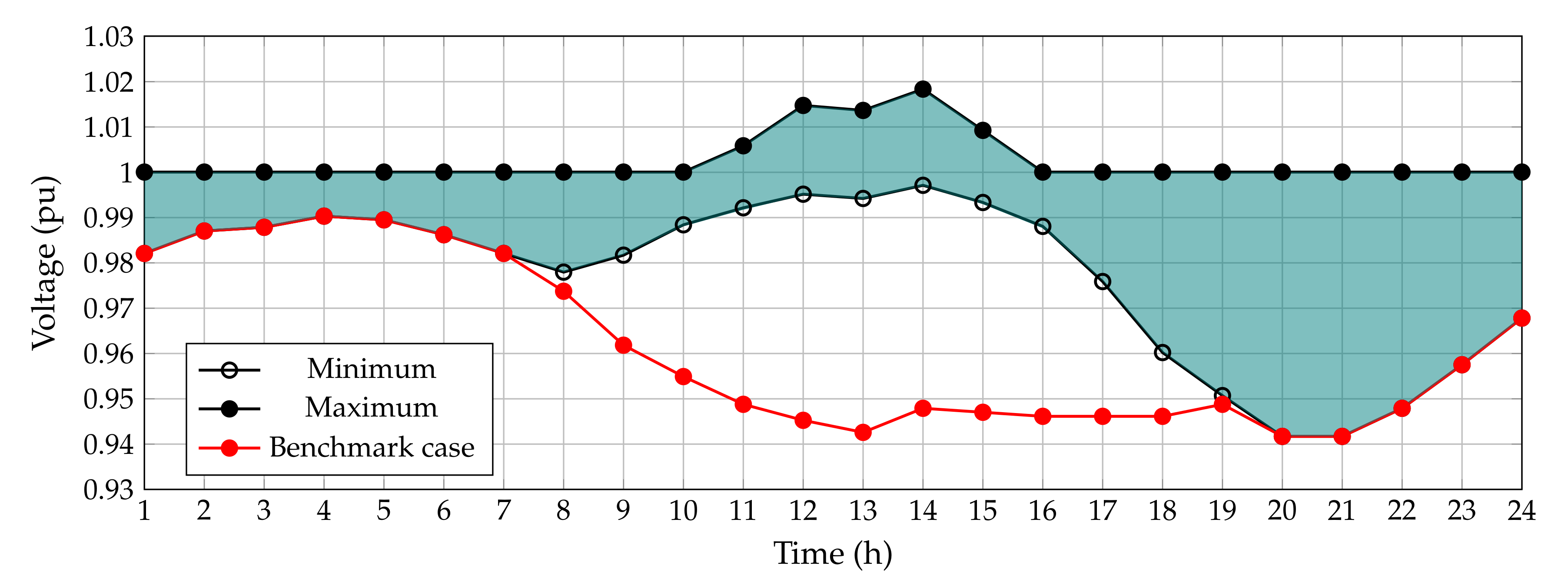
The voltage profiles’ behavior throughout the day in the radial simulations scenario showed that for all the nodes of the system, these were between ±10%, the worst case being when the PV generation was at the minimum (Hour 20 or 21) with a magnitude of $0.9417$ pu and when the PV generation was at the maximum (Hour 14), the voltages in some nodes exceeding the slack voltage with a magnitude of 1.0183 pu;

iv.

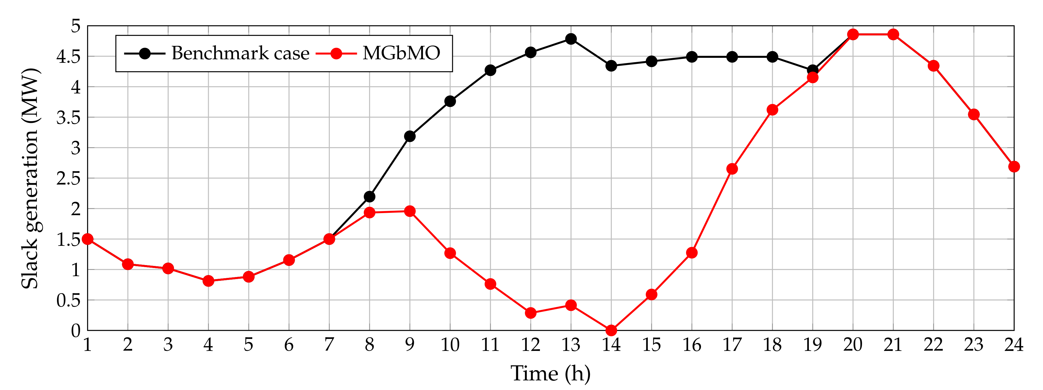
In the case of the slack power generation, the benchmark case showed that this variable followed the demand generation curve; however, when the PV generation was installed, the well-know duck curve was obtained in the slack source (in the radial configuration), which had a zero value when the PV generation was at the maximum, demonstrating that all the model constraints were satisfied by the studied solution method. This behavior was also confirmed in the meshed configuration.

For future studies, it will be possible to develop the following research:

i.

Consider the possibility of variable generation output in the PV sources throughout the day (between zero and the nominal generation curve), which will help to find additional objective function improvements;

ii.

Study the simultaneous location of distribution static compensators and PV generation units in distribution networks for annual operative costs’ minimization;

iii.

Propose a mixed-integer conic formulation to solve the MINLP model studied in this research in order to ensure the global optimum finding without referring to statistical validations;

iv.

Apply the Harris hawks optimization algorithm and the water cycle algorithm to solve the problem of the optimal placement and sizing of renewable energy sources in distribution grids and compare their efficiency and robustness with the MGbMO proposed in this research.

References

1. Lavorato, M.; Rider, M.J.; Garcia, A.V.; Romero, R. A Constructive Heuristic Algorithm for Distribution System Planning. IEEE Trans. Power Syst. 2010, 25, 1734–1742. [Google Scholar] [CrossRef]
2. Girbau-Llistuella, F.; Díaz-González, F.; Sumper, A.; Gallart-Fernández, R.; Heredero-Peris, D. Smart Grid Architecture for Rural Distribution Networks: Application to a Spanish Pilot Network. Energies 2018, 11, 844. [Google Scholar] [CrossRef] [Green Version]
3. Helmi, A.M.; Carli, R.; Dotoli, M.; Ramadan, H.S. Efficient and Sustainable Reconfiguration of Distribution Networks via Metaheuristic Optimization. IEEE Trans. Autom. Sci. Eng. 2022, 19, 82–98. [Google Scholar] [CrossRef]
4. Nahman, J.; Peric, D. Optimal Planning of Radial Distribution Networks by Simulated Annealing Technique. IEEE Trans. Power Syst. 2008, 23, 790–795. [Google Scholar] [CrossRef]
5. Lavorato, M.; Franco, J.F.; Rider, M.J.; Romero, R. Imposing Radiality Constraints in Distribution System Optimization Problems. IEEE Trans. Power Syst. 2012, 27, 172–180. [Google Scholar] [CrossRef]
6. Paz-Rodríguez, A.; Castro-Ordoñez, J.F.; Montoya, O.D.; Giral-Ramírez, D.A. Optimal Integration of Photovoltaic Sources in Distribution Networks for Daily Energy Losses Minimization Using the Vortex Search Algorithm. Appl. Sci. 2021, 11, 4418. [Google Scholar] [CrossRef]
7. Tolmasquim, M.T.; Linhares-Pires, J.C.; Rosa, L.P. New Strategies for Power Companies in Brazil. In European Energy Industry Business Strategies; Elsevier: Amsterdam, The Netherlands, 2001; pp. 337–374. [Google Scholar] [CrossRef]
8. Jerez, S.; Tobin, I.; Vautard, R.; Montávez, J.P.; López-Romero, J.M.; Thais, F.; Bartok, B.; Christensen, O.B.; Colette, A.; Déqué, M.; et al. The impact of climate change on photovoltaic power generation in Europe. Nat. Commun. 2015, 6, 10014. [Google Scholar] [CrossRef] [Green Version]
9. Steffen, B.; Beuse, M.; Tautorat, P.; Schmidt, T.S. Experience Curves for Operations and Maintenance Costs of Renewable Energy Technologies. Joule 2020, 4, 359–375. [Google Scholar] [CrossRef]
10. López, A.R.; Krumm, A.; Schattenhofer, L.; Burandt, T.; Montoya, F.C.; Oberländer, N.; Oei, P.Y. Solar PV generation in Colombia—A qualitative and quantitative approach to analyze the potential of solar energy market. Renew. Energy 2020, 148, 1266–1279. [Google Scholar] [CrossRef]
11. Montoya, O.D.; Grisales-Noreña, L.F.; Perea-Moreno, A.J. Optimal Investments in PV Sources for Grid-Connected Distribution Networks: An Application of the Discrete–Continuous Genetic Algorithm. Sustainability 2021, 13, 13633. [Google Scholar] [CrossRef]
12. Kaur, S.; Kumbhar, G.; Sharma, J. A MINLP technique for optimal placement of multiple DG units in distribution systems. Int. J. Electr. Power Energy Syst. 2014, 63, 609–617. [Google Scholar] [CrossRef]
13. Muhammad, M.A.; Mokhlis, H.; Naidu, K.; Amin, A.; Franco, J.F.; Othman, M. Distribution Network Planning Enhancement via Network Reconfiguration and DG Integration Using Dataset Approach and Water Cycle Algorithm. J. Mod. Power Syst. Clean Energy 2020, 8, 86–93. [Google Scholar] [CrossRef]
14. Prenc, R.; Skrlec, D.; Komen, V. Optimal PV system placement in a distribution network on the basis of daily power consumption and production fluctuation. In Proceedings of the Eurocon 2013, Zagreb, Croatia, 1–4 July 2013. [Google Scholar] [CrossRef]
15. Hraiz, M.D.; Garcia, J.A.M.; Castaneda, R.J.; Muhsen, H. Optimal PV Size and Location to Reduce Active Power Losses While Achieving Very High Penetration Level with Improvement in Voltage Profile Using Modified Jaya Algorithm. IEEE J. Photovoltaics 2020, 10, 1166–1174. [Google Scholar] [CrossRef]
16. Valencia, A.; Hincapie, R.A.; Gallego, R.A. Optimal location, selection, and operation of battery energy storage systems and renewable distributed generation in medium–low voltage distribution networks. J. Energy Storage 2021, 34, 102158. [Google Scholar] [CrossRef]
17. Soroudi, A. Power System Optimization Modeling in GAMS; Springer International Publishing: Berlin/Heidelberg, Germany, 2017. [Google Scholar] [CrossRef]
18. Montoya, O.D.; Grisales-Noreña, L.F.; Alvarado-Barrios, L.; Arias-Londoño, A.; Álvarez-Arroyo, C. Efficient Reduction in the Annual Investment Costs in AC Distribution Networks via Optimal Integration of Solar PV Sources Using the Newton Metaheuristic Algorithm. Appl. Sci. 2021, 11, 11525. [Google Scholar] [CrossRef]
19. Wang, P.; Wang, W.; Xu, D. Optimal Sizing of Distributed Generations in DC Microgrids with Comprehensive Consideration of System Operation Modes and Operation Targets. IEEE Access 2018, 6, 31129–31140. [Google Scholar] [CrossRef]
20. Chen, X.; Li, Z.; Wan, W.; Zhu, L.; Shao, Z. A master–slave solving method with adaptive model reformulation technique for water network synthesis using MINLP. Sep. Purif. Technol. 2012, 98, 516–530. [Google Scholar] [CrossRef]
21. Ahmadianfar, I.; Bozorg-Haddad, O.; Chu, X. Gradient-based optimizer: A new metaheuristic optimization algorithm. Inf. Sci. 2020, 540, 131–159. [Google Scholar] [CrossRef]
22. Shen, T.; Li, Y.; Xiang, J. A Graph-Based Power Flow Method for Balanced Distribution Systems. Energies 2018, 11, 511. [Google Scholar] [CrossRef] [Green Version]
23. Montoya, O.D.; Gil-González, W. On the numerical analysis based on successive approximations for power flow problems in AC distribution systems. Electr. Power Syst. Res. 2020, 187, 106454. [Google Scholar] [CrossRef]
24. Deb, S.; Abdelminaam, D.S.; Said, M.; Houssein, E.H. Recent Methodology-Based Gradient-Based Optimizer for Economic Load Dispatch Problem. IEEE Access 2021, 9, 44322–44338. [Google Scholar] [CrossRef]
25. Gholizadeh, S.; Danesh, M.; Gheyratmand, C. A new Newton metaheuristic algorithm for discrete performance-based design optimization of steel moment frames. Comput. Struct. 2020, 234, 106250. [Google Scholar] [CrossRef]
26. Randall, M. Feasibility Restoration for Iterative Meta-heuristics Search Algorithms. In Developments in Applied Artificial Intelligence; Springer: Berlin/Heidelberg, Germany, 2002; pp. 168–178. [Google Scholar] [CrossRef] [Green Version]
27. Doğan, B.; Ölmez, T. A new metaheuristic for numerical function optimization: Vortex Search algorithm. Inf. Sci. 2015, 293, 125–145. [Google Scholar] [CrossRef]
28. Gharehchopogh, F.S.; Maleki, I.; Dizaji, Z.A. Chaotic vortex search algorithm: Metaheuristic algorithm for feature selection. Evol. Intell. 2021. [Google Scholar] [CrossRef]
29. Sahin, O.; Akay, B. Comparisons of metaheuristic algorithms and fitness functions on software test data generation. Appl. Soft Comput. 2016, 49, 1202–1214. [Google Scholar] [CrossRef]
30. Tamilselvan, V.; Jayabarathi, T.; Raghunathan, T.; Yang, X.S. Optimal capacitor placement in radial distribution systems using flower pollination algorithm. Alex. Eng. J. 2018, 57, 2775–2786. [Google Scholar] [CrossRef]
31. Grisales-Noreña, L.; Montoya, O.D.; Ramos-Paja, C.A. An energy management system for optimal operation of BSS in DC distributed generation environments based on a parallel PSO algorithm. J. Energy Storage 2020, 29, 101488. [Google Scholar] [CrossRef]
Figure 1. General algorithmic structure of the proposed MGbMO.
Sustainability 14 03318 g001
Figure 2. Electrical configuration of the IEEE 34-bus system.
Sustainability 14 03318 g002
Figure 3. Demand and generation curves typical for Medellín, Colombia.
Sustainability 14 03318 g003
Figure 4. Average performance of the metaheuristic optimizers.
Sustainability 14 03318 g004
Figure 5. Minimum and maximum voltage magnitudes in the IEEE 34-node test feeder when the MGbMO solution was implemented.
Sustainability 14 03318 g005
Figure 6. Generation output in the slack source for the benchmark case and the solution of our proposed MGbMO.
Sustainability 14 03318 g006