
Flood Hazard and Risk Mapping by Applying an Explainable Machine Learning Framework Using Satellite Imagery and GIS Data

 , , , ,
  ,
, 
 ,
,  and
and 
Abstract
:1. Introduction
2. Relevant Literature
3. Materials and Methods
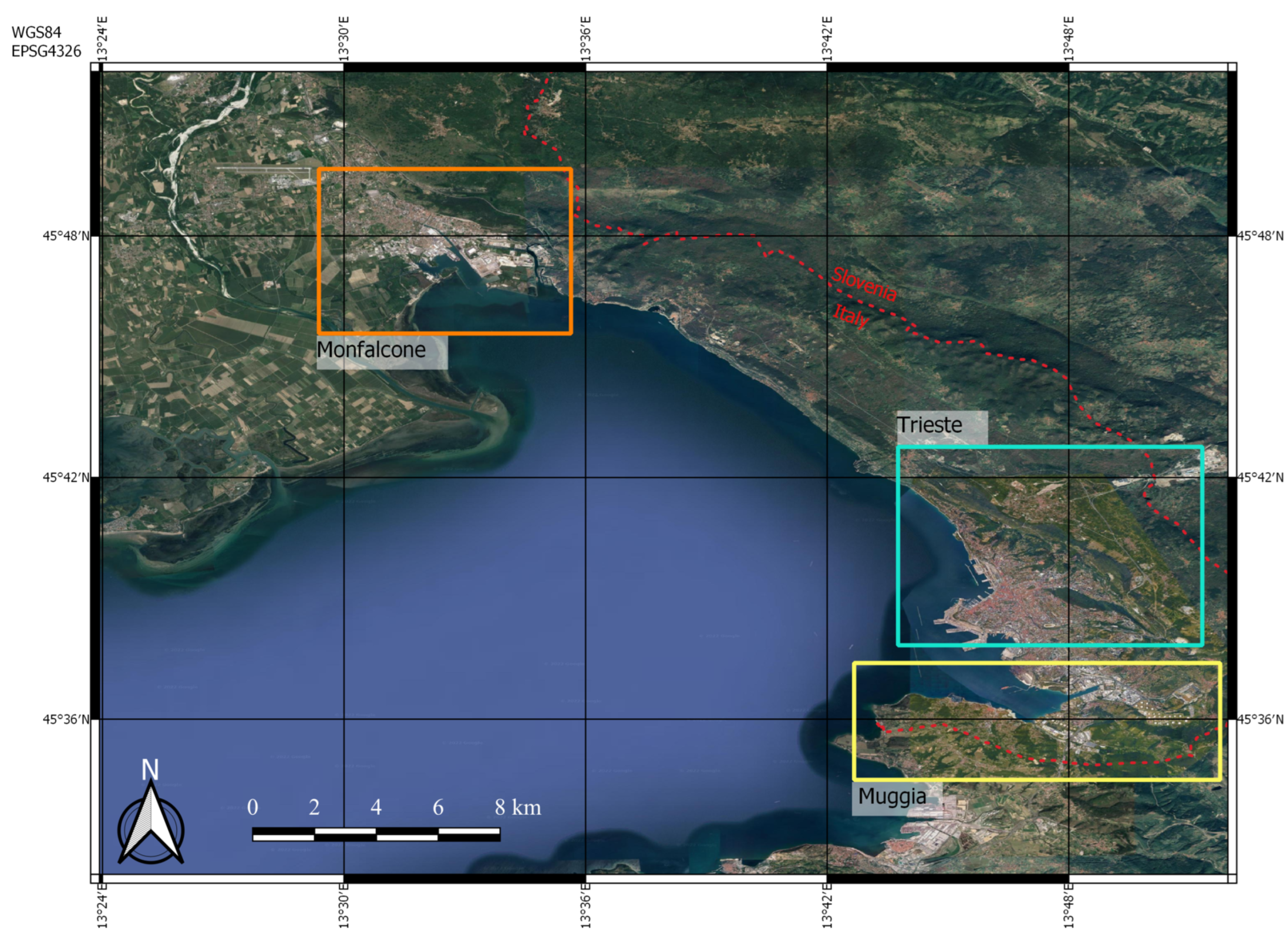
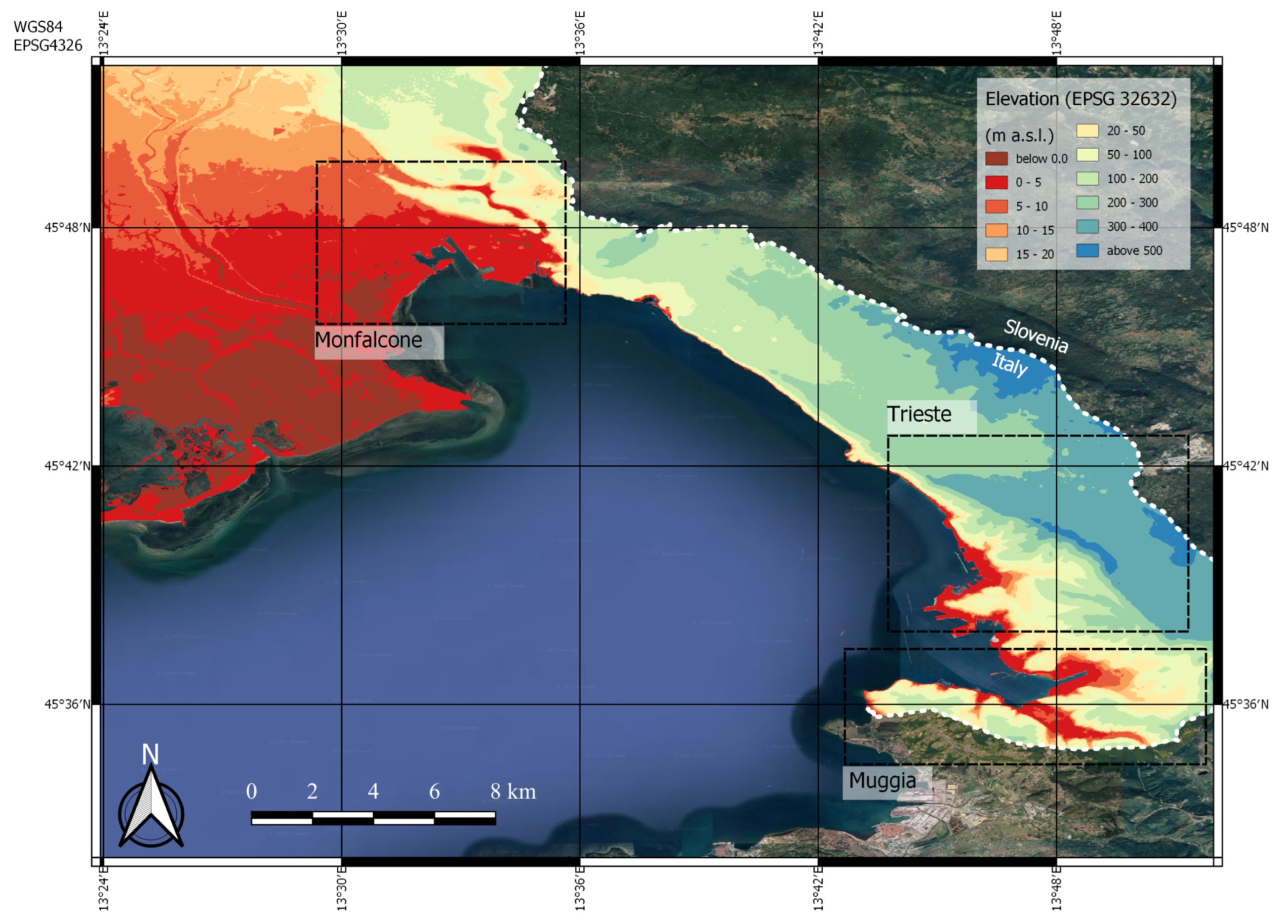
3.1. Study Area
Digital Elevation Model in the Study Area
3.2. Flood Conditioning Factors
- denotes the Water Velocity (in m/s) at the ith pixel;
- denotes the Water Depth (in m) at the ith pixel;
- denotes the slope (in decimals) per pixel;
- L
- denotes the resolution (in m) of each pixel;
- denotes the Manning Roughness (Gauckler–Manning–Strickler) coefficient (in s/m), which also depends on the land use and thus can be related by the Corine Land Cover index, indicating the surface roughness per pixel.
3.3. Satellite Imagery Analysis
- Apply Orbit File: The operation of applying a precise orbit available in SNAP allows the automatic download and update of the orbit state vectors for each SAR scene in its product metadata, providing an accurate satellite position and velocity information.
- Thermal Noise Removal: Reduces noise effects in the inter-sub-swath texture, in particular normalizing the backscatter signal within the entire Sentinel-1 scene and resulting in reduced discontinuities between sub-swaths for scenes in multi-swath acquisition modes.
- Subset: The initial product is cropped, so it contains only the lake we want to observe. Some balance between the inundated and non-inundated areas is desired.
- Radiometric calibration: Fixes the uncertainty in the radiometric resolution of satellite sensor. The pixel values can be directly related to the radar backscatter of the scene. The information required to apply the calibration equation is included within the Sentinel-1 GRD product.
- Speckle noise removal: Removes the salt-and-pepper-like pattern noise that is caused by the interference of electromagnetic waves. The “Lee Sigma” filter of Lee (1981) [47] with a 5 × 5 filter size is used to filter the intensity data. As noted by Jong-Sen Lee et al. (2009) [48], this step is essential in almost any analysis of radar images due to the speckle noise aggravation of the interpretation process.
- Terrain correction: Projects the pixels onto a map system (WGS84 was selected) and re-samples it to a 10 m spatial resolution. In addition, topographic corrections with a Shuttle Radar Topography Mission (SRTM) digital elevation model (DEM) are performed. Corrects the distortions over the areas of the terrain.
- Linear to Decibel (dB): The dynamic range of the backscatter intensity of the transmitted radar signal values is usually a few orders of magnitudes. Thus, these values are converted from linear scale to logarithmic scale, leading to an easier to manipulate histogram, also making water and dry areas more distinctive.
3.4. Machine Learning Techniques
- Support Vector Machine—SVM: Support Vector Machine (SVM) Classifier [49] represents a supervised machine learning technique that exploits the abilities of hyperplanes, reshaping the nonlinear world into linear in order to classify the features. Hyperplane is a decision plane that aims to separate a set of objects and label them into different classes. SVM consists of a method aiming to separate the features in more efficient way using hyperplanes.
- Naive Bayes—NB: According to the Bayes Theorem, we deployed the statistical classification technique, Naïve Bayes (NB) classifier. This classifier belongs to the group of supervised learning algorithms and happens to be one of the simplest with high accuracy and speed, especially when it collocates with large datasets. NB is using a classifier model, which is assigning class labels into the problem events, represented as vectors of feature events, where a set is used to annotate the class labels.
- Random Forest—RF: The Random Forest (RF) [50] is a well-known ensemble machine learning method either for classification or regression. The objective of this classification technique is to compare and analyze the dataset variables to define new weights for each factor. In our case of study, the RF model exploits decision trees in order to calculate and estimate the connection between Flood Hazard Index labeling and Flood feature factors values, focusing on the end to classify each vector of values into a predicted label. RF is simple, fast, able to handle large datasets, has generally high outcome through randomization and is applicable to multiclass algorithm characteristics.
- Neural Network—NN: Neural Networks can be portrayed as the hierarchical multilevel relationships between neurons in a network of neurons similar to the function of the brain. The neurons implement a feedback mechanism with each other, transmitting the necessary signals to the next levels, based on the received input received from the respective previous levels, reaching one or more final results.
3.5. Model Evaluation Metrics
- Confusion matrix: A confusion matrix is a table (Table 1) that presents the results from classifiers using some specific terms, such as “True positives (TP)", the predicted and actually positive result; “False positives (FP)”, the predicted positive but actually negative result; “True negatives (TN)”, the predicted and actually negative result; and “False negatives (FN)”, the predicted negative but actually positives.
- Accuracy: Accuracy is the most commonly used percentage metric for machine learning models judging the accuracy of the results and can be calculated using confusion matrix terms:
- Precision: Precision answers the question of what analogy of the positive results was in fact correct and can be calculated using:
- Recall: Recall, on the other hand, answers the question of what analogy of true positives was identified correctly and can be calculated using:
- F1-score: F1-Score is a measure to evaluate classification systems and is a way to combine the precision and recall results. It can be described as the harmonic mean of precision and recall and can be calculated using:
- Cross-Validation k-fold: Cross-validation is a statistical method of evaluating machine learning models, where it divides the dataset into random K-segments in order to use them for model training, and comparing them, we select the best model. The process of cross-validation has a single parameter k, which refers to the number of segments that will randomly separate each set of data. In our case, k is equal to 10, and we choose the best model using the average result per training.
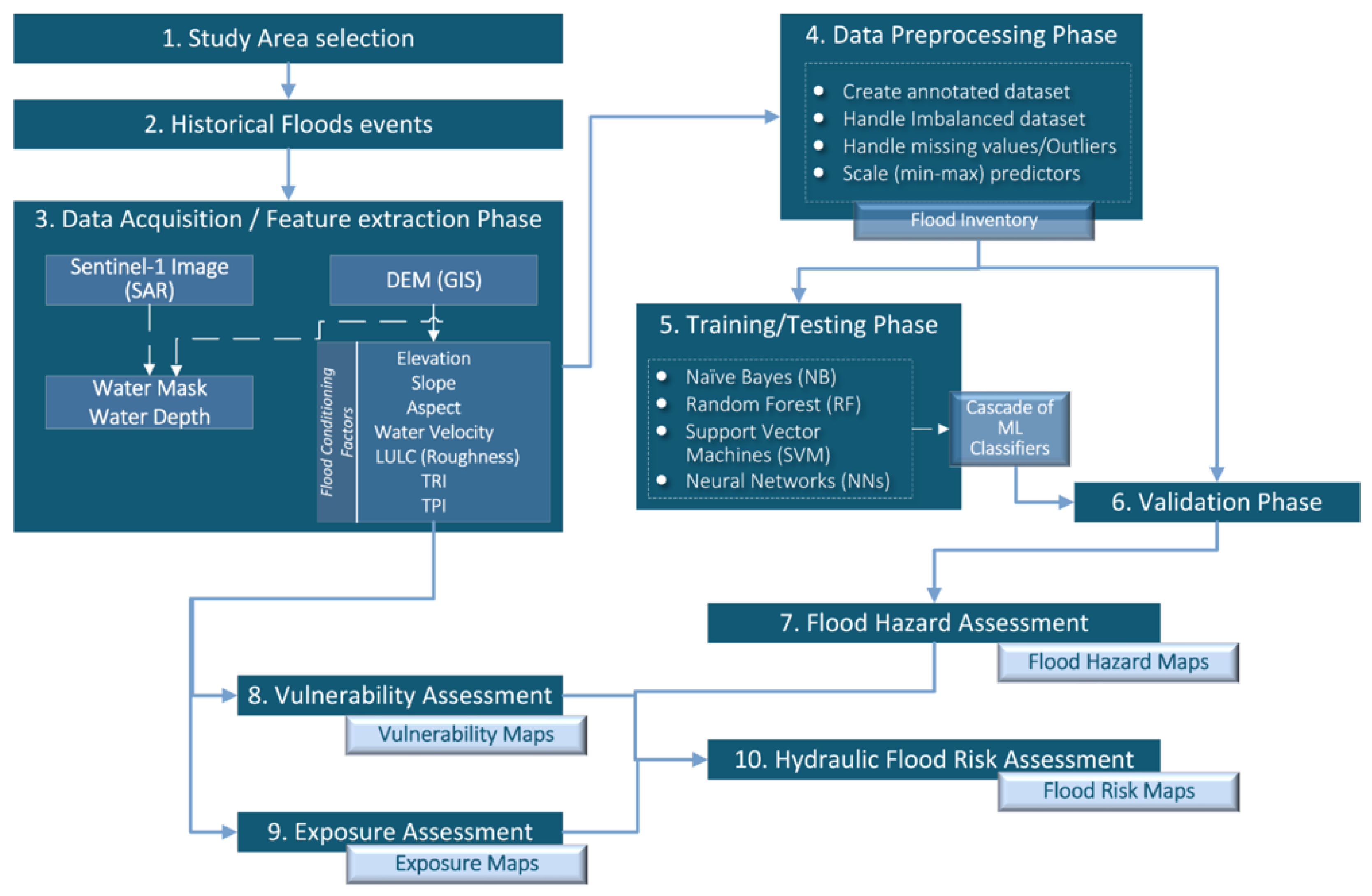
4. Methodology
4.1. Dynamic Flood Hazard Assessment Algorithm
4.1.1. Study Area and Historical Flood Events
4.1.2. Data Acquisition and Feature Extraction
4.1.3. Data Preprocessing
- Create annotated dataset: Upgrade the data set by adding a target variable so that Machine Learning techniques can be applied. Our goal is to create machine learning models enable to assess the flood hazard level and which rely on the flood conditioning factors and the real-time analysis of satellite imagery. Hence, the target-variable should be the “Flood Hazard” that receives three potential values, namely, Moderate (Low) Hazard, Medium Hazard and High Hazard. To annotate the dataset, the following rule will be applied [44,55]:
It should be mentioned here that the above rule is based on a hypothesis of medium probability of the flood, which has a 100-year return period in the study area.If m/s and Then Moderate Hazard Else IfandThen Medium Hazard Else IfandThen High Hazard - Handle Imbalanced dataset: Due to the facts that inundated areas usually are a quite small portion of the whole region of interest and furthermore floods are a quite rare extreme event, then it is expected the majority of entries in the “Flood Hazard” will belong to the Moderate Hazard class causing an imbalanced dataset. Hence, the machine learning models will be biased to the majority class. To tackle this issue, a random sampling is performed, and a portion of the majority class is selected equal to the amount of data that belong to the other two classes.
- Handle missing or extreme values: Pixels with missing values or extreme values that indicate areas that are out of the interest, e.g., inside the sea, should be detected and removed from the analysis.
- Data Normalisation: The aim is to eliminate the numerical differences between the features and transform them to the same range. Machine learning models require that the input data are normalized using the same range, since the bias may occur in the results due to the bigger magnitude of the initial untransformed data. Hence, the min–max scaler is utilised that transforms each one of the input features (predictors) to min–max scale (i.e., [0, 1] scale). The formula is given as follows:where X is the normalized data, x is the raw data, is the minimum value of each feature vector and is the maximum value of each feature vector.
4.1.4. Training, Testing and Validation
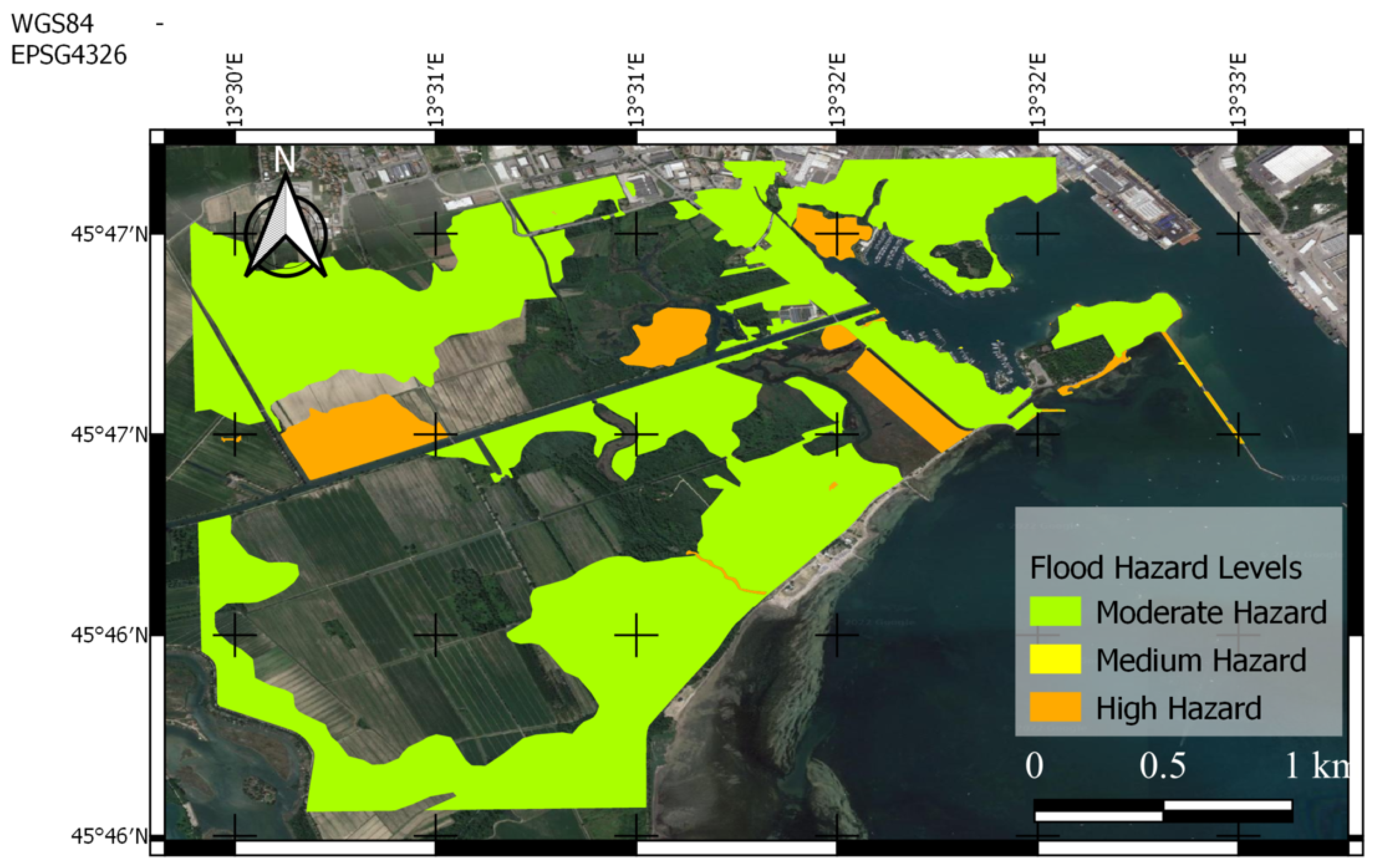
4.1.5. Flood Hazard Assessment and Mapping
4.2. Dynamic Flood Risk Assessment Algorithm
4.2.1. Vulnerability Estimation
- Vulnerability of people (Vp): The physical vulnerability associated with people considers the values of flow velocity (Water Velocity—v) and Water Depth (h) that produce “instability” with respect to remaining in an upright position [58]. FRMP proposes a semi-quantitative equation that links a flood hazard index, referred to as the Flood Hazard Rating (FHR), to h, v and a factor related to the amount of transported debris, i.e., the Debris Factor (DF). According to this algorithm, the land use type classes are grouped in order to calculate the Debris Factor (DF) concerning the possibility of floating materials which can harm the population.After the calculation of DF, the estimation of the Flood Hazard Rating (FHR) is carried out by utilising the Water Depth and Water Velocity according to the following formula:where h is the Water Depth, v is the Water Velocity and DF is the Debris Factor. Vp is estimated according to FHR (Table 2).
- Vulnerability of economic activities (Ve): The vulnerability associated with economic activities considers buildings, network infrastructure and agricultural areas [58]. It is a pixel-by-pixel function of the Water Depth (height) and Water Velocity (flow velocity). The vulnerability function depends on the specific nature of the assets and thus different functions are applied to land use types.
- Vulnerability of environments and cultural-archaeological assets and protected areas (Va): Environmental flood susceptibility is described using contamination/pollution and erosion as indicators. Contamination is caused by industry, animal/human waste and stagnant flooded waters. Erosion can produce disturbance to the land surface and to vegetation but can also damage infrastructure [58]. From AAWA’s FRMP [44,55], the value of Va in certain land use is 1, while assuming a residual Va value for all others.
4.2.2. Exposure Estimation
- Exposure of people (Ep): First step to calculating the Ep is to estimate the population of the area of interest per pixel, which is divided into census areas by the Italian national Institute of Statistics (ISTAT). The dataset of population is given to us via shapefiles, which are a form of geospatial vectors, so we can calculate per pixel according to geolocation data. The calculation of Ep can be produced by:where is a factor characterizing the density of the population in relation to the number of people present. For the population estimations in specific areas, census data have been employed. is the proportion of time spent in different locations (e.g., houses and schools) using the land use classes.
- Exposure of economic activity (Ee): The Ee calculation depends solely on the land use of the area of interest.
- Exposure of environment and cultural elements (Ea): As with Ee, exposure of environment and cultural elements, Ea is estimated solely by land use.
4.2.3. Hydraulic Flood Risk Assessment
- = 10, if there are inhabitants;
- = 1, if there are economic activities;
- = 1, if there are environments and cultural-archaeological assets and protected areas.
5. Results and Discussion
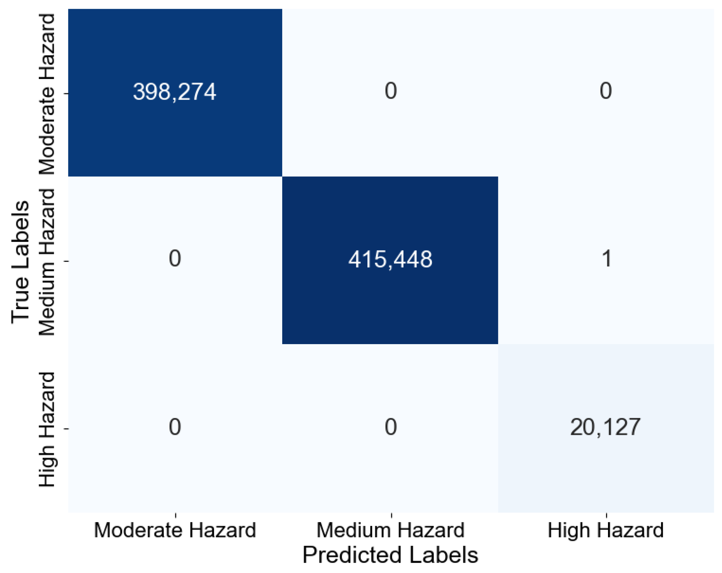
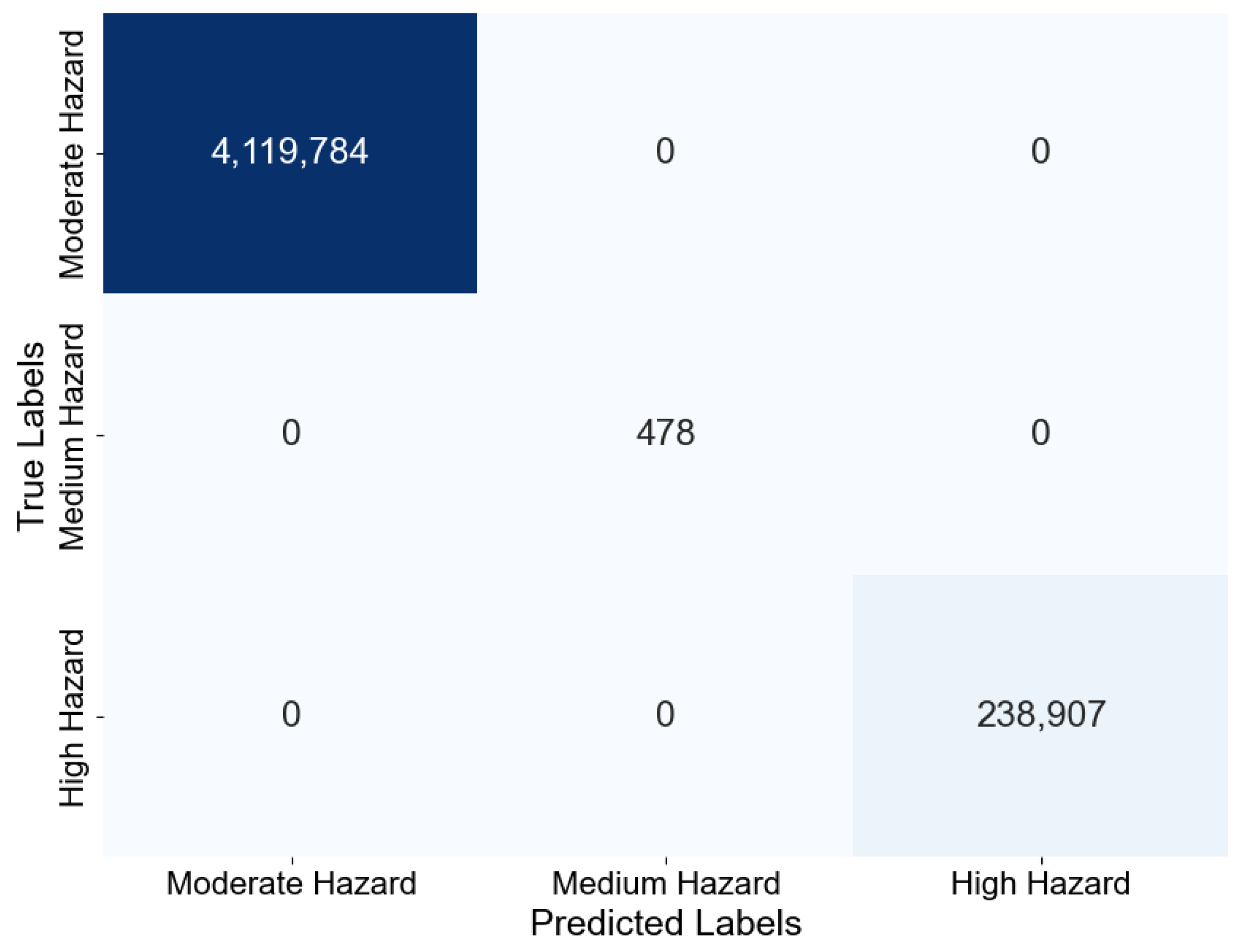
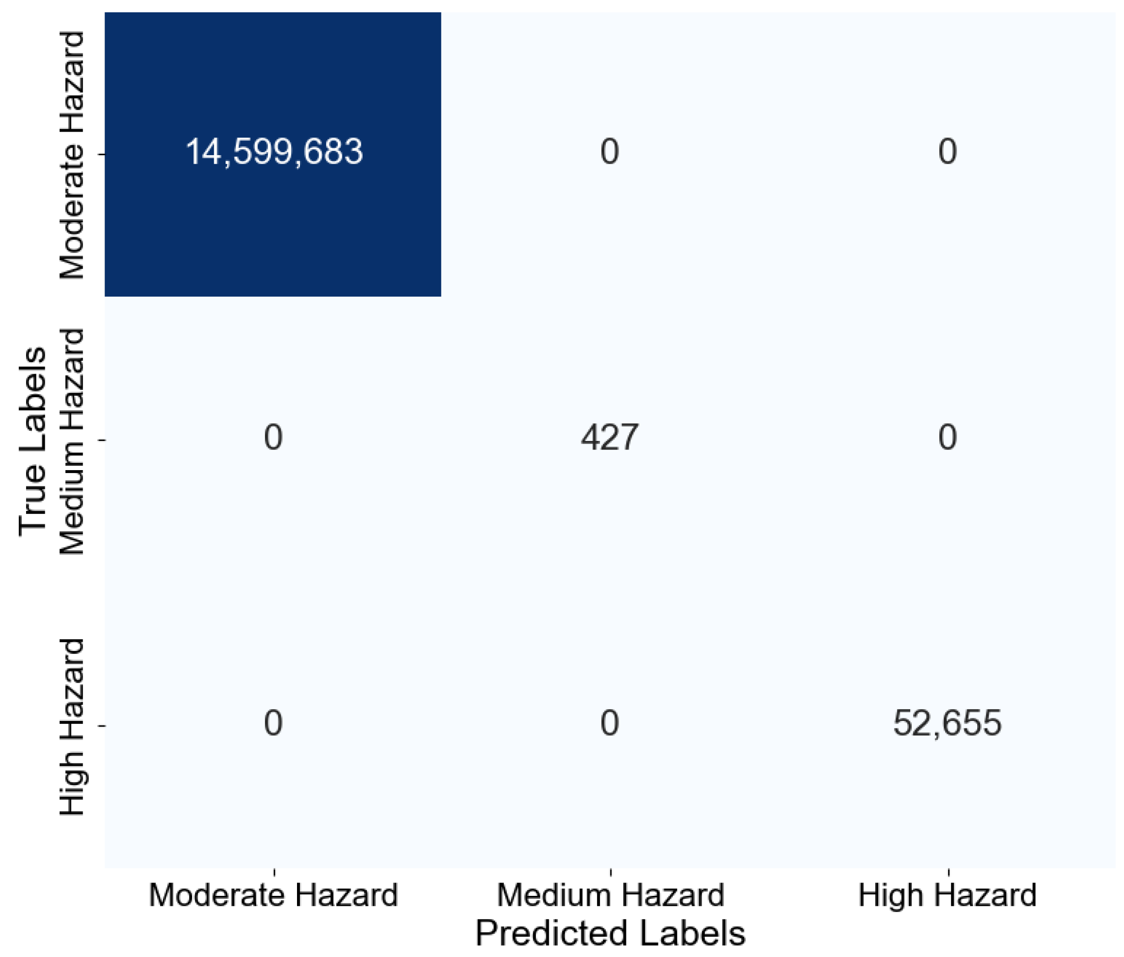
5.1. Evaluation of Dynamic Flood Hazard/Risk Algorithm
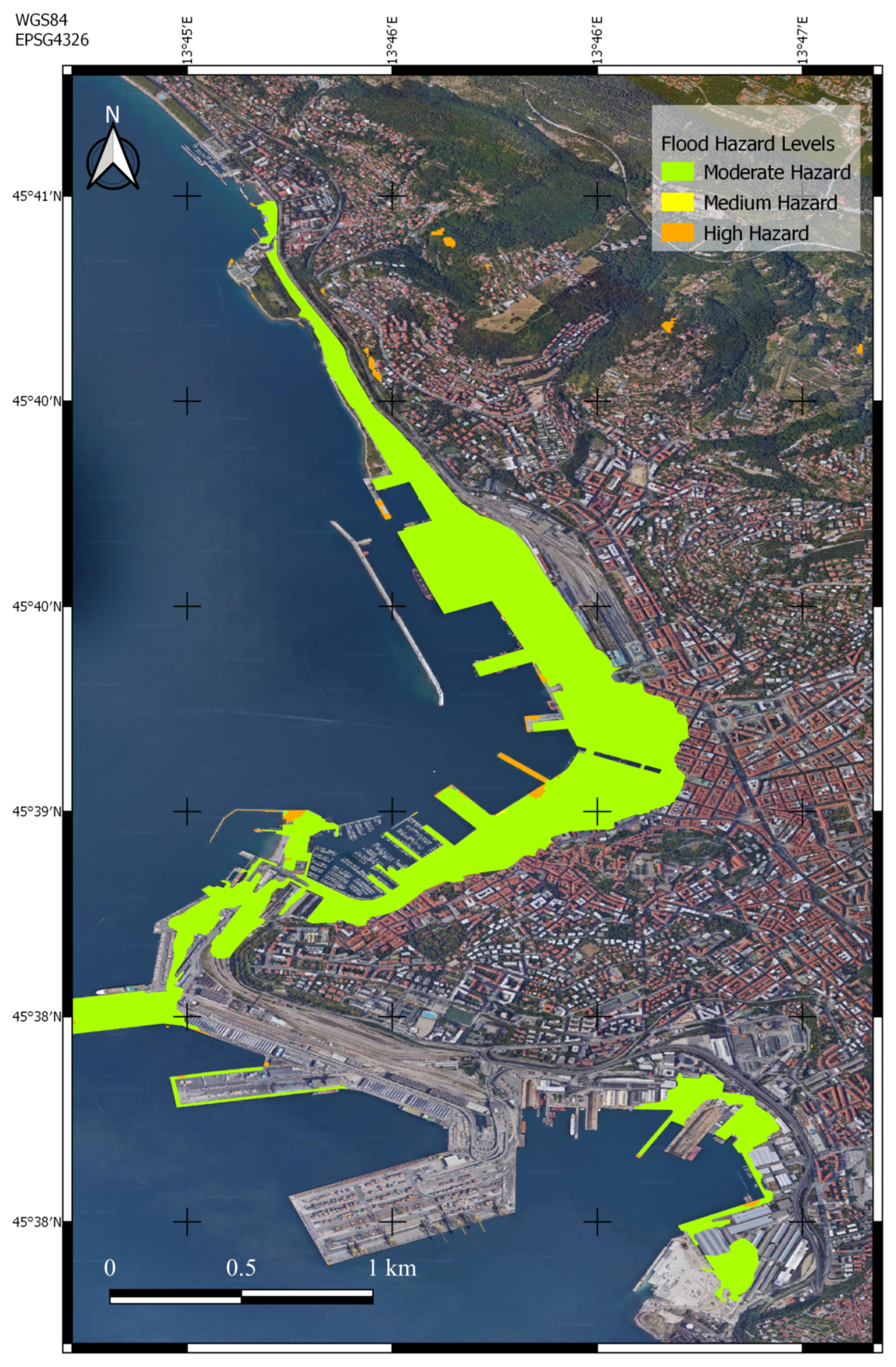
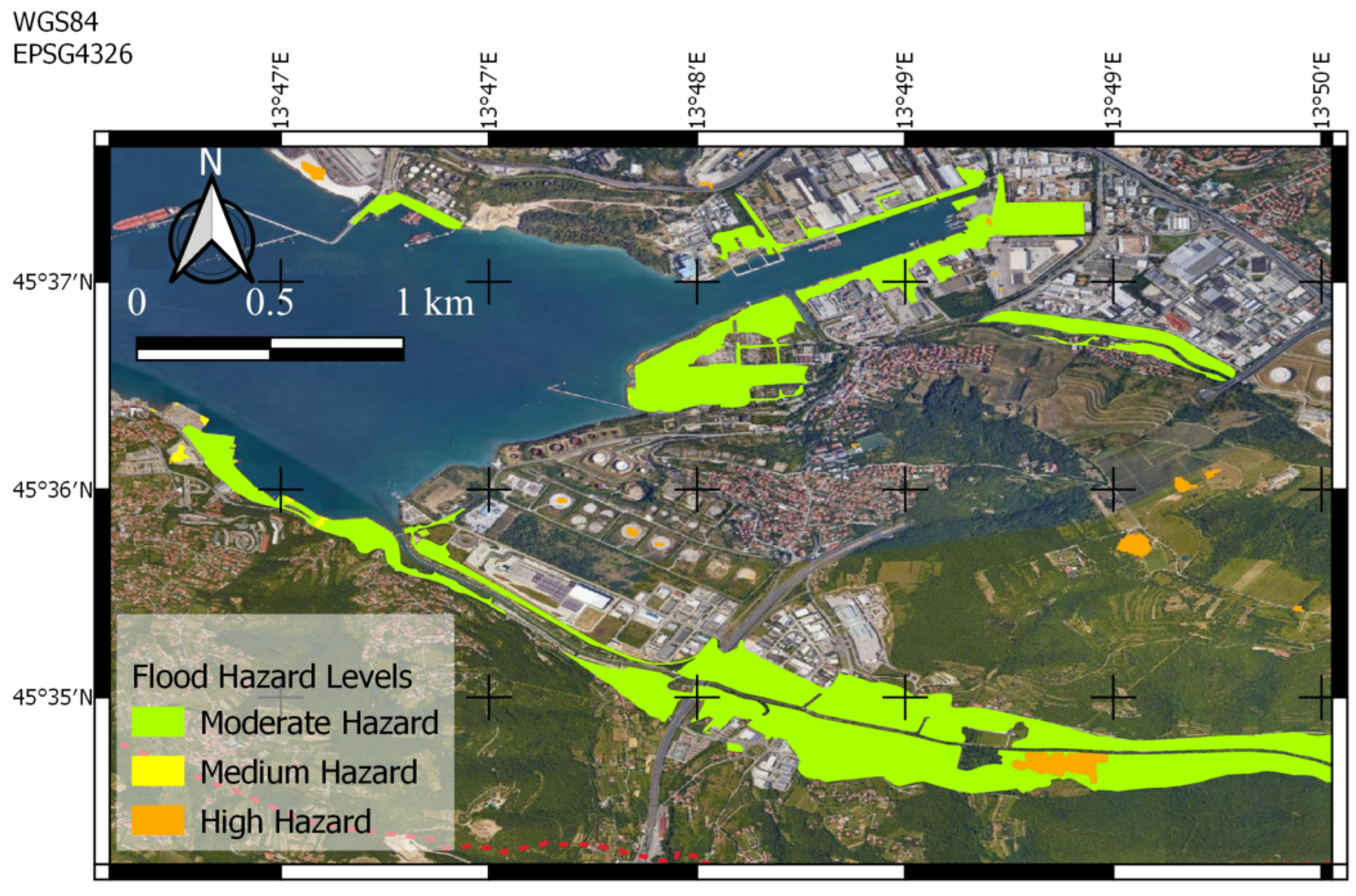
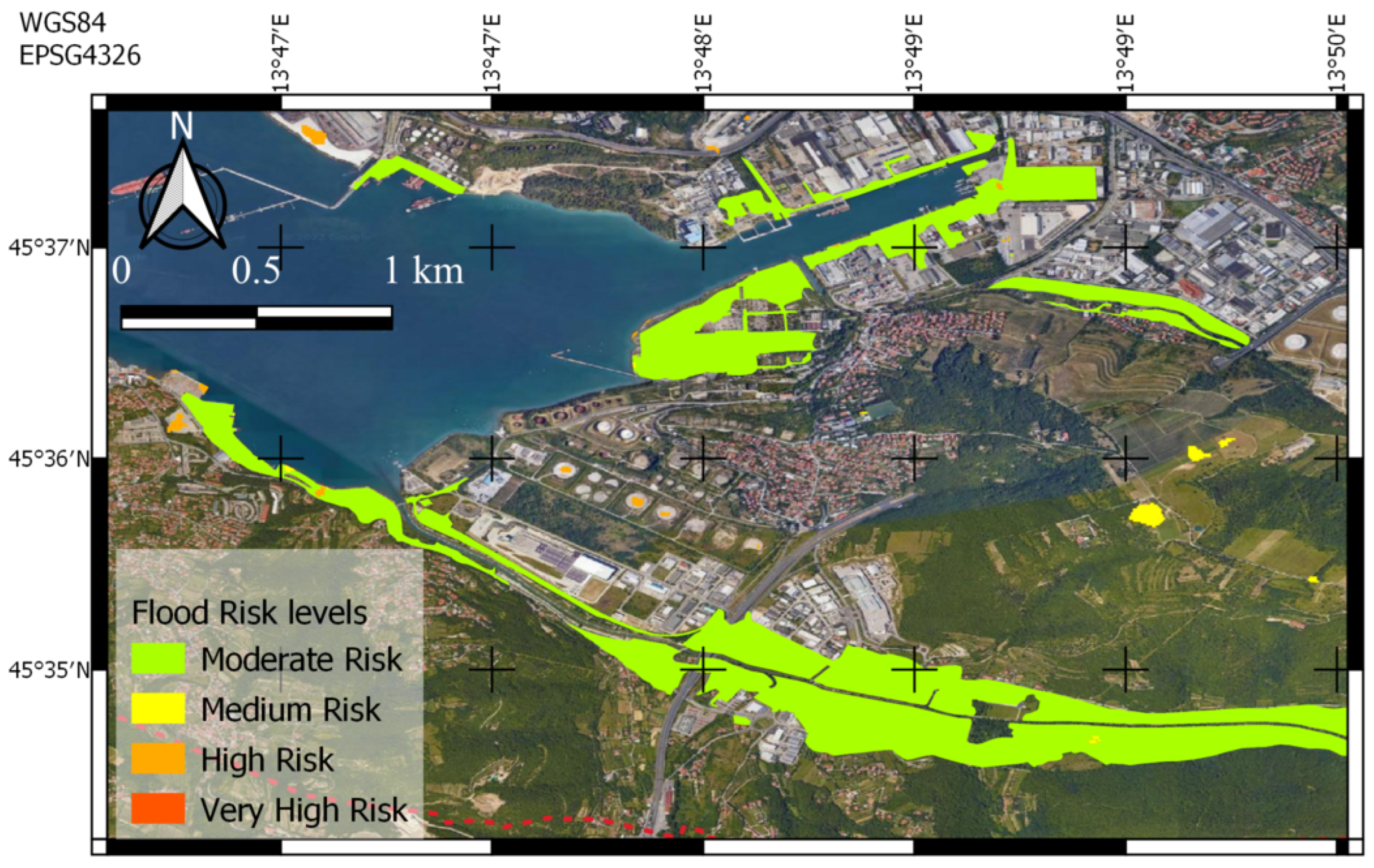
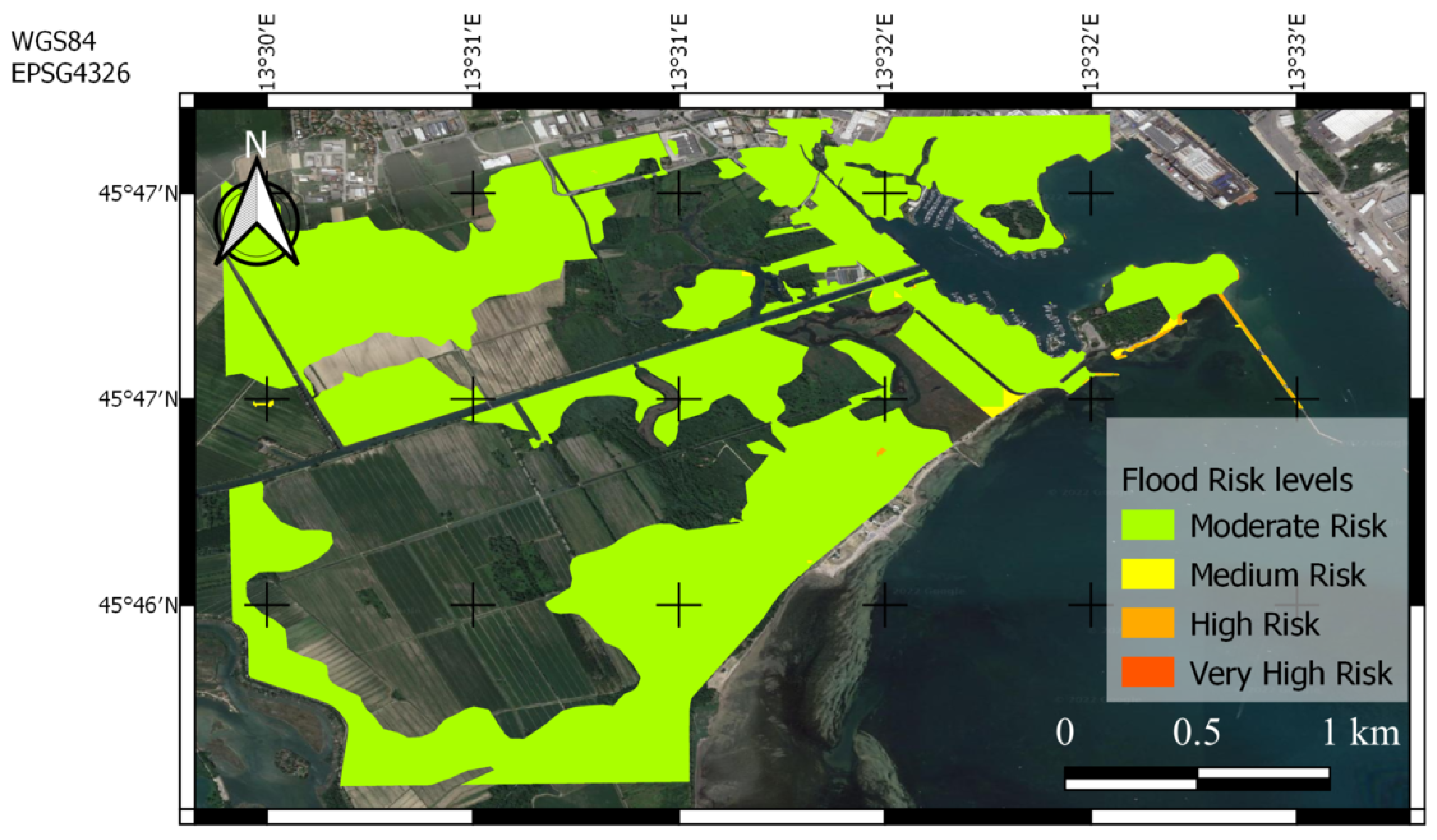
5.1.1. Trieste, 23 September 2019
5.1.2. Muggia, 29 October 2018
5.1.3. Monfalcone, 24 September 2019
5.2. Discussion
6. Conclusions
- The domain lack of annotated datasets for the training and evaluation of the machine learning techniques able to detect and monitor the flood event by using remote sensing techniques;
- The low temporal frequency of satellite imagery acquisition, which hinders the real-time monitoring of an evolving flood.
Author Contributions
Funding
Institutional Review Board Statement
Informed Consent Statement
Data Availability Statement
Conflicts of Interest
Abbreviations
| AAWA | Alto Adriatico Water Authority |
| AHP | Analytical Hierarchy Process |
| AoI | Area of Interest |
| ANNs | Artificial Neural Networks |
| CART | Classification and Regression Trees |
| CRCL | Crisis Classification |
| CLC | Corine Landcover Codex |
| CNN | Convolutional Neural Network |
| DEM | Digital Elevation Model |
| DNN | Deep Neural Network |
| DRR | Disaster Risk Reduction |
| EaR | Elements at Risk |
| Ep | Exposure of people |
| Ee | Exposure of economic activity |
| Ea | Exposure of environment and cultural elements |
| FFPI | Flash-Flood Potential Index |
| FHR | Flood Hazard Rating |
| FR | Frequency Ratio |
| FRMP | Flood Risk Management Plan |
| GIS | Geographical Information System |
| LIDAR | Laser Imaging, Detection And Ranging |
| LR | Logistic Regression |
| LULC | Land Use Land Cover |
| MDA | Multivariate Discriminant Analysis |
| NNs | Neural Networks |
| RF | Random Forest |
| SAR | Synthetic Aperture Radar |
| SNAP | Sentinel Application Platform |
| SVMs | Support Vector Machines |
| TRI | Terrain Ruggedness Index |
| TWI | Topographic Wetness Index |
| UAVs | Unmanned Aerial Vehicles |
| Vp | Vulnerability of people |
| Ve | Vulnerability of economic activities |
| Va | Vulnerability of environments and cultural-archaeological assets and protected areas |
References
- Pinos, J.; Quesada-Román, A. Flood Risk-Related Research Trends in Latin America and the Caribbean. Water 2022, 14, 10. [Google Scholar] [CrossRef]
- van Loenhout, J.; McClean, D. Human Cost of Disasters. An Overview of the Last 20 Years 2000–2019; UN Office for Disaster Risk Reduction (UNDRR) and Centre for Research on the Epidemiology of Disasters (CRED): Brussels, Belgium, 2020. [Google Scholar]
- Quesada-Román, A.; Ballesteros-Cánovas, J.A.; Granados-Bolaños, S.; Birkel, C.; Stoffel, M. Dendrogeomorphic reconstruction of floods in a dynamic tropical river. Geomorphology 2020, 359, 107133. [Google Scholar] [CrossRef]
- Quesada-Román, A.; Ballesteros-Cánovas, J.A.; Granados-Bolaños, S.; Birkel, C.; Stoffel, M. Improving regional flood risk assessment using flood frequency and dendrogeomorphic analyses in mountain catchments impacted by tropical cyclones. Geomorphology 2022, 396, 108000. [Google Scholar] [CrossRef]
- Said, N.; Ahmad, K.; Riegler, M.; Pogorelov, K.; Hassan, L.; Ahmad, N.; Conci, N. Natural disasters detection in social media and satellite imagery: A survey. Multimed. Tools Appl. 2019, 78, 31267–31302. [Google Scholar] [CrossRef] [Green Version]
- Yu, M.; Yang, C.; Li, Y. Big Data in Natural Disaster Management: A Review. Geosciences 2018, 8, 165. [Google Scholar] [CrossRef] [Green Version]
- Arshad, B.; Ogie, R.; Barthélemy, J.; Pradhan, B.; Verstaevel, N.; Perez, P. Computer Vision and IoT-Based Sensors in Flood Monitoring and Mapping: A Systematic Review. Sensors 2019, 19, 5012. [Google Scholar] [CrossRef] [PubMed] [Green Version]
- Dottori, F.; Kalas, M.; Salamon, P.; Bianchi, A.; Thielen Del Pozo, J.; Feyen, L. A near real-time procedure for flood hazard mapping and risk assessment in Europe. In Proceedings of the 36th IAHR World Congress, The Hague, The Netherlands, 28 June–3 July 2015; International Association for Hydro-Environment Engineering and Research (IAHR): Thessaloniki, Greece, 2015; pp. 4968–4975. [Google Scholar]
- EXCIMAP. Atlas of Flood Maps. Examples from 19 European Countries, USA and Japan; Ministerie V&W: Den Haag, The Netherlands, 2007; p. 197. [Google Scholar]
- EXCIMAP. Handbook on Good Practices for Flood Mapping in Europe; European Commision: Den Haag, The Netherlands, October 2007.
- Constantinescu, G.; Garcia, M.; Hanes, D. River Flow 2016: Iowa City; CRC Press: Boca Raton, FL, USA, 2016. [Google Scholar] [CrossRef]
- Ekeu-wei, I.; Blackburn, G. Applications of Open-Access Remotely Sensed Data for Flood Modelling and Mapping in Developing Regions. Hydrology 2018, 5, 39. [Google Scholar] [CrossRef] [Green Version]
- Díez-Herrero, A.; Lain-Huerta, L.; Llorente, M. A Handbook on Flood Hazard Mapping Methodologies; Geological Survey of Spain: Madrid, Spain, 2009. [Google Scholar]
- Spachinger, K.; Dorner, W.; Metzka, R.; Serrhini, K.; Fuchs, S. Flood Risk and Flood hazard maps—Visualisation of hydrological risks. IOP Conf. Ser. Earth Environ. Sci. 2008, 4, 012043. [Google Scholar] [CrossRef] [Green Version]
- Wagenaar, D.; Curran, A.; Balbi, M.; Bhardwaj, A.; Soden, R.; Hartato, E.; Mestav Sarica, G.; Ruangpan, L.; Molinario, G.; Lallemant, D. Invited perspectives: How machine learning will change flood risk and impact assessment. Nat. Hazards Earth Syst. Sci. 2020, 20, 1149–1161. [Google Scholar] [CrossRef]
- Global Facility for Disaster Reduction and Recovery (GFDRR). Machine Learning for Disaster Risk Management. 2018. Available online: https://www.gfdrr.org/sites/default/files/publication/181222_WorldBank_DisasterRiskManagement_Ebook_D6.pdf (accessed on 17 January 2020).
- Klemas, V. Remote Sensing of Floods and Flood-Prone Areas: An Overview. J. Coast. Res. 2015, 31, 1005–1013. [Google Scholar] [CrossRef]
- Kuenzer, C.; Guo, H.; Huth, J.; Leinenkugel, P.; Li, X.; Dech, S. Flood Mapping and Flood Dynamics of the Mekong Delta: ENVISAT-ASAR-WSM Based Time Series Analyses. Remote Sens. 2013, 5, 687–715. [Google Scholar] [CrossRef] [Green Version]
- Quesada-Román, A.; Villalobos-Chacón, A. Flash flood impacts of Hurricane Otto and hydrometeorological risk mapping in Costa Rica. Geogr. Tidsskr.-Dan. J. Geogr. 2020, 120, 142–155. [Google Scholar] [CrossRef]
- Van Ackere, S.; Verbeurgt, J.; De Sloover, L.; Gautama, S.; Wulf, A.; De Maeyer, P. A Review of the Internet of Floods: Near Real-Time Detection of a Flood Event and Its Impact. Water 2019, 11, 2275. [Google Scholar] [CrossRef] [Green Version]
- Costache, R.; Pham, Q.B.; Sharifi, E.; Linh, N.T.T.; Abba, S.; Vojtek, M.; Vojteková, J.; Nhi, P.T.T.; Khoi, D.N. Flash-Flood Susceptibility Assessment Using Multi-Criteria Decision Making and Machine Learning Supported by Remote Sensing and GIS Techniques. Remote Sens. 2020, 12, 106. [Google Scholar] [CrossRef] [Green Version]
- Pham, B.T.; Phong, T.V.; Nguyen, H.D.; Qi, C.; Al-Ansari, N.; Amini, A.; Ho, L.S.; Tuyen, T.T.; Yen, H.P.H.; Ly, H.B.; et al. A Comparative Study of Kernel Logistic Regression, Radial Basis Function Classifier, Multinomial Naïve Bayes, and Logistic Model Tree for Flash Flood Susceptibility Mapping. Water 2020, 12, 239. [Google Scholar] [CrossRef] [Green Version]
- Pham, B.; Avand, M.; Janizadeh, S.; Tran, P.; Al-Ansari, N.; Lanh, H.; Das, S.; Le, H.; Amini, A.; Bozchaloei, S.; et al. GIS Based Hybrid Computational Approaches for Flash Flood Susceptibility Assessment. Water 2020, 12, 683. [Google Scholar] [CrossRef] [Green Version]
- Tehrany, M.; Pradhan, B.; Mansor, S.; Ahmad, N. Flood susceptibility assessment using GIS-based support vector machine model with different kernel types. Catena 2015, 125, 91–101. [Google Scholar] [CrossRef]
- Mind’je, R.; Li, L.; Amanambu, A.; Nahayo, L.; Nsengiyumva, J.B.; Gasirabo, A.; Mindje, M. Flood susceptibility modeling and hazard perception in Rwanda. Int. J. Disaster Risk Reduct. 2019, 38, 101211. [Google Scholar] [CrossRef]
- Rahman, M.; Ningsheng, C.; Islam, M.M.; Dewan, A.; Iqbal, J.; Washakh, R.M.A.; Shufeng, T. Flood susceptibility assessment in Bangladesh using machine learning and multi-criteria decision analysis. Earth Syst. Environ. 2019, 3, 585–601. [Google Scholar] [CrossRef]
- Saleem, N.; Huq, M.E.; Twumasi, N.Y.D.; Javed, A.; Sajjad, A. Parameters Derived from and/or Used with Digital Elevation Models (DEMs) for Landslide Susceptibility Mapping and Landslide Risk Assessment: A Review. ISPRS Int. J. Geo-Inf. 2019, 8, 545. [Google Scholar] [CrossRef] [Green Version]
- Vojtek, M.; Vojteková, J. Flood Susceptibility Mapping on a National Scale in Slovakia Using the Analytical Hierarchy Process. Water 2019, 11, 364. [Google Scholar] [CrossRef] [Green Version]
- Quesada-Román, A. Landslide and flood zoning using geomorphological analysis in a dynamic basin of Costa Rica. Cartogr. Mag. 2021, 102, 125–138. [Google Scholar] [CrossRef]
- Swain, K.C.; Singha, C.; Nayak, L. Flood Susceptibility Mapping through the GIS-AHP Technique Using the Cloud. ISPRS Int. J. Geo-Inf. 2020, 9, 720. [Google Scholar] [CrossRef]
- Jacinto, R.; Grosso, N.; Reis, E.; Dias, L.; Santos, F.D.; Garrett, P. Continental Portuguese Territory Flood Susceptibility Index – contribution to a vulnerability index. Nat. Hazards Earth Syst. Sci. 2015, 15, 1907–1919. [Google Scholar] [CrossRef] [Green Version]
- Giordan, D.; Notti, D.; Villa, A.; Zucca, F.; Calò, F.; Pepe, A.; Dutto, F.; Pari, P.; Baldo, M.; Allasia, P. Low cost, multiscale and multi-sensor application for flooded area mapping. Nat. Hazards Earth Syst. Sci. 2018, 18, 1493–1516. [Google Scholar] [CrossRef] [Green Version]
- Ahamed, A.; Bolten, J.; Doyle, C.; Fayne, J. Near Real-Time Flood Monitoring and Impact Assessment Systems. In Remote Sensing of Hydrological Extremes; Lakshmi, V., Ed.; Springer International Publishing: Cham, Switzerlands, 2017; pp. 105–118. [Google Scholar] [CrossRef]
- Kwak, Y.j. Nationwide Flood Monitoring for Disaster Risk Reduction Using Multiple Satellite Data. ISPRS Int. J. Geo-Inf. 2017, 6, 203. [Google Scholar] [CrossRef]
- Erdelj, M.; Natalizio, E.; Chowdhury, K.R.; Akyildiz, I.F. Help from the Sky: Leveraging UAVs for Disaster Management. IEEE Pervasive Comput. 2017, 16, 24–32. [Google Scholar] [CrossRef]
- Kyrkou, C.; Theocharides, T. Deep-Learning-Based Aerial Image Classification for Emergency Response Applications Using Unmanned Aerial Vehicles. In Proceedings of the 2019 IEEE/CVF Conference on Computer Vision and Pattern Recognition Workshops (CVPRW), Long Beach, CA, USA, 16–17 June 2019; pp. 517–525. [Google Scholar] [CrossRef] [Green Version]
- Granados-Bolaños, S.; Quesada-Román, A.; Alvarado, G.E. Low-cost UAV applications in dynamic tropical volcanic landforms. J. Volcanol. Geotherm. Res. 2021, 410, 107143. [Google Scholar] [CrossRef]
- Nandi, A.; Mandal, A.; Wilson, M.; Smith, D. Flood hazard mapping in Jamaica using principal component analysis and logistic regression. Environ. Earth Sci. 2016, 75, 465. [Google Scholar] [CrossRef]
- Choubin, B.; Moradi, E.; Golshan, M.; Adamowski, J.; Sajedi-Hosseini, F.; Mosavi, A. An ensemble prediction of flood susceptibility using multivariate discriminant analysis, classification and regression trees, and support vector machines. Sci. Total Environ. 2019, 651, 2087–2096. [Google Scholar] [CrossRef]
- Rizeei, H.; Pradhan, B.; Nampak, H.; Ahmad, N.; Ghazali, A. Ensemble machine-learning-based geospatial approach for flood risk assessment using multi- sensor remote-sensing data and GIS Ensemble machine-learning-based geospatial approach for flood risk assessment using multi-sensor remote-sensing data and GIS. Geomat. Nat. Hazards Risk 2017, 8, 1080–1102. [Google Scholar] [CrossRef] [Green Version]
- Opella, J.M.A.; Hernandez, A.A. Developing a Flood Risk Assessment Using Support Vector Machine and Convolutional Neural Network: A Conceptual Framework. In Proceedings of the 2019 IEEE 15th International Colloquium on Signal Processing Its Applications (CSPA), Penang, Malaysia, 8–9 March 2019; pp. 260–265. [Google Scholar]
- Mpakratsas, M.; Moumtzidou, A.; Gialampoukidis, I.; Vrochidis, S.; Kompatsiaris, I. A Deep Neural Network Slope Reduction Model on Sentinel-1 Images for Water Mask Extraction. In Proceedings of the 40th Asian Conference on Remote Sensing (ACRS 2019), Daejeon, Korea, 14–18 October 2019. [Google Scholar] [CrossRef]
- Friuli Venezia Giulia Region. Piano Stralcio per l’assetto Piano Stralcio per l’assetto Idrogeologico dei Bacini di Interesse Regionale (Bacini Idrografici dei Tributari della Laguna di Marano—Grado, ivi Compresa la Laguna Medesima, del Torrente Slizza e del Levante). 2016. Available online: https://www.regione.fvg.it/rafvg/export/sites/default/RAFVG/ambiente-territorio/geologia/FOGLIA24/allegati/PAIR_Allegato_01_relazione_illustrativa.pdf (accessed on 5 November 2021).
- Eastern Alps River Basin District Authority—AAWA. Flood Risk Management Plan of the Eastern Alps Hydrographic District. Decree of the President of the Italian Council of Ministers of 27 October 2016. 2017. Available online: https://va.minambiente.it/en-GB/Oggetti/Info/1456 (accessed on 5 November 2021).
- Rahmati, O.; Yousefi, S.; Kalantari, Z.; Uuemaa, E.; Teimurian, T.; Keesstra, S.; Pham, T.D.; Tien Bui, D. Multi-Hazard Exposure Mapping Using Machine Learning Techniques: A Case Study from Iran. Remote Sens. 2019, 11, 1943. [Google Scholar] [CrossRef] [Green Version]
- Filipponi, F. Sentinel-1 GRD Preprocessing Workflow. Proceedings 2019, 18, 11. [Google Scholar] [CrossRef] [Green Version]
- Lee, J.S. Refined filtering of image noise using local statistics. Comput. Graph. Image Process. 1981, 15, 380–389. [Google Scholar] [CrossRef]
- Lee, J.S.; Wen, J.H.; Ainsworth, T.L.; Chen, K.S.; Chen, A.J. Improved sigma filter for speckle filtering of SAR imagery. IEEE Trans. Geosci. Remote Sens. 2008, 47, 202–213. [Google Scholar]
- Cortes, C.; Vapnik, V. Support-vector networks. Mach. Learn. 1995, 20, 273–297. [Google Scholar] [CrossRef]
- Tin Kam, H. Random decision forests. In Proceedings of the 3rd International Conference on Document Analysis and Recognition, Montreal, QC, Canada, 14–16 August 1995; Volume 1, pp. 278–282. [Google Scholar] [CrossRef]
- Kron, W. Flood Risk = Hazard • Values • Vulnerability. Water Int. 2005, 30, 58–68. [Google Scholar] [CrossRef]
- Wannous, C.; Velasquez, G. United Nations Office for Disaster Risk Reduction (UNISDR)—UNISDR’s Contribution to Science and Technology for Disaster Risk Reduction and the Role of the International Consortium on Landslides (ICL). In Advancing Culture of Living with Landslides; Sassa, K., Mikoš, M., Yin, Y., Eds.; Springer International Publishing: Berlin/Heidelberg, Germany, 2017; pp. 109–115. [Google Scholar] [CrossRef]
- Poljansek, K.; Marin Ferrer, M.; De Groeve, T.; Clark, I. Science for Disaster Risk Management 2017: Knowing Better and Losing Less; Number EUR 28034 in JRC102482; Publications Office of the European Union: Brussels, Belgium, 2017. [CrossRef]
- UNISDR. Sendai Framework for Disaster Risk Reduction 2015–2030. 2015. Available online: https://www.undrr.org/publication/sendai-framework-disaster-risk-reduction-2015-2030 (accessed on 1 March 2021).
- Eastern Alps River Basin District Authority (AAWA). Project of Update of Flood Risk Management Plan of the Eastern Alps Hydrographic District, II Cycle. 2020. Available online: https://sigma.distrettoalpiorientali.it/portal/index.php/pgra (accessed on 5 November 2021).
- European Environment Agency. Copernicus Land Monitoring Service—CORINE Land Cover. 2021. Available online: https://land.copernicus.eu/pan-european/corine-land-cover (accessed on 1 February 2021).
- Kerle, N. Remote Sensing of Natural Hazards and Disasters. In Encyclopedia of Natural Hazards. Encyclopedia of Earth Sciences Series; Bobrowsky, P.T., Ed.; Springer: Dordrecht, The Netherlands, 2013; pp. 837–847. [Google Scholar] [CrossRef]
- Ferri, M.; Wehn, U.; See, L.; Monego, M.; Fritz, S. The value of citizen science for flood risk reduction: Cost–benefit analysis of a citizen observatory in the Brenta-Bacchiglione catchment. Hydrol. Earth Syst. Sci. 2020, 24, 5781–5798. [Google Scholar] [CrossRef]
- Wang, Q.; Li, W.; Wu, Y.; Pei, Y.; Xie, P. Application of statistical index and index of entropy methods to landslide susceptibility assessment in Gongliu (Xinjiang, China). Environ. Earth Sci. 2016, 75, 599. [Google Scholar] [CrossRef]


| Actually Positive | Actually Negative | |
|---|---|---|
| Predicted Positive | True Positives (TPs) | False Positives (FPs) |
| Predicted Negative | False Negatives (FNs) | True Negatives (TNs) |
| FHR | Vp (0 ≤ Vp ≤ 1) |
|---|---|
| FHR < 0.75 | 0.25 |
| 0.75 ≤ FHR < 1.25 | 0.75 |
| FHR ≥ 1.25 | 1 |
| Risk R | Level of Risk | Color |
|---|---|---|
| Moderate | Very light lime green | |
| Medium | Soft yellow | |
| High | Soft orange | |
| Very High | Very light red |
| Model | Set of Parameters |
|---|---|
| Random Forest | Criterion: {Gini, Entropy}, Maxfeatures: {Auto, Log2, Sqrt, None}, n_Estimator: {50, 100, 200, 500} |
| Naïve Bayes | |
| SVM | Kernel Functions: { rbf, poly, sigmoid } |
| Neural Network | Activation Function: {ReLu, Sigmoid}, #Neurons: {1, 2, 4, 6, 8}, Epochs: {100, 300, 500} |
| Model | Categories | Precision | Recall | F1-Score |
|---|---|---|---|---|
| Random Forest | High Hazard | 0.99 | 0.99 | 0.99 |
| (Criterion: Gini; Max features: Auto; n_Estimator: 50) | Medium Hazard | 0.99 | 0.99 | 0.99 |
| Moderate Hazard | 0.99 | 0.99 | 0.99 | |
| Naïve Bayes | High Hazard | 0.93 | 0.91 | 0.92 |
| () | Medium Hazard | 0.91 | 0.97 | 0.94 |
| Moderate Hazard | 0.00 | 0.00 | 0.00 | |
| SVM | High Hazard | 0.96 | 0.98 | 0.97 |
| (Kernel Function: poly) | Medium Hazard | 0.96 | 0.99 | 0.98 |
| Moderate Hazard | 0.98 | 0.97 | 0.98 | |
| Neural Network | High Hazard | 0.99 | 0.99 | 0.99 |
| (Act.Fun.: ReLu; #Neur.: 8; Epochs: 500) | Medium Hazard | 0.99 | 0.99 | 0.99 |
| Moderate Hazard | 0.99 | 0.99 | 0.99 |
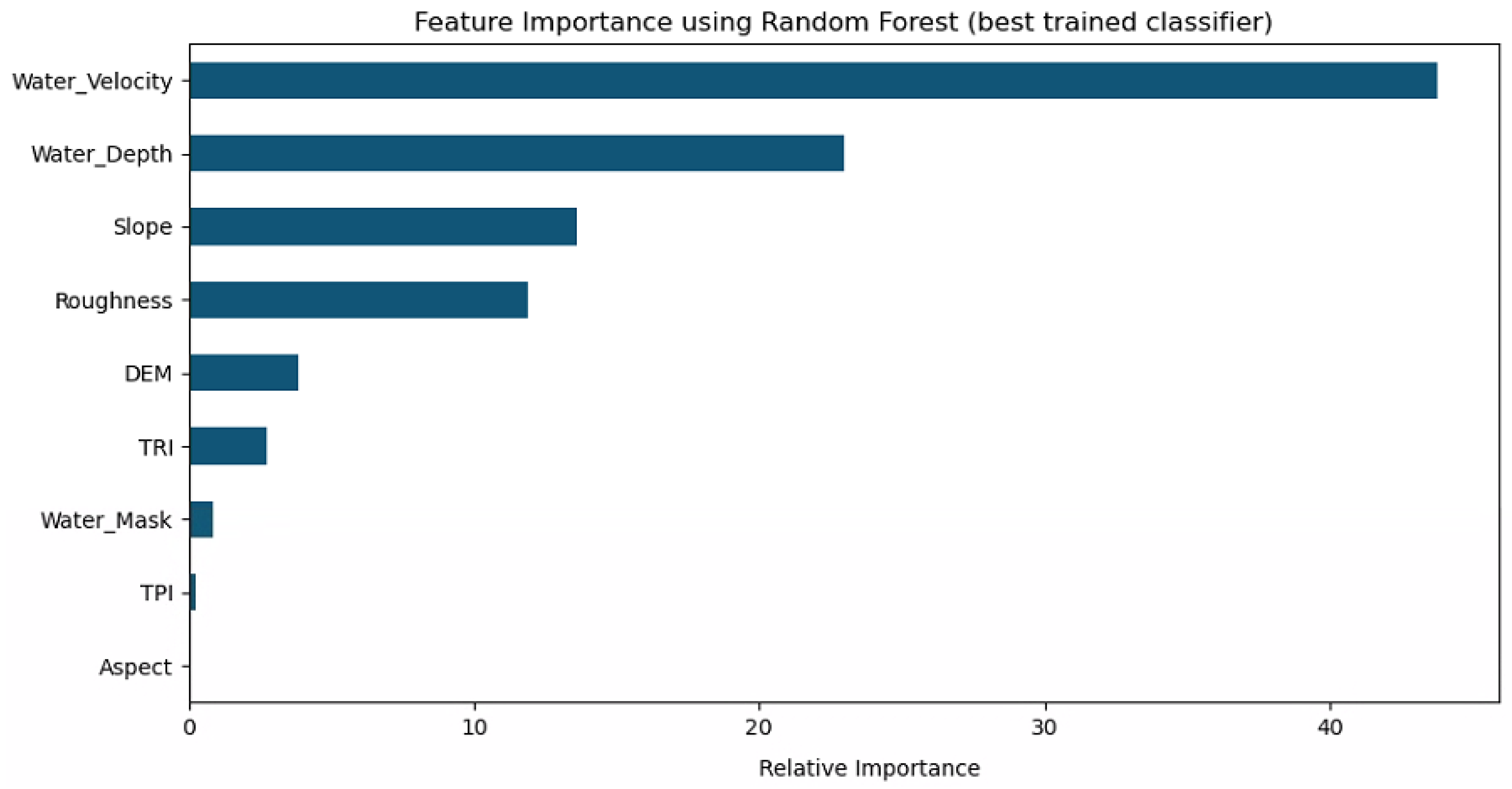
| Feature | Relative Importance Score |
|---|---|
| Water Velocity | 43.75939 |
| Water Depth | 22.99143 |
| Slope | 13.60606 |
| Roughness | 11.90979 |
| DEM | 3.87064 |
| TRI | 2.73504 |
| TPI | 0.23988 |
| Water Mask | 0.84437 |
| Aspect | 0.04339 |
Publisher’s Note: MDPI stays neutral with regard to jurisdictional claims in published maps and institutional affiliations. |
© 2022 by the authors. Licensee MDPI, Basel, Switzerland. This article is an open access article distributed under the terms and conditions of the Creative Commons Attribution (CC BY) license (https://creativecommons.org/licenses/by/4.0/).
Share and Cite
Antzoulatos, G.; Kouloglou, I.-O.; Bakratsas, M.; Moumtzidou, A.; Gialampoukidis, I.; Karakostas, A.; Lombardo, F.; Fiorin, R.; Norbiato, D.; Ferri, M.; et al. Flood Hazard and Risk Mapping by Applying an Explainable Machine Learning Framework Using Satellite Imagery and GIS Data. Sustainability 2022, 14, 3251. https://doi.org/10.3390/su14063251
Antzoulatos G, Kouloglou I-O, Bakratsas M, Moumtzidou A, Gialampoukidis I, Karakostas A, Lombardo F, Fiorin R, Norbiato D, Ferri M, et al. Flood Hazard and Risk Mapping by Applying an Explainable Machine Learning Framework Using Satellite Imagery and GIS Data. Sustainability. 2022; 14(6):3251. https://doi.org/10.3390/su14063251
Chicago/Turabian StyleAntzoulatos, Gerasimos, Ioannis-Omiros Kouloglou, Marios Bakratsas, Anastasia Moumtzidou, Ilias Gialampoukidis, Anastasios Karakostas, Francesca Lombardo, Roberto Fiorin, Daniele Norbiato, Michele Ferri, and et al. 2022. "Flood Hazard and Risk Mapping by Applying an Explainable Machine Learning Framework Using Satellite Imagery and GIS Data" Sustainability 14, no. 6: 3251. https://doi.org/10.3390/su14063251
APA StyleAntzoulatos, G., Kouloglou, I.-O., Bakratsas, M., Moumtzidou, A., Gialampoukidis, I., Karakostas, A., Lombardo, F., Fiorin, R., Norbiato, D., Ferri, M., Symeonidis, A., Vrochidis, S., & Kompatsiaris, I. (2022). Flood Hazard and Risk Mapping by Applying an Explainable Machine Learning Framework Using Satellite Imagery and GIS Data. Sustainability, 14(6), 3251. https://doi.org/10.3390/su14063251