Response Surface Method to Calculate Energy Savings Associated with Thermal Comfort Improvement in Buildings

Abstract

In developed countries, a large part of the building stock in 2050 will consist of currently existing buildings. Consequently, in order to achieve the objectives in terms of energy efficiency in the building sector we must consider not only new infrastructures but also the old ones. A reduction in energy consumption for climate control of between 50 and 90% can be achieved by rehabilitation and the implementation of different energy efficiency measures. Currently, these measures to reduce energy consumption and associated CO₂ emissions can be modelled using computer tools. However, high precision and detail of thermal behaviour models through simulations can mean a great computational cost for companies, which results in a blockage of servers and workers. In this paper, the Response Surface Methodology (RSM) is presented as an innovative methodology for the simplification of models for calculation of the energy savings associated with thermal comfort improvement in buildings. A single-family house model, located in three different climates, is presented as a case study in order to validate the proposed methodology. Different scenarios were simulated, addressing heating and cooling temperature set points and external wall insulation represented by the transmittance (U-value). Results obtained from energy simulation using Design Builder were contrasted against those estimated from the simplified model extracted from the RSM analysis. The results revealed a deviation lower than 3% when comparing both methods. Therefore, the simplified mathematical prediction models are demonstrated to be suitable for the study of the energy performance of buildings, saving computational time, costs and associated human resources.

1. Introduction

The European Union aims at becoming the first climate-neutral continent in the world by 2050 [1]. The building sector is one of the main producers of greenhouse gas emissions, so it should be a key actor in the decarbonisation strategy [2]. Rising living standards and demand for new energy services are putting upward pressure on energy demand in the sector. In the EU, this sector represents approximately 40% of the total final energy consumption [3] and the associated CO₂ emissions. In addition, this percentage is expected to grow due to the increase in cooling needs with the rise of the global temperature due to global warming [4]. The increase in Nearly Zero Energy Buildings (nZEB) is contemplated in the EU Directive 2010/31/EU [5] as an objective to improve the energy efficiency in buildings and thus reduce CO₂ emissions in the EU Member States. This directive was amended by Directive 2018/844/EU [6] with the aim of modernizing the building sector and increasing building renovations. In particular, the renovation wave strategy, presented within the European Green Deal [7], sets up a plan towards doubling the building renovation rate by 2030.

There is a consolidated market for existing buildings, although it remains to be assumed that this building stock meets current requirements in terms of health, comfort and energy performance [8]. In-depth building refurbishment is a key mitigation strategy in countries with a large number of available dwellings. This type of rehabilitation can have a very considerable impact on improving global energy efficiency, to the extent that the existing building stock is very numerous. For this reason, the energy refurbishment of existing buildings is contemplated, in the recent European directives, as a means to reduce energy consumption in them. The Energy Efficiency Plan of the European Commission (EC) has defined its objectives for the period from 2021 to 2030 as: (1) Reduction of 40% in the emission of greenhouse gases compared to levels of 1990, (2) contribution of 32% to the final energy consumption of renewable energies and (3) reduction of 32.5% in the consumption of primary energy (measures of saving and energy efficiency). These objectives are indispensable for the fulfilment of the commitments accepted in the Kyoto Protocol and the subsequent Paris agreement (signed in 2016 [9]), within the framework of the United Nations Framework Convention on Climate Change (UNFCCC). In order to achieve these objectives, the different Member States have set a roadmap following the guidelines of the European Directive. These new policies in the building sector may enable global energy consumption in buildings to stabilize or even decrease by the mid-21st century. However, the long life of buildings carries a risk of stagnation in the reduction in energy consumption in the building sector. Unlike the production of consumer goods, the production of buildings already incorporates the concept of durability (there is no such thing as “programmed obsolescence”). In this context, current new technologies lead to a new dynamic of greater efficiency in the productivity of the construction industry, which makes the simulation of the building’s energy performance an extremely interesting option to consider [10,11]. Simulations are very useful during the building design phase as they allow the prediction of energy demand or consumption values, facilitating the comparison of different scenarios with the inclusion of a series of energy efficiency measures in the design phase of the refurbishment. Energy simulations and accurate energy performance forecasting are also very valuable for the provision of advanced energy services based on the continuous metering and parameter data collection and ingestion through Building Information Modelling (BIM). These services may range from smart retrofitting, implicit and explicit energy efficiency and self-consumption optimization conducted by Energy Service Companies (ESCo) to demand response services delivered by demand side aggregators to grid operators.

1.1. Building Energy Performance Simulation Catalogue at Present

The number of simulation tools oriented to obtain the energy demand of a building are quite numerous [12]. These tools are called by their acronym BEPS (Building Energy Performance Simulation) and allow rigorous analysis that will be used in the decision-making process by energy service providers and building managers within acceptable risk levels [13]. Since the 1960s, hundreds of programs have been developed by both researchers and engineers. Some authors present a comparison of the most employed BEPS [14,15]. Among the programs studied are: BLAST, DOE-2, EnergyPlus, ESP-r or TRNSYS, which are the most used ones. However, the use of BIM tools is still rare in the field of energy efficiency, and even more so when it comes to modelling the renovation of existing buildings. In recent years, these tools have proven to have great potential for efficient energy management and optimization [16,17] due to the increasing demand for the use of this type of modelling as a mandatory tool for official projects in several developed countries [18]. In addition, the facilitated energy management and the subsequent life cycle analysis (LCA), where savings related to CO₂ emissions to the atmosphere, are also taken into account [19]. All these tools can be used for the evaluation of the thermal demand under certain conditions and for the estimation of the savings of energy consumption and associated emissions that are expected to be achieved after the implementation of different measures of energy efficiency and constructive solutions in a modelling environment. It is important to note that an energy model is not an accurate reflection of reality, and therefore simulations can present large discrepancies with the true behaviour of the system they represent. This is because, unlike physical experiments, computer experiments are performed on the basis of simplifications of reality [20,21]. However, they offer a great advantage since they are responses generated from predefined stochastic algorithms [22]. Nonetheless, these tools imply a great effort (time, cost and human resources) to carry out simulations for different scenarios.

Of all the existing BEPS, EnergyPlus is the most used to perform the analysis with respect to the dynamic thermal simulations, using Design Builder as the graphic interface. EnergyPlus calculates loads by means of heat balance, which are then used in the system simulation module where the response of the heating and cooling systems is calculated. Through the integrated simulation, a more accurate prediction of the interior temperature is achieved. DesignBuilder software (DB, Design builder software. http://www.designbuilder.co.uk, accessed on 10 January 2022) is developed on the input requirements of EnergyPlus (calculation engine), which is the U.S. DoE (U.S. Department of Energy) building energy simulation program for the modelling and calculation of heating, cooling, lighting, ventilation and other energy flows. This software is one of the most advanced building energy simulation tools in the market, which simplifies the modelling process and the analysis of the results. For this reason, Design Builder has been chosen for the development of this study, however, if the proposed hypotheses are met, this methodology could be used for any other energy simulation software.

1.2. Response Surface Methodology as an Alternative Method

The Response Surface Methodology (RSM) is a mathematical and statistical technique that allows the study of the effect produced by independent variables on another dependent variable or response. RSM models and optimizes a process by using several variables which affect the model response [23]. Central Composite Design (CCD) is the most employed RSM design that can decrease the number of experiments and equally predict the possible non-linear effect of each parameter and the possible interactions between them. RSM has been successfully used in several research fields through the application of CCD. The areas where it has been applied are diverse, in engineering fields such as the synthesis of oxygen in nanocomponents, study of the effects of low-frequency oscillations in the generation of energy by wind generators, or even the elimination of iron components in binary mixtures of dyes [24,25,26], structural fields, where Response Surface Models have been used in the study of the quality of welds in metal structures, predicting parameters such as the tensile strength, impact toughness and hardness of friction [27,28]; in construction, this methodology has been used in the study of mixtures’ optimization for mortar and concrete, analysing properties required by EN regulations for these materials [29,30,31], among others. Within the field of energy, application studies have been found in the optimization of energy processes and fuel consumption or BTE and NOx Optimization using ANOVA analysis [32,33].

Although research using other statistical and calibration methods have been conducted [34], BESF models themselves use different methodologies to simplify their simulations, such as screening [35], analysis of variance [36,37] or metamodeling (BACCO) [38].

In this paper, Response Surface Methodology, combined with energy simulation tools, is presented as an innovative methodology for the calculation of the energy savings associated with the thermal comfort improvement in all types of buildings, reducing the need for complex simulations. The proposed methodology allows studying trend scenarios under controlled conditions, obtaining a simple model that gives a quick response. This simple model is developed to work within the established ranges without the need to use complex simulation tools, achieving a quick response and flexible to different variables, saving calculation time, costs and associated human resources.

2. Methodology and Case Study

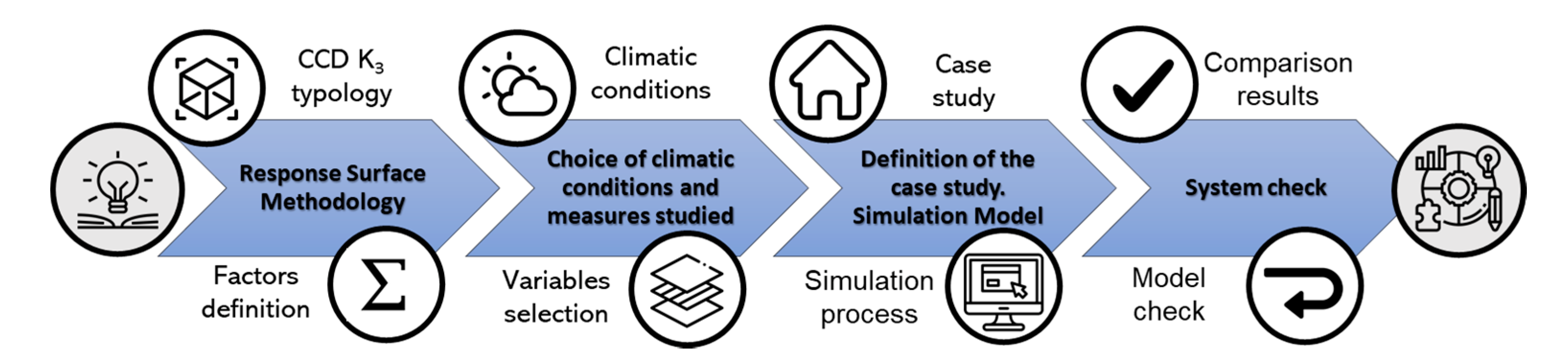
This section presents the methodology followed for the verification of the Response Surface Method as a simplification element in energy simulations using EnergyPlus. Firstly, the theoretical foundations governing the calculations using RSM are described. Subsequently, the particularities of the case study used for such verification and implemented with the Showare Design Building v4 are presented and an explanation is given of the measures studied and the reasons for their choice.

This experimental program (Figure 1) is divided into four phases: (1) Response Surface Methodology, (2) choice of climatic conditions and measures studied, (3) definition of the case study and simulation model and (4) system check.

2.1. Response Surface Methodology

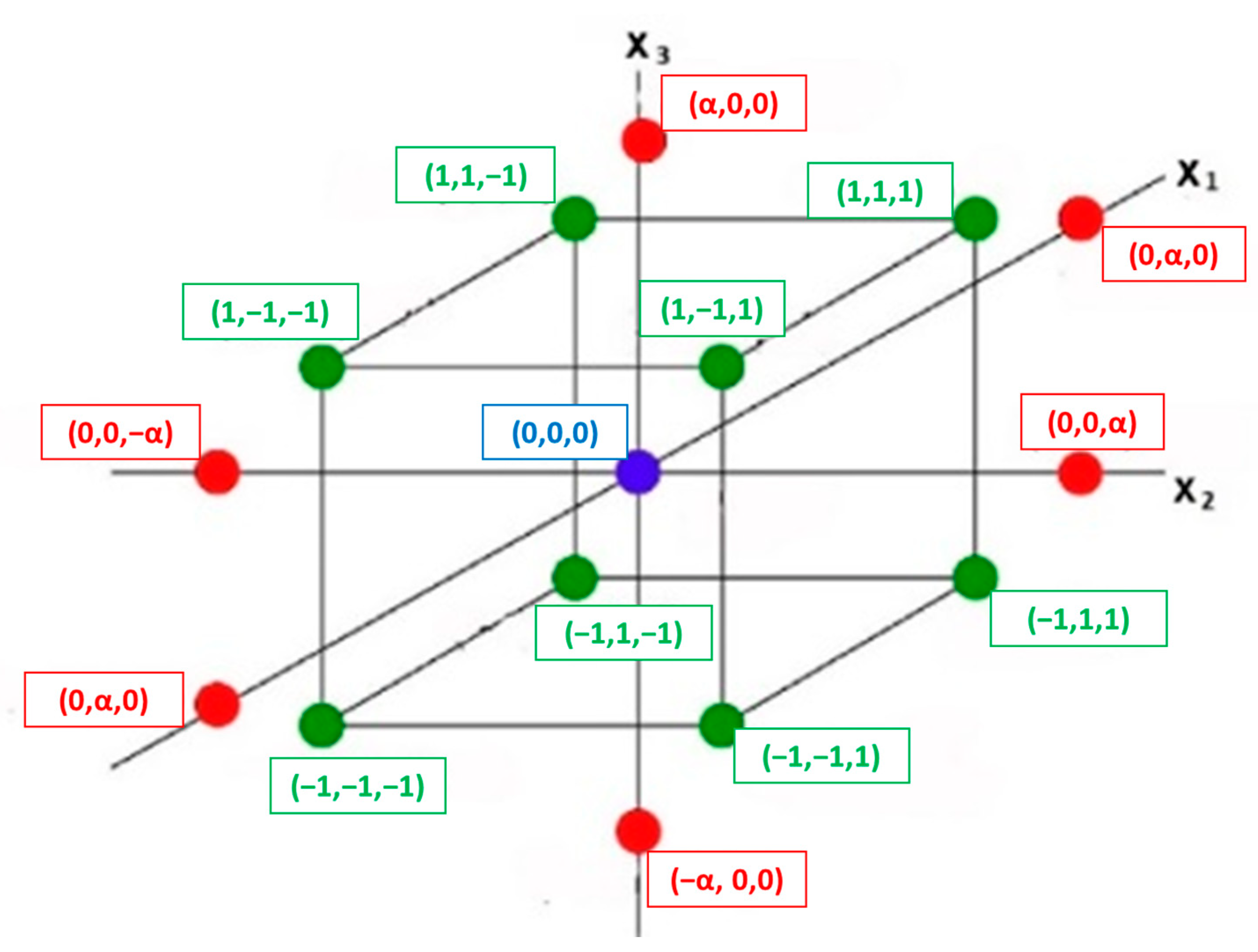
Next, the Response Surface Method (RSM) is applied with the Central Composite Design to verify the data obtained in the different simulations. Minitab uses CCD K₃ typology, where the main characteristics are:

• Use of three factors,
• Matrix of experiments with three levels for each factor, as shown in Figure 2.

• Coding of the ranges of values of the three factors to varying between (−1, 1) (

  Table 1. Variable range of studio and coded.

  Variables	Range		Coded Variables* [x1*, x2*, x3*] [HT*, CT*, I*]
  			−1	−0.5 1	0	0.5 1	1
  (x1) = (HT) Heating set point (°C)	20	28	20	22	24	26	28
  (x2) = (CT) Cooling set point (°C)	22	30	22	24	26	28	30
  (x3) = (TW) U-value (W/m2-K)	1.3	0.1	1.3	1.0	0.7	0.4	0.1

  ¹ Used for the system check.

  ), according to Equation (2).
• Use of a quadratic module defined in Equation (1), for the adjustment of the response surface of each regression factor.
• The response surface will allow the estimation of the behaviour of any coded point within the cube defined by the ends.

Actual parameter values must be pre-coded. Minitab uses coded configuration values for the factors, which are presented below:

• −1: indicates low level of the factor,
• 0: indicates the intermediate point between low level and the highest level,
• 1: indicates high level of the factor,
• α: indicates, in codified units, the location of the axial points in the design.

These parameters, x₁, x₂ and x₃, are the ones that will govern the response surface. The relationship between these parameters and the response surface can be expressed as ƒ (x₁*, x₂*, x₃*), where ƒ is postulated as a quadratic model where x₁*, x₂* and x₃* are the coded variables x₁, x₂ and x₃, respectively. The incorporation of the axial design value (α) is not considered because unreasonable values would be required for this research, so the values -α and α have been replaced by the values −1 and 1, respectively.

ƒ (x₁*, x₂*, x₃*) = b₀ + b₁ × x₁* + b₂ × x₂* + b₃ × x₃* + b₁₁ × x₁*² + b₂₂ × x₂*² + b₃₃ × x₃*² + b₁₂ × x₁* × x₂* + b₁₃ × x₁* × x₃* + b₂₃ × x₂* × x₃*

(1)

For any real value X_i of the variable parameters, this coding can be completed through the expression (Equation (2)), obtaining the corresponding coded value x_i. Where X_iNInf is the real value of the lowest level of the i-factor, X_iNSup is the real value of the highest level of the i-factor and Ẍi is the measurement between the real values of the highest and lowest level of the i-factor = (x₁*, x₂*, x₃*).

$$x_i=\frac{2\times 1\left(X_i-{{Ẍ}}_i\right)}{X_{iNSup}-X_{iNInf}}$$

(2)

Values are saved with the help of a statistical software that contains the RSM function; in this paper, Minitab^® 19 (Stat Soft Inc., Tulsa, Tulsa, OK, USA) (Minitab. https://www.minitab.com/es-mx/, accessed on 10 January 2022) is used, then, the regression coefficients (b₀, b₁, b₂, b₃, b₁₁, b₂₂, b₃₃, b₁₂, b₁₃ y b₂₃) of the function ƒ (x₁*, x₂*, x₃*) are determined. With these coefficients, it is possible to estimate the value of the response for any combination of the values of parameters (x₁*, x₂*, x₃*) if these values are within the quadratic domain defined previously for this design. Response surface graphs are used for the representation of ƒ (x₁*, x₂*, x₃*), where the blocking of one of the three parameters (e.g., x₁) is sufficient to represent the response as a function of the other two, e.g., x₂ and x₃.

Therefore, ƒ (x₁*, x₂*, x₃*) (Equation (1)) can be expressed as (HT*, CT*, TW*) (Equation (3)), where ƒ is postulated as a quadratic model where HT*, CT* and TW* are the coded variables of HT, CT and TW, respectively, following the indications in Table 1.

ƒ (HT*, CT*, TW*) = b₀ + b₁ × HT* + b₂ × CT* + b₃ × TW* + b₁₁ × HT*² + b₂₂ × CT*² + b₃₃ × TW*² + b₁₂ × HT* × CT* + b₁₃ × HT* × TW* + b₂₃ × CT* × TW*

(3)

2.2. Choice of Climatic Conditions and Measures Studied

Three cities have been chosen for the study of different representative climatic zones of Europe, according to Köppen [39]: Madrid (Csa—Typical Mediterranean), Paris (Cfb—Temperate ocean) and Warsaw (Dfb—Hemi-boreal without dry season). The climatic conditions of the three places are shown in

Table 2. Weather conditions.

City	Weather	Average Annual Temperature	Rainfall Annual
Madrid	Csa—Mediterranean hot summer climate	13.8 °C	437 mm
Paris	Cfb—Oceanic climate	11.3 °C	637 mm
Warsaw	Dfb—Hemi-boreal climate	7.7 °C	201 mm

(Climate Data. https://es.climate-data.org/ accessed on 10 January 2022).

In this paper, total energy demand (obtained as the sum of heating demand and cooling demand) is the dependent variable or response studied. Independent variables used are the set point temperature for the heating system (HT), the set point temperature for the cooling system (CT) and U-value of exterior walls (TW). The selected variables and their study ranges are representative of the analysis of energy-saving measures.

Thermal control systems (thermostats and systems that allow adjusting consumption to thermal needs and adapting them to the outside temperature) allow a reduction of between 10% and 30% [40] in heating and cooling consumption. The low cost and rapid return on investment of these actions give rise to a high potential for their large-scale adaptation in the coming years. Likewise, the ease of installation and the great energy savings make the investments in the rest of the actions more efficient. The temperature variation considered corresponds to the comfort zones for the winter season (20–24 °C) and the summer season (24–28 °C). These ranges are extended in this research (20–28 °C) and (22–30 °C), respectively, to have a wider analysis. The ideal temperatures of 21 °C and 26 °C, respectively, are within these variable ranges.

On the other hand, approximately 75% of a building’s energy losses occur through the building envelope (windows, facades, roof and floor). Therefore, the quality of the exterior walls is one of the factors that most improves the energy performance of buildings. Similarly, the rehabilitation of facades to increase thermal insulation has great potential for savings (between 30 and 60% compared to buildings constructed before 1980) [41]. However, this action requires a high initial investment and a longer payback period. The variation U-value is studied from 1.3 W/m²-K cm for exterior walls to 0.1 W/m²-K, which is common in countries with a cold climate.

CCD provides 15 combinations per experiment. In this study, three different types of experiments were conducted according to the type of climate of each city: Madrid (first experiment), Paris (second experiment) and Warsaw (third experiment).

2.3. Definition of the Case Study and Simulation Model

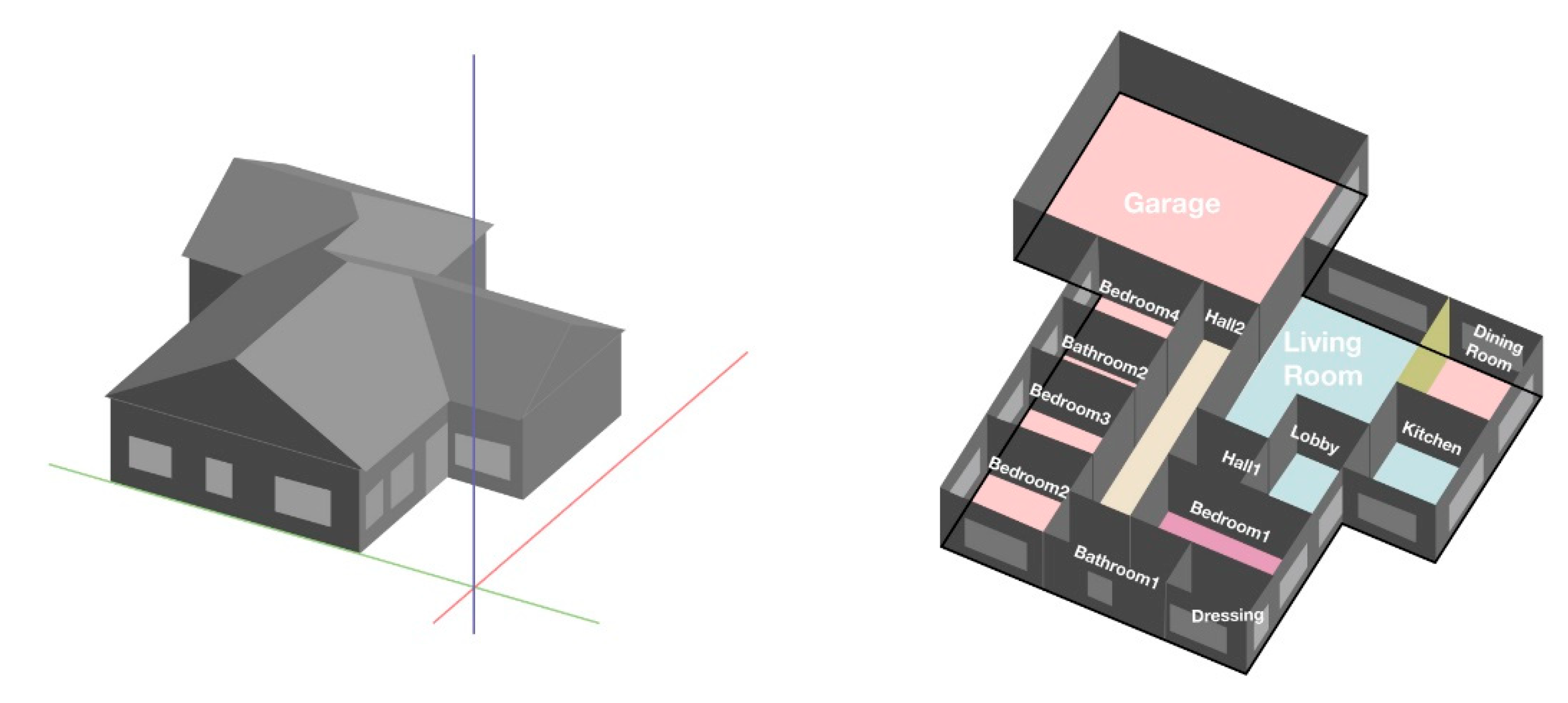
Firstly, from the constructive design of the building, energy simulations are carried out to establish the basic energy consumption of the building. The methodology developed is a single-family house (Figure 3), whose construction characteristics are specified in

Table 3. Main characteristic of case study.

Main Characteristic of Case Study
Surface (m2)	124
Height (m)	3.5
Regular occupants	0.05 person/m2
UOpaque envelope (W/m2-K)	External wall: Variable Roof: 2.930 Basement floor: 0.25
Infiltrations (air changing per hour)	0.70
Uwindows (W/m2-K)	Glass 1.924 Frame 3.633
WWR (N%; S%; W%; E%)	14.12%; 14.95%; 13.57%; 13.90%
Cooling system	Electrical Central Chiller
Cooling system efficiency	COP = 1.8
Heating system	Natural gas boiler
Heating efficiency	COP = 0.85
Ventilation type	Only Local Extract (single duct)

.

Likewise, in the definition phase, a series of concepts related to the use of the building have been estimated. The thermal behaviour of a building is influenced, to varying degrees, by a series of factors that must be defined in the simulation, based on the levels of occupation, schedules, behavioural patterns and habitability of the users or equipment. In the case of residential buildings, some of these concepts do not represent a great influence to be considered in the calculation of energy demand, however, there are other concepts that have a greater impact, such as configuration, location, orientation or the presence of external shadows, construction characteristics, external environmental conditions and internal conditions such as temperature, relative humidity or degree of ventilation.

2.4. System Check

Finally, the verification of both methodologies is carried out with the comparison of the data obtained between them. To test the methodology, 125 combinations inside the study ranges have been analysed to verify whether the values obtained by both methods are equivalent. Firstly, the points proposed in the RSM method have been compared (15 points) and the remaining combinations resulting from the three ranges of the three variables were then compared (+14 points). Then, to ensure that the method works within the proposed cube, the resulting combinations of the intermediate points belonging to the code −0.5 and 0.5 (see Table 1) and the combinations of these points with those previously coded have been analysed (+96 points). In order to carry out all test simulations to use jEPlus software (jEPlus–An EnergyPlus simulation manager for parametrics. www.jeplus.org, accessed on 10 January 2022) is possible, which is developed to resolve parametric simulations that act as a black box including its inputs, outputs and parameters. Using this software, it is possible to automate the simulation process, saving human resources both in the process of obtaining the design of experiments (in the case of very extended simulations in time) and, also, in the process of checking whether it is necessary.

3. Results and Discussion

In this section, the results obtained from each of the experiments with the energy simulation method and the statistical method are analysed in detail. Values were obtained after the energy simulation of our building (characteristics shown in Table 2). This energy demand (along with the simulation energy demand and the heating energy demand) is shown in Table 5.

Once the coded variables (Table 1) have been processed by Minitab^® statistical software, the regression coefficients obtained in the calculation of RSM are shown in

Table 4. Regression coefficients for experiments.

Experiment 1: Madrid
	β0	β1	β2	β3	β11	β22	Β33	β12	β13	β23	R2 (%)
Regression coefficients	15,257.9	5112.3	−2305.4	−3581.7	519.9	316.2	−586.8	0.0	−1275.7	326.8	99.97
Valor p	0.000	0.000	0.000	0.000	0.003	0.021	0.002	1.000	0.000	0.002
FIV		1.00	1.00	1.00	1.30	1.30	1.30	1.00	1.00	1.00
Experiment 2: Paris
	β0	β1	β2	β3	β11	β22	Β33	β12	β13	β23	R2 (%)
Regression coefficients	19,162.0	6169.8	−1592.1	−4575.2	300.2	533.4	−685.9	0.0	−1379.6	58.2	99.98
Valor p	0.000	0.000	0.000	0.000	0.025	0.003	0.001	1.000	0.000	0.331
FIV		1.00	1.00	1.00	1.30	1.30	1.30	1.00	1.00	1.00
Experiment 3: Warsaw
	β0	β1	β2	β3	β11	β22	Β33	β12	β13	β23	R2 (%)
Regression coefficients	24,045.5	6310.2	−1175.5	−5808.4	272.2	473.9	−848.1	0.0	−1344.0	−23.2	99.98
Valor p	0.000	0.000	0.000	0.000	0.0039	0.005	0.000	1.000	0.000	0.0693
FIV	1.00	1.00	1.00	1.30	1.30	1.30	1.00	1.00	1.00	1.00

. The study has been carried out only with the total energy demand, understanding that this shows the behaviour of both cooling and heating.

Statistically, the regression is significant and explains more than 99.5% of the variance for all cases. It can be assumed that the coefficient β₁₂ is not significant (shown with an artery). However, as stated in other studies [42], the non-significant coefficients help to contribute to the proper shape of the response surface, so it is not advisable to remove them from ƒ (HT*, CT*, TW*). Total Demand response surfaces obtained from the coefficients in Table 4 are represented by the following equations (Equations (4)–(6)).

ƒ_{(Total demand − Madrid)} (HT*, CT*, TW*) = 15,257.9 + 5112.3 × HT* − 2305.4 × CT* − 3581.7 × TW* + 519.9 × HT*² + 316.2 × CT*² − 586.8 × TW*² − 1275.7 × HT* × TW* + 326.8 × CT* × TW*

(4)

ƒ _{(Total demand − Paris)} (HT*, CT*, TW*) = 19,162.0 + 6169.8 × HT* − 1592.1 × CT* − 4575.2 × TW* + 300.2 × HT*² + 533.4 × CT*² − 685.9 × TW*² − 1379.6 × HT* × TW* + 58.2 × CT* × TW*

(5)

ƒ _{(Total demand − Warsaw)} (HT*, CT*, TW*) = 24,045.5 + 6310.2 × HT* − 1176.6 × CT* − 5808.4 × TW* + 272.2 × HT*² + 473.9 × CT*² − 848.1 × TW*² − 1344.0 × HT* × TW* − 23.2 × CT* × TW*

(6)

Thus,

Table 5. Simulated (Design Builder) energy demand and test results using RSM.

		Experiment 1 (Madrid)				Experiment 2 (Paris)				Experiment 3 (Warsaw)
		Heating Demand (kWh)	Cooling Demand (kWh)	Total Demand (kWh)		Heating Demand (kWh)	Cooling Demand (kWh)	Total Demand (kWh)		Heating Demand (kWh)	Cooling Demand (kWh)	Total Demand (kWh)
				DB	RSM			DB	RSM			DB	RSM
1	(−1,−1,−1)	7679.73	7706.48	15,386.21	15,333.02	13,979.93	4067.45	18,047.38	17,985.69	20,535.14	2782.23	23,317.37	23,251.11
2	(1,−1,−1)	20,370.81	7706.48	28,077.29	28,109.00	28,984.99	4067.45	33,052.44	33,084.56	35,738.63	2782.23	38,520.86	38,559.32
3	(−1,1,−1)	7679.73	2475.86	10,155.59	10,068.63	13,979.93	786.28	14,766.21	14,685.19	20,535.14	483.79	21,018.93	20,944.56
4	(1,1,−1)	20,370.81	2475.86	22,846.67	22,844.61	28,984.99	786.28	29,771.27	29,784.06	35,738.63	483.79	36,222.42	36,252.78
5	(−1,−1,1)	3580.83	6483.44	10,064.27	10,067.47	7329.97	4159.87	11,489.84	11,478.17	11,248.59	3149.89	14,398.48	14,368.64
6	(1,−1,1)	11,169.29	6483.44	17,652.73	17,740.83	16,816.6	4159.87	20,976.47	21,058.61	21,076.27	3149.89	24,226.16	24,301.05
7	(−1,1,1)	3580.83	2559.89	6140.72	6110.15	7329.97	1111.42	8441.39	8410.40	11,248.59	758.47	12,007.06	11,969.12
8	(1,1,1)	11,169.29	2559.89	13,729.18	13,783.51	16,816.60	1111.42	17,928.02	17,990.84	21,076.27	758.47	21,834.74	21,901.52
9	(−1,0,0)	5895.56	4602.38	10,497.94	10,665.46	11,100.67	2006.28	13,106.95	13,292.32	16,500.61	1298.54	17,799.15	18,007.55
10	(1,0,0)	16,459.84	4602.38	21,062.22	20,890.14	23,815.56	2006.28	25,821.84	25,631.98	29,539.82	1298.54	30,838.36	30,627.86
11	(0,−1,0)	10,646.36	7302.91	17,949.27	17,879.45	17,146.73	4181.61	21,328.34	21,287.44	22,742.80	2970.44	25,713.24	25,695.98
12	(0,1,0)	10,646.36	2556.98	13,203.34	13,268.60	17,146.73	920.17	18,066.90	18,103.31	22,742.80	584.98	23,327.78	23,342.95
13	(0,0,−1)	13,456.74	4685.45	18,142.19	18,252.70	21,139.03	1814.48	22,953.51	23,051.32	27,795.10	1138.90	28,934.00	29,005.81
14	(0,0,1)	6909.18	4295.27	11,204.45	11,089.38	11,776.53	2226.72	14,003.25	13,900.95	15,927.45	1535.40	17,462.85	17,388.95
15	(0,0,0)	10,646.36	4602.38	15,248.74	15,257.86	17,146.73	2006.28	19,153.01	19,161.99	22,742.80	1298.54	24,041.34	24,045.52

shows the results obtained in the simulations carried out by Design Builder (DB) and the response values estimated by the response surface model (RSM) for the different combinations.

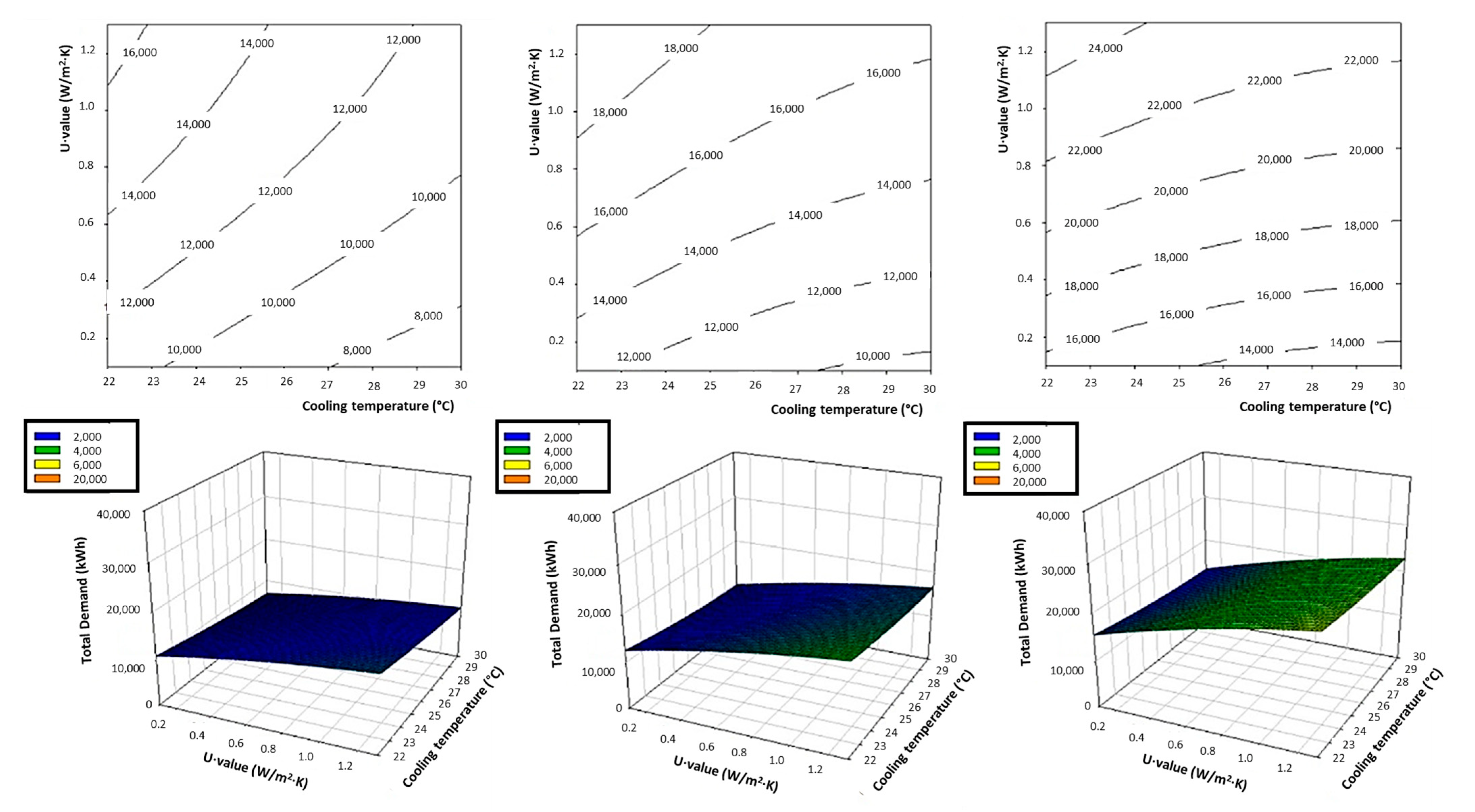
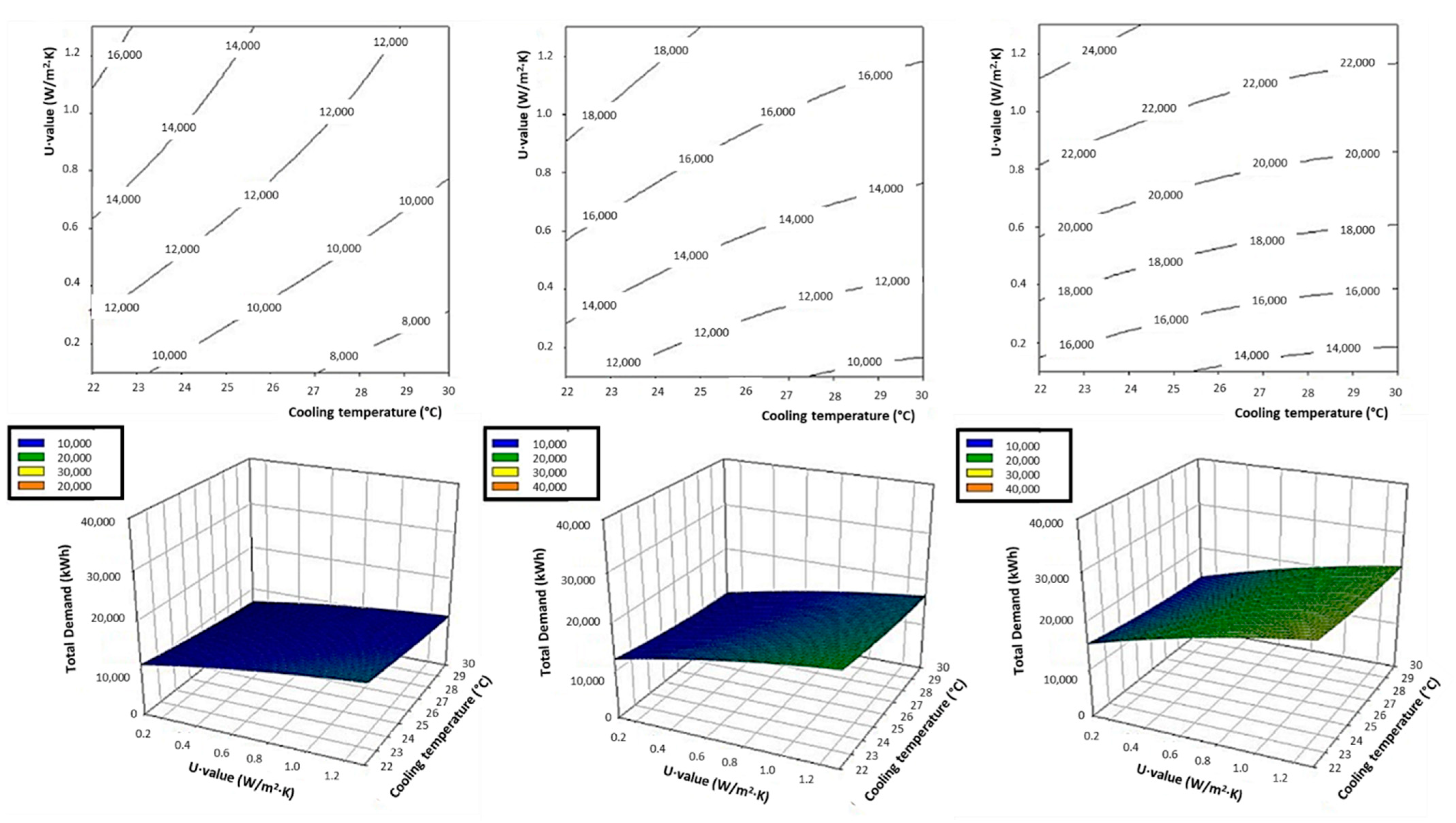
The 2D and 3D graphic representation of the response surface equation is used for this purpose (Figure 4, Figure 5 and Figure 6). In the first and second place, the heating temperature set point is fixed at 21 °C and the cooling temperature set point is fixed at 26 °C; both temperatures are coincident with the ideal comfort temperatures. Thirdly, the fixed U-value will be 1.22 W/m²-K (maximum U-value allowed by CTE) [43].

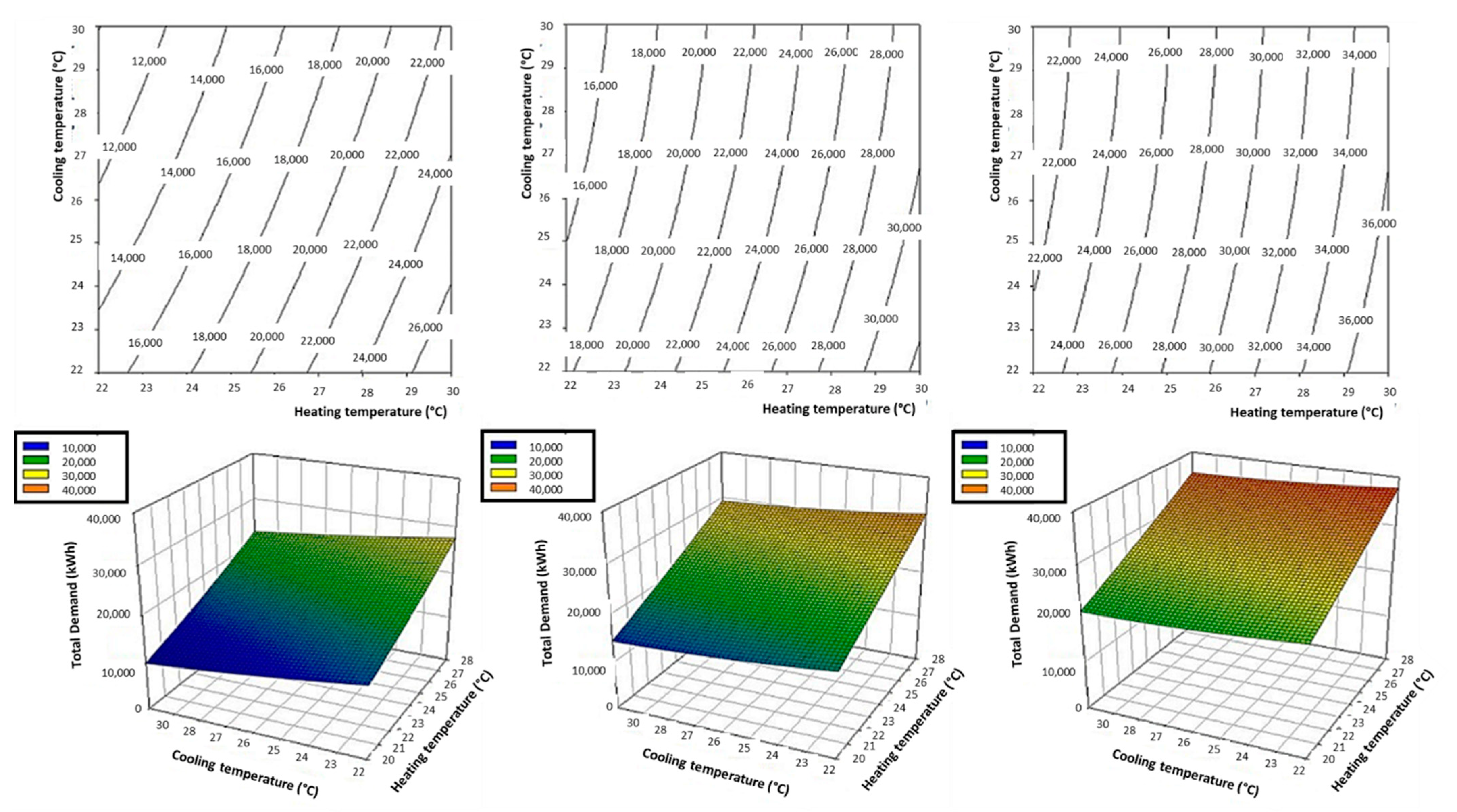
The heating and cooling demands for the three climate zones can be evaluated. In all three climate zones, the heating demand carries more weight than the cooling demand, although, as expected, the relative proportion of these demands in construction is different in each climate zone and is higher in the more extreme European climates. The greatest demand for heating is observed in the city of Warsaw, due to its climate (Hemi-boreal without dry season) which gives it very low temperatures in winter. In addition, this city has few hours of sunshine in the winter season, which makes its residents spend more hours in their homes and thus increases the demand for heating. On the other hand, the low influence of the cooling system on the total demand for air conditioning is explained by the fact that only the climate of Madrid (Typical Mediterranean) can be considered warm, and therefore this system is necessary. In the case of Paris and Warsaw, the lack of thermal comfort during the summer is not sufficient for the common population to install cooling systems in their homes.

Considering the influence of the construction system and the increase in the thickness of the insulation, Figure 4 shows how good thermal insulation helps to cool spaces, however, the energy savings due to the cooling system are stabilised at very high insulation thicknesses. The cooling set point has not much influence on the energy demand, probably because there are not too many warm climates where the studied temperatures are often reached. Figure 5 shows the high energy demand required when raising the heating system’s set point because more energy is needed to reach higher temperatures. It also shows the large energy reduction caused by good thermal insulation of the building envelope. Finally, Figure 6 replicates and confirms the tendencies previously observed. For the same U-value, the heating set point’s influence is greater than the cooling set point. A greater inclination of the plane with respect to the heating axis than on the cooling axis is observed. Total thermal demand is higher for higher heating temperatures; while this varies little between temperatures, Madrid is the city with the greatest variation, because it is the hottest climate of the three.

Methodology Check

The data obtained and the analyses exposed above show how the predictions made by the Response Surface Method fit the values obtained by the simulations. In addition, the progressions sent by the method show a reliable adaptation to the reality of consumption expected in different situations. In order to guarantee an adequate, reliable and more accurate response, the data obtained are checked.

After carrying out the 15 simulations established in our design of experiments, a greater number of simulations have been carried out to compare the data obtained in them with the response provided by the quadratic models. The regression line has been obtained by comparing both values for each of the points. For the 15 combinations obtained as input for the design of experiments, an R² greater than 99%, as in the data provided by Minitab, has been obtained (Table 4). 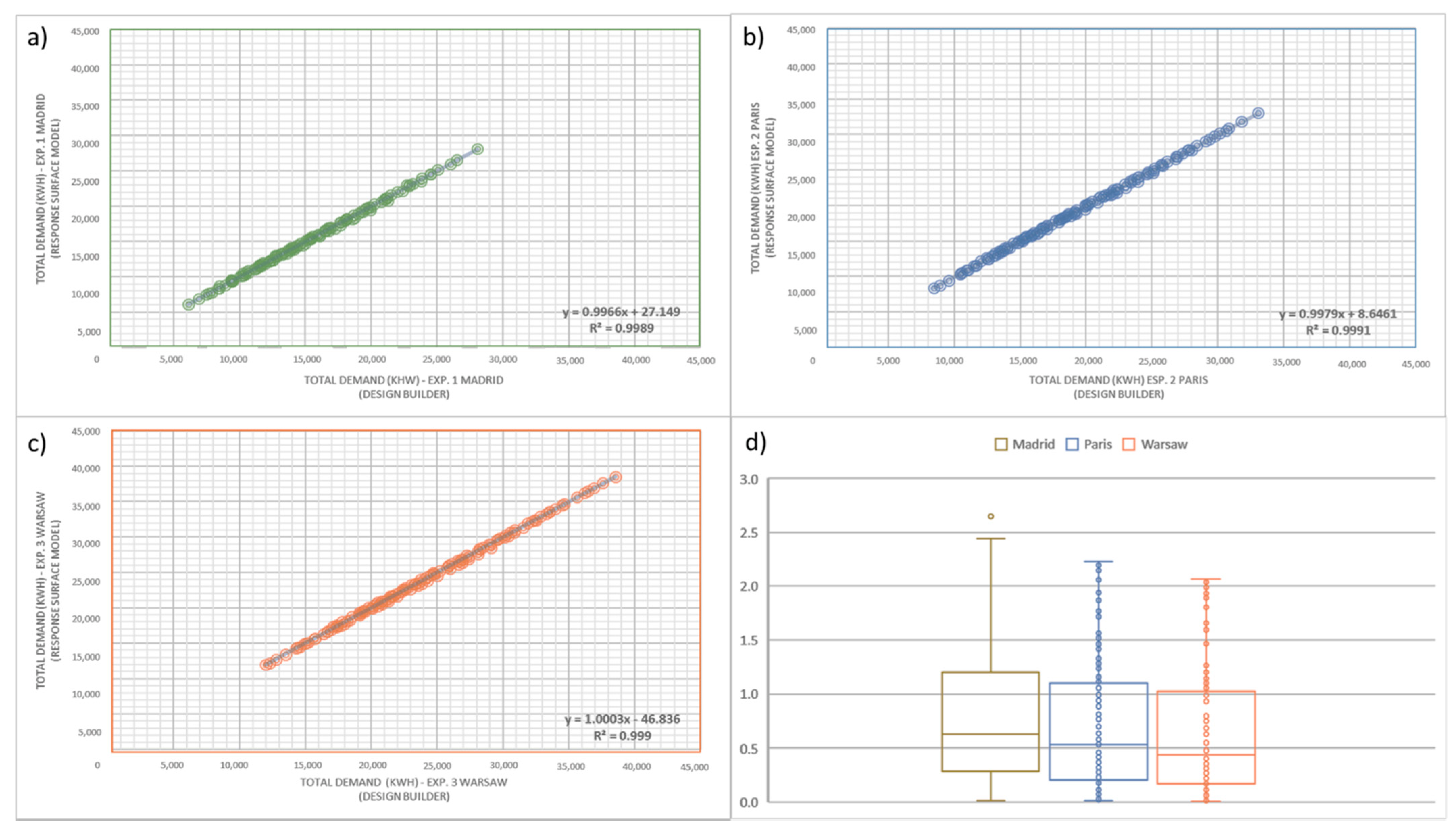Figure 7a–c shows the regression lines obtained for all the analysed combinations within the range studied in the three experiments and correlation coefficients. The fit of all the lines indicates that all the equations that define the response surfaces obtained are also representative at the interior points of the study.

Additionally, knowing that the results by both methods are not exact, since both predict behaviour in different ways, the percentage of error between both methods has been calculated (Figure 7d). The percentage of error between the simulated energy demand and the calculated energy demand shows the deviation between both methods. The average percentage difference between each pair of values is 0.83% for the first experiment, with a maximum of 2.65%, 0.71% with a maximum of 2.23% for the second experiment and 0.63% with a maximum of 2.07% for the third experiment. The maximum and average percentages obtained are low compared to those admissible in energy simulation processes, where percentages lower than 10% can be admitted. Therefore, after checking both methodologies, to use the design of experiments by means of RSM to know the demand of air conditioning of a building without the need to carry out the corresponding simulation is possible, and the good behaviour of the Response Surface Method in energy simulations can be guaranteed to reduce energy simulation costs. Since, after the similarity of the results, it is possible to reduce the number of simulations in our building (controlled environment) to the number of simulations required to feed the RSM, only a total of 15, using human capital and computational hours required only in this phase of the study. After carrying out this small number of simulations and creating the RSM, the energy behaviour of the building studied for any possible combination of the chosen parameters can be obtained by means of the RSM equation (almost instantaneous in time) without the need to enter the parameters in the simulation software and launch the new simulation (with the computational and time cost). In the same way, to know the behaviour of the energy demand, as shown in the examples of the Figure 4, Figure 5 and Figure 6, it would be necessary to carry out innumerable energy simulations using all the possible combinations of parameters and carrying out the extrapolation of results, an operation that seems unfeasible in resources. On the other hand, the study of this behaviour is easily achievable using the combination of both methods.

4. Conclusions

The deployment of new data-driven energy services in buildings requires advanced modelling and forecasting algorithms to enable the on-time provision of energy efficiency and demand response strategies and a suitable performance measurement and verification protocol. For this purpose, energy simulations and performance modelling are key in the novel energy services of the future. This requires heavy computing and management costs, and alternative methods must be explored.

The Response Surface Methodology applied to the study of energy demand in buildings is suitable for explaining the tendency scenarios of the building’s thermal behaviour. The response surfaces obtained, using the Composite Central Design, adjust with an error of less than 3% to the results obtained through energy simulations, so the mathematical method of analysis is suitable for predicting the behaviours of this type. Therefore, reducing the number of simulations between 50% and 70% is possible, which leads to important savings in terms of time and computational costs and human resources, optimizing research processes.

In this way, finding a calculation method (Response Surface Methodology) capable of adapting and replacing a large volume of energy simulations has also been possible, obtaining an algorithm (black box) that allows estimating of energy consumption in air conditioning and obtaining a large amount of data to save time in simulations. This leads to obtaining of the energy demand of a building in a faster and easier way (on a known model) that can support non-technical workers or customers when they need to decide by consensus without needing complex simulation tools.

Although this study is not able to reflect all possible alternatives, both for architecture and materials, important conclusions that are very useful for future research can be extracted. In this light, this methodology can be replicated to lighting control systems, in different locations and thermal zones, as well as in buildings monitored through SCADA. Similarly, this forecast method can be used for the delivery of data-driven energy services in buildings, with any other reference factor chosen. Similarly, the application can be extended to the creation of advanced energy monitoring and energy analytics interfacing with energy service providers and building residents. Among the possible future investigations, the calibration of this methodology using real monitored building data can be considered. Additionally, the testing of the methodology by increasing the number of dependent variables using CCD K₄, CCD K₅ or higher designs, the study of the energy demand, not only thermal but also lighting, and the creation of a valid interface can be interesting as future development areas. Finally, this methodology can be implemented in BIM models and data-driven energy management systems for ESCo and energy service providers, allowing for improvement in demand forecasts and performance measurement and verification towards the implementation of a new generation of ESCo energy services based on the Pay-for-Performance approach.

References

- Committing to Climate-Neutrality by 2050: Commission Proposes European Climate Law and Consults on the European Climate Pact. Available online: https://www.europarl.europa.eu/cmsdata/230214/EU_commitment%20to%20climate-neutrality_by_2050.pdf (accessed on 10 January 2022).
- Mulvaney, D. Green New Deal. In Solar Power: Innovation, Sustainability, and Environmental Justice; University of California Press: Berkeley, CA, USA, 2019; pp. 47–65. [Google Scholar] [CrossRef]
- Economidou, M.; Atanasiu, B.; Despret, C.; Maio, J.; Nolte, I.; Rapf, O. Europe’s Buildings Under the Microscope. A Country-by-Country Review of the Energy Performance of Buildings; Buildings Performance Institute Europe: Brussels, Belgium, 2011; pp. 35–36. [Google Scholar]
- Kozarcanin, S.; Hanna, R.; Staffell, I.; Gross, R.; Andresen, G.B. Impact of climate change on the cost-optimal mix of decentralised heat pump and gas boiler technologies in Europe. Energy Policy 2020, 140, 111386. [Google Scholar] [CrossRef] [Green Version]
- European Parliament; Council of the European Union. Directive 2010/31/EU of the European Parliament and of the Council of 19 May 2010 on the energy performance of buildings. Off. J. Eur. Union L 2010, 13–35. Available online: https://eur-lex.europa.eu/legal-content/EN/TXT/?uri=celex%3A32010L0031 (accessed on 10 January 2022).
- European Parliament; Council of the European Union. Directive (EU) 2018/844 of the European Parliament and of the Council. Off. J. Eur. Union 2018. Available online: https://eur-lex.europa.eu/legal-content/EN/TXT/?uri=uriserv%3AOJ.L_.2018.156.01.0075.01.ENG (accessed on 10 January 2022).
- Sikora, A. European Green Deal—Legal and financial challenges of the climate change. ERA Forum 2020, 21, 681–697. [Google Scholar] [CrossRef]
- Cuchí, A.; Sweatman, P. Una visión-país para el sector de la edificación en España. GBCe CONAMA 2011, 70. Available online: http://www.encuentrolocal.vsf.es/download/bancorecursos/libro_GTR_cast_postimprenta.pdf (accessed on 10 January 2022).
- Christoff, P. The promissory note: COP 21 and the Paris Climate Agreement. Env. Polit. 2016, 25, 765–787. [Google Scholar] [CrossRef]
- Herrando, M.; Cambra, D.; Navarro, M.; de la Cruz, L.; Millan, G.; Zabalza, I. Energy Performance Certification of Faculty Buildings in Spain: The gap between estimated and real energy consumption. Energy Convers. Manag. 2016, 125, 141–153. [Google Scholar] [CrossRef] [Green Version]
- Touloupaki, E.; Theodosiou, T. Optimization of building form to minimize energy consumption through parametric modelling. Procedia Environ. Sci. 2017, 38, 509–514. [Google Scholar] [CrossRef]
- Attia, S. State of the art of existing early design simulation tools for net zero energy buildings: A comparison of ten tools. Leed Ap 2011, 1–45. [Google Scholar] [CrossRef]
- Patiño-Cambeiro, F.; Bastos, G.; Armesto, J.; Patiño-Barbeito, F. Multidisciplinary energy assessment of tertiary buildings: Automated geomatic inspection, building information modeling reconstruction and building performance simulation. Energies 2017, 10, 1032. [Google Scholar] [CrossRef] [Green Version]
- Crawley, D.B.; Hand, J.W.; Kummert, M.; Griffith, B.T. Contrasting the capabilities of building energy performance simulation programs. Build. Environ. 2008, 43, 661–673. [Google Scholar] [CrossRef] [Green Version]
- Saffari, M.; de Gracia, A.; Ushak, S.; Cabeza, L.F. Passive cooling of buildings with phase change materials using whole-building energy simulation tools: A review. Renew. Sustain. Energy Rev. 2017, 80, 1239–1255. [Google Scholar] [CrossRef] [Green Version]
- Wong, K.-d.; Fan, Q. Building information modelling (BIM) for sustainable building design. Facilities 2013, 31, 138–157. [Google Scholar] [CrossRef]
- Laine, T.; Hänninen, R.; Karola, A. Benefits of bim in the thermal performance management. Int. Build. Perform. Simul. Assoc. 2007, 2007, 1455–1461. [Google Scholar]
- Darko, A.; Chan, A.P.C. Critical analysis of green building research trend in construction journals. Habitat Int. 2016, 57, 53–63. [Google Scholar] [CrossRef]
- Basbagill, J.; Flager, F.; Lepech, M.; Fischer, M. Application of life-cycle assessment to early stage building design for reduced embodied environmental impacts. Build. Environ. 2013, 60, 81–92. [Google Scholar] [CrossRef]
- Raftery, P.; Keane, M.; O’Donnell, J. Calibrating whole building energy models: An evidence-based methodology. Energy Build. 2011, 43, 2356–2364. [Google Scholar] [CrossRef]
- Ryan, E.M.; Sanquist, T.F. Validation of building energy modeling tools under idealized and realistic conditions. Energy Build. 2012, 47, 375–382. [Google Scholar] [CrossRef]
- Salazar, J.C.; Zapata, A.B. Analysis and design of experiments applied to simulation studies | Análisis y diseño de experimentos aplicados a estudios de simulación. DYNA 2009, 159, 249–257. [Google Scholar]
- Angelopoulos, P.; Evangelaras, H.; Koukouvinos, C. Small, balanced, efficient and near rotatable central composite designs. J. Stat. Plan. Inference 2009, 139, 2010–2013. [Google Scholar] [CrossRef]
- Kumar Gupta, V.; Agarwal, S.; Asif, M.; Fakhri, A.; Sadeghi, N. Application of response surface methodology to optimize the adsorption performance of a magnetic graphene oxide nanocomposite adsorbent for removal of methadone from the environment. J. Colloid Interface Sci. 2017, 497, 193–200. [Google Scholar] [CrossRef]
- Babaki, M.; Yousefi, M.; Habibi, Z.; Mohammadi, M. Process optimization for biodiesel production from waste cooking oil using multi-enzyme systems through response surface methodology. Renew. Energy 2017, 105, 465–472. [Google Scholar] [CrossRef] [Green Version]
- Saad, M.; Tahir, H. Synthesis of carbon loaded γ-Fe2O3 nanocomposite and their applicability for the selective removal of binary mixture of dyes by ultrasonic adsorption based on response surface methodology. Ultrason. Sonochem. 2017, 36, 393–408. [Google Scholar] [CrossRef]
- Srivastava, S.; Garg, R.K. Process parameter optimization of gas metal arc welding on IS:2062 mild steel using response surface methodology. J. Manuf. Process. 2017, 25, 296–305. [Google Scholar] [CrossRef]
- Safeen, W.; Hussain, S.; Wasim, A.; Jahanzaib, M.; Aziz, H.; Abdalla, H. Predicting the tensile strength, impact toughness, and hardness of friction stir-welded AA6061-T6 using response surface methodology. Int. J. Adv. Manuf. Technol. 2016, 87, 1765–1781. [Google Scholar] [CrossRef]
- Alyamac, K.E.; Ghafari, E.; Ince, R. Development of eco-efficient self-compacting concrete with waste marble powder using the response surface method. J. Clean. Prod. 2017, 144, 192–202. [Google Scholar] [CrossRef]
- García-Cuadrado, J.; Rodríguez, A.; Cuesta, I.I.; Calderón, V.; Gutiérrez-González, S. Study and analysis by means of surface response to fracture behavior in lime-cement mortars fabricated with steelmaking slags. Constr. Build. Mater. 2017, 138, 204–213. [Google Scholar] [CrossRef]
- Mtarfi, N.H.; Rais, Z.; Taleb, M.; Kada, K.M. Effect of fly ash and grading agent on the properties of mortar using response surface methodology. J. Build. Eng. 2017, 9, 109–116. [Google Scholar] [CrossRef]
- Singh, Y.; Sharma, A.; Tiwari, S.; Singla, A. Optimization of diesel engine performance and emission parameters employing cassia tora methyl esters-response surface methodology approach. Energy 2019, 168, 909–918. [Google Scholar] [CrossRef]
- Kumar, S.; Dinesha, P. Optimization of engine parameters in a bio diesel engine run with honge methyl ester using response surface methodology. Meas. J. Int. Meas. Confed. 2018, 125, 224–231. [Google Scholar] [CrossRef]
- Enríquez, R.; Jiménez, M.J.; Heras, M.R. Towards non-intrusive thermal load Monitoring of buildings: BES calibration. Appl. Energy 2017, 191, 44–54. [Google Scholar] [CrossRef]
- Morris, M.D. Factorial sampling plans for preliminary computational experiments. Technometrics 1991, 33, 161–174. [Google Scholar] [CrossRef]
- Sobol’, I.M. On sensitivity estimation for nonlinear mathematical models. Mat. Model. 1990, 2, 112–118. [Google Scholar]
- Saltelli, A.; Annoni, P.; Azzini, I.; Campolongo, F.; Ratto, M.; Tarantola, S. Variance based sensitivity analysis of model output. Design and estimator for the total sensitivity index. Comput. Phys. Commun. 2010, 181, 259–270. [Google Scholar] [CrossRef]
- O’Hagan, A. Bayesian analysis of computer code outputs: A tutorial. Reliab. Eng. Syst. Saf. 2006, 91, 1290–1300. [Google Scholar] [CrossRef]
- Kottek, M.; Grieser, J.; Beck, C.; Rudolf, B.; Rubel, F. World map of the Köppen-Geiger climate classification updated. Meteorol. Z. 2006, 15, 259–263. [Google Scholar] [CrossRef]
- Malinick, T.; Wilairat, N.; Holmes, J.; Perry, L. Destined to Disappoint: Programmable Thermostat Savings are Only as Good as the Assumptions about Their Operating Characteristics. ACEEE Summer Study Energy Effic. Build. 2012, 7, 162–173. [Google Scholar]
- Balaras, C.A.; Gaglia, A.G.; Georgopoulou, E.; Mirasgedis, S.; Sarafidis, Y.; Lalas, D.P. European residential buildings and empirical assessment of the Hellenic building stock, energy consumption, emissions and potential energy savings. Build. Environ. 2007, 42, 1298–1314. [Google Scholar] [CrossRef]
- Cuesta, I.I.; Almaguer-Zaldivar, P.M.; Alegre, J.M. Mechanical behaviour of stamped aluminium alloy components by means of response surfaces. Materials 2019, 12, 1838. [Google Scholar] [CrossRef] [PubMed] [Green Version]
- Ministry of Development. Código Técnico de la Edificación; Documento Básico HE Ahorro de Energía; Ministry of Development: Madrid, Spain, 2013; Volume 2013, pp. 1–70.