Optimal Planning of Remote Microgrids with Multi-Size Split-Diesel Generators

Abstract

This paper proposes a multi-size Split-diesel generator (Split-DG) model with three different sizes of DGs and more switching configurations compared to the existing split-DG models. The proposed multi-size Split-DG system is examined for optimal sizing of remote microgrids with and without renewable-battery system. As a novel concept, multi-size Split-DG is used to reduce contamination, cost, and dumped power by using multiple small DGs to replace the single-size large DG. As another contribution of this study, a practical model is developed by considering the capacity degradation of components, spinning reserve, as well as DG’s and fuel tank’s constraints. The optimization problem is solved using a variable weighting particle swarm optimization (VW-PSO) algorithm. The effectiveness of the proposed Split-DG systems, optimized by the developed VW-PSO, is verified by comparing the results with conventional single-size DG system and the system optimized by conventional PSO. While the formulated optimization problem is general and can be used for any remote microgrids, an aboriginal community in South Australia is examined in this study. For this purpose, realistic data of load and weather, as well as technical and economic data of components, are used. It is found that the Split-DG-PV-WT-BES system has the lowest electricity cost compared to the systems without BES, or without PV and WT.

1. Introduction

1.1. Background and Motivation

Electrification of remote communities is a tough challenge for electricity providers. The remote communities are located far from the national grids, and hence, the expansion of the transmission system is not economic nor reliable. Moreover, due to emission concerns, a fully power supply through diesel generators (DGs) is not environmentally friendly compared to the systems with renewable energy (RE) generation. In addition, the fluctuations and intermittence of RE power generation is a barrier to reach a high penetration level of RE. Hence, battery energy storage (BES) should be added to the system to increase the penetration of RE.

About 2% of the population in Australia do not receive energy from the main grid due to the high cost of extending the national grid [1]. Although DGs supply the majority of those off-grid regions, some of them have been hybridized with solar generation in the Northern Territory [2]. This lack of service in isolated areas opens the door to consider new technologies and strategies to produce local electricity at a lower cost. Due to the constant increase of the diesel price and the complex delivery logistic in these regions, the electricity cost is heavily impacted [2]. Therefore, the Australian government has been studying how to reduce the electricity cost in remote regions by using RE [1].

1.2. Literature Review

Capacity optimization of remote microgrids has been a global challenge in order to provide essential electricity services to isolated communities with the lowest cost and environmental impact. Multiple approaches for the sizing of remote microgrids have been found in the literature. Some studies proposed the use of RE systems with storage systems, while others combined RE with conventional DGs. In [3], some of the most relevant techniques, configurations, and models for the optimal sizing were compiled. Solar photovoltaic (PV) is the most commonly used RE, followed by wind turbines (WT) in predominance [4]. In [5], three system configurations, WT/BES, PV/BES, and WT/PV/BES, were proposed to supply green and reliable power to a remote area. This study stated that the best configuration with the cheapest electricity cost is WT/PV/BES. In [6], optimal sizing of an off-grid PV and fuel cell energy storage was conducted by minimizing the life cycle cost. In [7], a PV-WT-fuel cell system was optimized based on reliability indices. Moreover, it was found that WTs would support the variable generation of PV system. In [8], a microgrid was designed by considering PV and WT as the power sources and the battery as a back-up to supply a pump system. However, none of those studies considered the capacity degradation of the PV and BES. In [9], the degradations of PV and battery were calculated for a PV/BES system by analyzing the economic impact of the reliability and contamination. The study found that the reliability performance can decrease up to 2% in the first year due to the components’ degradation effect. The authors in [10] adverted to the importance of BES in large scale PV systems to reduce the oversizing and to increase the reliability and penetration of RE.

Although it is a global aim to reduce dependency on fossil fuels, the DGs help to increase the supply reliability and to reduce the excessive size of battery storage and, hence, the cost of the system in remote microgrids. In [11], a multi-objective optimization was conducted aiming to minimize the levelized cost of energy (LCOE) and the total emissions produced by the stand-alone PV/WT/DG/BES system. This study validated the use of DG as the backup in hybrid power systems (HPS) by finding that the total emission produced by the fabrication and logistics of PVs, WTs, and BES are significant compared to the DG emissions. In [12], a stand-alone AC-coupled HPS was proposed for a remote community in South Australia, using the spinning reserve (SR) concept, as well as fuel tank (FT) and DG’s operation limits. The optimized solutions showed that the HPSs required the same DG size but a lower capacity of FT by adding RE generators. The FT is an important component to be considered in remote areas because of the complex logistics and time to deliver fuel in those areas. Therefore, the design must ensure a minimum fuel level to supply the DGs while the next delivery arrives. In [13], optimal sizing of a DG-PV-WT-BES system was developed for a remote village in Ethiopia. However, actual measured data were not used in [13].

An alternative approach to reduce fuel consumption and CO₂ emissions of HPS was used in [14,15,16,17], where multiple smaller size DGs replaced the single large size DG. This approach is called “Split-DG”. The main idea of the Split-DG is to supply the load without excessive power generation. These studies used a tri-objective genetic algorithm to size a WT/PV/Split-DG/BES by minimizing the projects’ cost, emissions, and dump energy. The size of the DG to be used for the split-DGs is determined in such a way that the total capacity of the Split-DG supplies 120% of the load. The authors in [14,15,16] proposed a 3-Split-DG model that performed notably better than a large DG unit. In [14], it was reported that the HPS had a notable reduction of 28%, 82%, and 94% of cost, CO₂ emissions, and dump energy, respectively, compared to a conventional DG system. However, none of those studies considered the DG’s optimal operating region recommended by the manufacturers; instead, they assume that the DGs always operate at their rated power. Prolongated working hours out of this region would reduce the DG’s lifetime. The consideration of the operating region makes the DG’s model more realistic and accurate.

A key feature of the Split-DG system is to control the DGs so that they sense the required load and check the number of DGs to be activated, using switches, to supply the demand. A study for a hotel in Nigeria [18], where the Split-DG was proposed as an alternative solution to replace the hotel’s backup DG system, considered multiple switching combinations depending on the DGs’ sizes in the Split-DG. As the authors utilized a single size of DG for their Split-DG model, the switching possibilities presented in these studies were limited. Therefore, using multiple sizes of DGs for the Split-DG, instead of a single size, could reduce the dump energy and costs by finding a more accurate DG configuration for the required load in each time step.

The main research gaps in existing studies are: (1) split-DG concept was rarely considered for optimal sizing in remote microgrids, (2) real input data were overlooked in several studies, (3) spinning reserve for the remote microgrid with renewable energy was ignored, and (4) the capacity degradation of the PV and BES was rarely considered.

Table 1. Summary of the characteristics of existing works on the optimal sizing of remote microgrids.

Reference	Components					Real Input Data	Spinning Reserve	Degradation of PV and BES	DG’s and FT’s Constraints
	DG	FT	PV	WT	ESS
[5]	×	×	√	√	√	×	×	×	×
[6]	×	×	√	×	√	√	×	×	×
[7]	×	×	×	√	√	×	×	×	×
[8]	×	×	√	√	√	√	×	×	×
[9]	×	×	√	×	√	×	×	√	×
[10]	×	×	√	×	√	√	√	×	×
[11]	Single-size DG	×	√	√	√	√	×	×	×
[12]	Single-size DG	√	√	√	√	√	√	×	√
[13]	Single-size DG	×	√	√	√	×	×	×	×
[14]	Single-size Split-DG	×	√	√	√	×	×	×	×
[15]	Single-size Split-DG	×	√	√	√	×	×	×	×
[16]	Single-size Split-DG	×	√	√	√	×	×	×	×
[17]	Single-size Split-DG	×	√	√	√	√	×	×	×
[18]	Single-size Split-DG	×	√	√	√	√	×	×	×
This study	Multi-size split-DG	√	√	√	√	√	√	√	√

indicates the shortcomings of existing works based on the applied components in the microgrid, spinning reserve, real data, degradation, and appropriate constraints.

1.3. Contributions

The main novelty of this paper is the integration of a multi-size Split-DG system in the sizing of hybrid microgrids by considering all possible switching combinations for three sizes of DGs. The practical constraints such as components’ operational constraints, fuel availability, spinning reserve, and power reliability are considered in the model. The developed systems are examined for an off-grid remote community in South Australia by using actual measured data of load consumption, solar insolation, wind speed, and ambient temperature. A variable weighting particle swarm optimization (VW-PSO) algorithm is used for optimal sizing of the microgrids. This optimization process is performed to minimize the net present value (NPV) over a 20-year project lifetime. Parameters such as PV and BES degradation, population growth rate, diesel cost increment, and salvation value of the components at the end of the project are also considered to achieve precise and practical results. The microgrid under study includes PV, WT, BES, and three splits of DGs with fuel tanks. The optimal results obtained by the variable weighting factor PSO are compared with those obtained by the conventional PSO (fixed inertia weight).

The major contributions of this study compared to existing works are summarized as follows:

• Optimal sizing of Split-DG/FT/PV/WT/BES for a remote microgrid based on a multi-size Split-DG.
• Development of a practical and precise model based on capacity degradation of PV and BES, spinning reserve for the remote microgrid, as well as DG’s and fuel tank’s constraint.
• Development of a variable weighting particle swarm optimization algorithm for optimal sizing of remote microgrids.

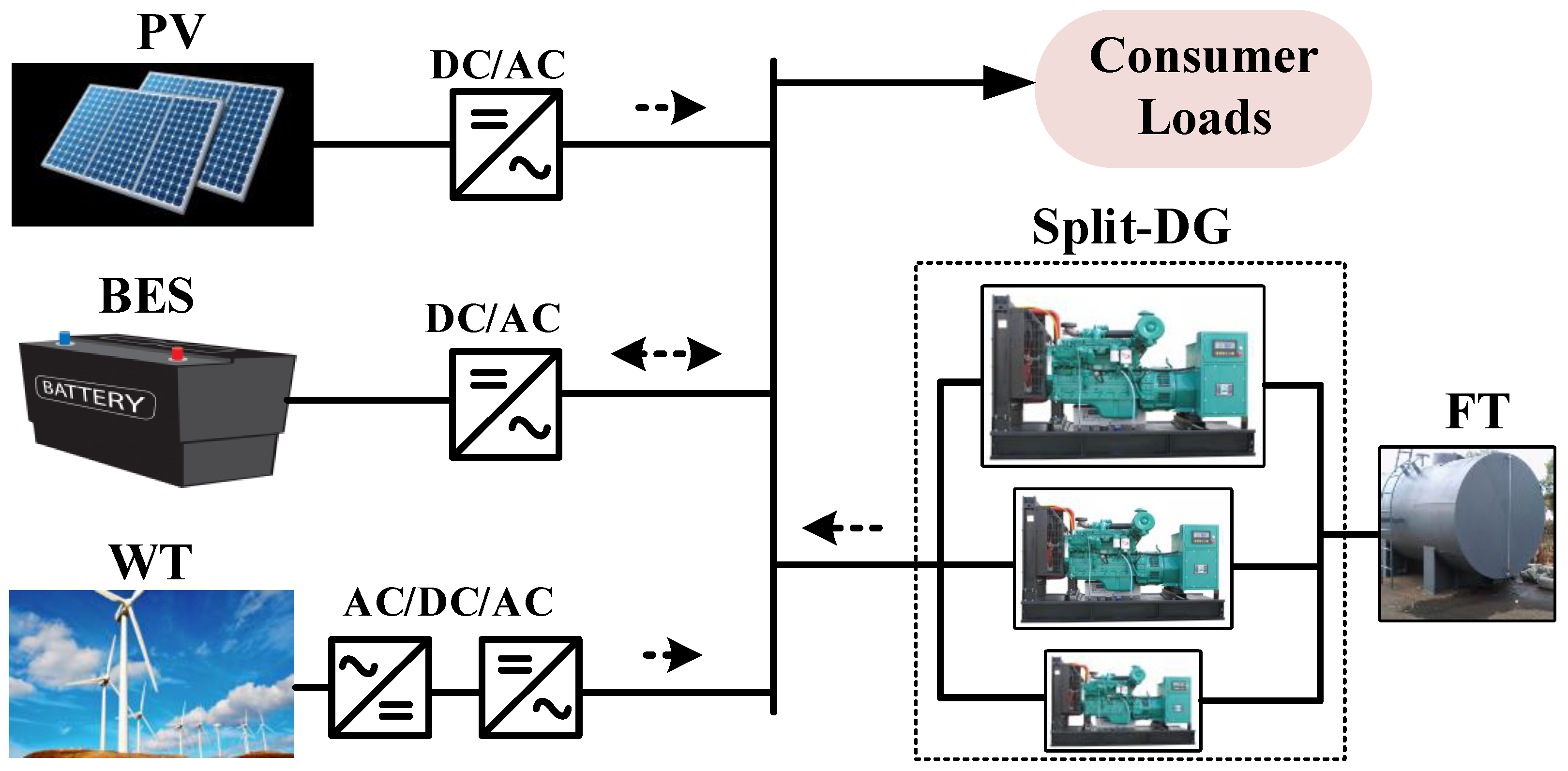
2. System Model

The proposed system in this paper is demonstrated in Figure 1. The system has an AC-coupled architecture to directly supply the load. The PV and BES are connected to the AC-bus through DC/AC converters, and WTs use an AC/AC converter while the Split-DG system and the load are directly connected to the AC bus. The AC-coupled architecture presents some essential advantages for remote areas, such as easy integration into the existing grid, more availability of AC components in local markets, and qualified workers to perform any maintenance or reparation. Additionally, AC-coupled systems present lower copper losses and lower currents than DC-coupled systems [12].

2.1. Model of Components

The models of components are described in this section.

2.1.1. Photovoltaic System

The hourly insolation $I_c$ (kW/m²) and ambient temperature $T_{amb}$ (°C) are evaluated to calculate the output power of the PV system as follows [8]:

$$P_{PV,r}\left(t\right)={\eta }_{pv}{P}_N\left(\frac{I_c\left(t\right)}{I_{stc}}\right)\left(1-\gamma \left(T_{cell}\left(t\right)-T_{stc}\right)\right)$$

(1)

where $I_c$ is composed of the beam, reflective, and diffused isolation on the panels. PVs are assumed to be facing north with a tilt of 30°. Moreover, ${\eta }_{pv}$ and $\gamma$ correspond to the PV’s efficiency and power deratings by temperature, respectively. The cell temperature of solar PV is calculated as follows:

$$T_{cell}\left(t\right)=T_{amb}\left(t\right)+\left(\frac{NOCT-20 °\mathrm{C}}{0.8 \mathrm{kW}/{\mathrm{m}}^2}\right)I_c\left(t\right)$$

(2)

The actual generation of solar PV is calculated based on the number of PV ($N_{pv}$) and the rated power of PV ($P_{PV,r}$) as follows:

$$P_{pv}\left(t\right)=N_{pv}{P}_{PV,r}\left(t\right)$$

(3)

The PV’s degradation is occurred due to the discoloration of the panels. In this study, the PV’s degradation is considered as 0.95% [19].

2.1.2. Wind Turbine

The power generation of a WT is obtained by the wind speed at the hub height that is between the rotational capacities of the WT. The wind speed data used in this study were taken at 10 m height; thus, this speed is corrected to the hub heigh by mean of:

$$v={\left(\frac{H}{H_0}\right)}^{\mathsf{\alpha }}{v}_0$$

(4)

This equation is a relationship of the reference height ($H_0$) and the desired height ($H$) affected by the power of the surface friction coefficient $\alpha$.

The WT requires a minimum wind speed $v_c$ to generate power, which increases by the cube of the wind speed ratio at each time interval until wind speed reaches the rated speed of the turbine $v_r$. From this point, the turbine delivers its rated power when the maximum speed $v_f$ is reached. The generated power by the WT can be calculated as [14]:

$$P_{wt}\left(\mathrm{t}\right)=\{\begin{array}{c}0 ; v<v_c \mathrm{or} v>v_f\hfill \\ {\eta }_{wt}{N}_{wt}{P}_{WT,r}{\left(\frac{v\left(t\right)-v_c}{v_r-v_c}\right)}^3\hfill \\ {\eta }_{wt}{N}_{wt}{P}_{WT,r} ; v_r\le v<v_f\hfill \end{array} ; v_c\le v<v_r$$

(5)

2.1.3. Battery Energy Storage

BES is connected to a bidirectional inverter that allows the charging and discharging of the battery at each time interval. In this study, since the considered system is a residential microgrid and the loads of the system are not sensitive, the microgrid does not require an uninterruptible Power Supply (UPS). It is assumed that the BES works as a UPS in the considered system to cover the intermittent generation of renewable energy sources. Hence, the BES is charged by the extra energy of the RE sources, and then, it is discharged when there is lack of RE generation to supply the load. The state of charge ($SOC$) of the BES is defined by the limits $SO{C}_{min}$ and $SO{C}_{max}$, which corresponds to 20% and 90%, respectively, of the rated capacity of the battery, $E_r^{BB}$. The SOC at each time interval is calculated based on the efficiency of BES and the available input/output energy as follows:

$$SOC\left(t+1\right)=SOC\left(t\right)+\frac{E_{in}^{BB}\left(t\right){\eta }_{BB}-E_{out}^{BB}\left(t\right)/{\eta }_{BB}}{N_{BB}{E}_r^{BB}}$$

(6)

where $N_{BB}$ represents the number of batteries in the BES, ${\eta }_{BB}$ is the total efficiency of the BES, including the efficiency of the bidirectional inverter, and $E_{in}^{BB}$ and $E_{out}^{BB}$ are the input and output energy available for each time interval that are obtained by the input power $(P_{in}^{BB}$) and output power ($P_{out}^{BB}$) of the battery as follows:

$$P_{in}^{BB}\left(t\right)=min\left(P_{max}^{BB},\frac{N_{bb}{E}_{in}^{BB}}{\Delta t}.\frac{SO{C}_{max}-SOC\left(t\right)}{{\eta }_{BB}}\right)$$

(7)

$$P_{out}^{BB}\left(t\right)=min\left(P_{max}^{BB},\frac{N_{bb}{E}_{in}^{BB}}{\Delta t}.\left(SOC\left(t\right)-SO{C}_{max}\right)\left({\eta }_{BB}\right)\right)$$

(8)

The maximum available power of BES is calculated based on the number of batteries and its rated power as follows:

$$P_{max}^{BB}=N_{bb}.P_{BB,r}$$

(9)

The Rainflow Counting Method (RCM) and an experimental model of degradation are used to predict battery lifetime in this study. This method has been successfully applied for battery lifetime estimation and fully explained in [19]. The RCM method counts the number of complete and half cycles by finding all peaks and valleys of the SOC during the whole project period [19]. The total degradation is then calculated to obtain the actual battery’s lifetime. The obtained lifetime from RCM is compared with the calendar lifespan from the manufacturer (20 years) and the lower lifetime is selected.

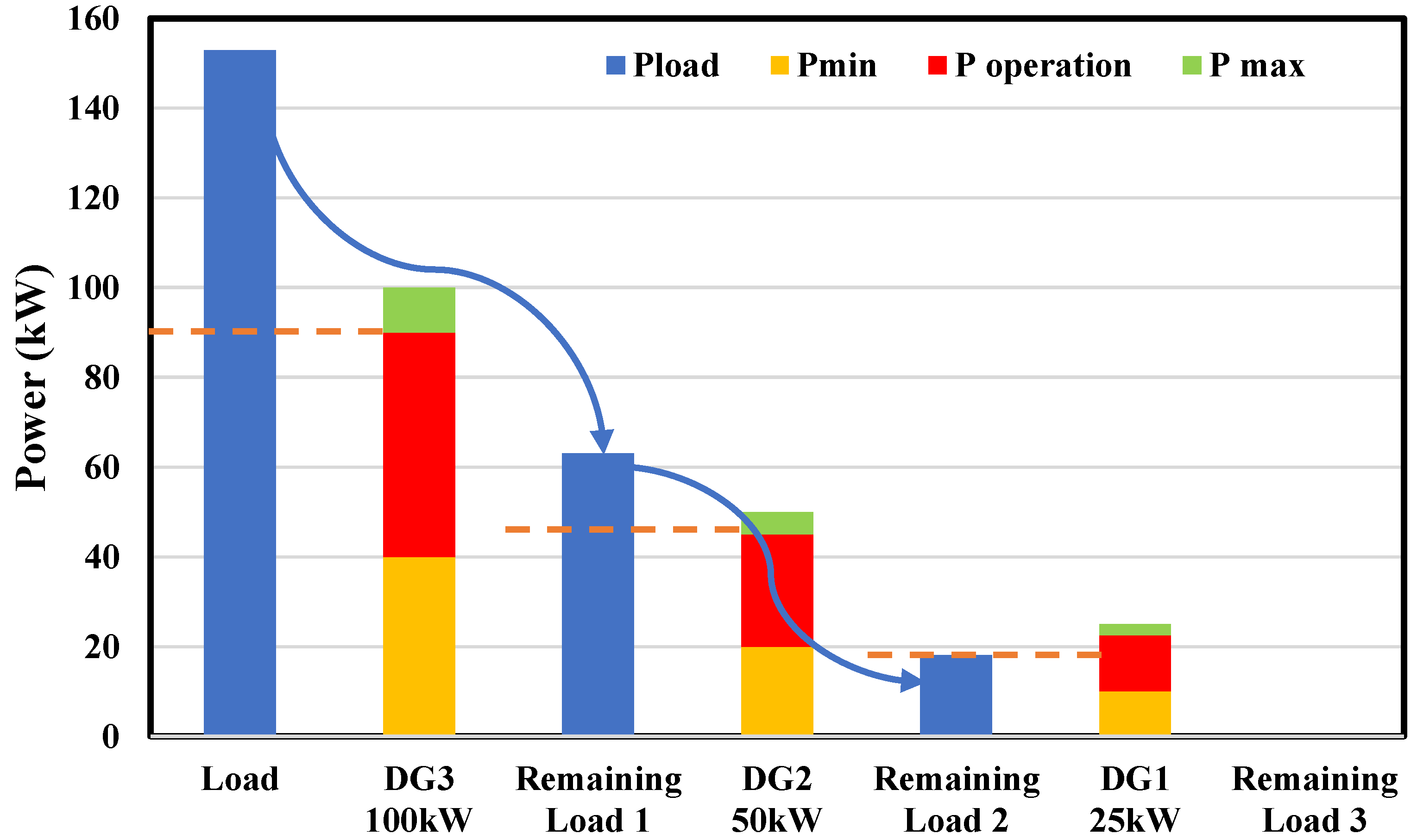
2.1.4. Split-Diesel Generators

Split-DG is a concept introduced as an option to reduce contamination and dumped power of DGs. This study utilizes three different sizes of DGs (25 kW, 50 kW, and 100 kW). These sizes are selected by considering their availability in the local market in case of unexpected replacement or reparation. This consideration aims to reduce the logistic and delivery time to this remote area. The Split-DG control is presented in Figure 2, where each DG is connected to a comparator through switches that are managed by the same comparator. Thus, the comparator senses the required power $\left(P_l\right)$ and the total DG output power $\left(P_{GEN}\right)$ and if $P_l>P_{GEN}$, the comparator changes the configuration K of the switches until $P_l\le P_{GEN}$. The different configurations of the DG’s switches can be observed in Figure 2. Diesel generators control in a Split-DG system, with 1 being ON and 0 being OFF. The control complexity criterion previously mentioned refers to the number of configurations for n number of DGs. The number of switching configurations is obtained as $2^{\mathrm{n}}-1$.

Table 2. Switches configuration for a Slit-DG system.

Combination (k)	${\mathit{S}}_1$	${\mathit{S}}_2$	${\mathit{S}}_3$
1	1	0	0
2	0	1	0
3	0	0	1
4	1	1	0
5	1	0	1
6	0	1	1
7	1	1	1

shows the switches configurations for Split-DG.

For simplicity, it is assumed that all DGs of each type $\left(D{G}^i\right)$ operate in parallel, so the load is supplied equally by the minimum number of on DGs in each time interval ($MinD{G}_{on}^i\left(t\right)$). Additionally, all DGs operate between their operation limits ($D{G}_{max/min}^i)$, as shown in Equation (10):

$$MinD{G}_{on}^i\left(t\right)D{G}_{min}^i{P}_{\mathrm{r}}^{\mathrm{i}}\le P_{\mathrm{DG}}^{\mathrm{i}}\left(\mathrm{t}\right)\le N_{\mathrm{DG}}^{\mathrm{i}}D{G}_{max}^i{P}_{\mathrm{r}}^{\mathrm{i}}$$

(10)

In this operational region, the relationship between L/kWh consumed is almost constant. Thus, all DGs have the same fuel consumption rate. The total diesel generation that corresponds to the summation of all $P_{DG\mathrm{i}}$, with their respective switch configuration for that instant of time, is formulated as follows:

$$P_{DG}^{Total}\left(t\right)=S_1\left(t\right)P_{DG1}\left(t\right)+S_2\left(t\right)P_{DG2}\left(t\right)+S_3\left(t\right)P_{DG3}\left(t\right)$$

(11)

Figure 3 explains the distribution of the $P_l\left(t\right)$ in a three-split-DG system. For this case, a sample load of 153 kW is considered, and it is assumed that there is only one DG of each size. The first, second, and third DG sizes correspond to the rated sizes of 25 kW, 50 kW, and 100 kW, respectively. The biggest available DG supplies the largest portion of the load, considering its maximum output power constraint, 90 kW for DG3. The Remaining Load 1, shown in the figure, is obtained by subtracting the total load and the maximum power of DG3. Then, the DG2 generates its maximum power (45 kW) to supply Load 1. The Remaining Load 2 refers to the last bit of power to be supplied. At this stage, the remaining Load 2 is 18 kW. The operating range of DG1 is between 10 kW and 22.5 kW; thus, DG1 can supply Load 2 without any excess or lack of power. This is the reason that the remaining Load 3 is zero.

2.1.5. Fuel Tanks (FT)

Fuel distribution is a constant constraint in remote areas due to the complex logistic for fuel delivery. Therefore, it is required to predetermine the minimum number of days of fuel $F{T}_{min-days}$ in order to have enough backup in case of any delay in the delivery. The fuel level at each time interval $FV\left(t\right)$ must be inside the maximum and minimum storage volume;

$$F{V}_{min-vol}\le FV\left(t\right)\le N_{FT}F{T}_{vol}$$

(12)

$F{V}_{min-vol}$ must be enough to produce the daily average load for the $F{T}_{min-store}$ as follows:

$$F{T}_{min-vol}=F{T}_{min-days}F{R}_{DG}{P}_l^{Ave}24 \mathrm{h}$$

(13)

2.2. Dumped Power

The dumped power is the extra generated power after load supply and battery charging [5]. The dumped power is produced by the RE resources and online DGs working over their minimum operation point. The dumped power of RE sources can be controlled by the control system of their inverters. The dumped power at each time interval is calculated as shown below [5]:

$$P_{dump}\left(t\right)=P_{DG}^{Total}\left(t\right)+P_{wt}\left(t\right)+P_{pv}\left(t\right)+P_{out}^{BB}\left(t\right)-P_{in}^{BB}\left(t\right)-P_l\left(t\right)$$

(14)

2.3. Spinning Reserve

Spinning reserve (SR) refers to the spare power available to respond to any sudden change in the load or/and the RE. The DGs and BES usually provide SR and inertia in off-grid power systems. DGs working under the rated power have a spare capacity to respond instantaneously to a fluctuation. On the other hand, the RE sources cannot provide SR due to their unstable generation; however, the extra power after feeding the load can be stored in the BES. This energy can be injected rapidly to contribute to the SR, while other DGs are starting to keep up with the demand. This methodology has been used successfully in hybrid power systems.

$$P_{SR}\left(t\right)=MinD{G}_{on}^1\left(t\right)P_{rDG1}+MinD{G}_{on}^2\left(t\right)P_{rDG2}+MinD{G}_{on}^3\left(t\right)\left(t\right)P_{rDG3}+P_{out}^{BB}\left(t\right)-P_{LOAD}\left(t\right)$$

(15)

2.4. CO₂ Emission

Since carbon dioxide (CO₂) makes up the majority of greenhouse gas emissions (GHG) from the electricity sector [20], the term CO₂ emission has been used in this study instead of GHG. The total CO₂ emission ($E_{C{O}_2}^{Total}$) is calculated from the total diesel consumed by the DGs during the whole year and an emission rate ($E{R}_{C{O}_2}$) of 2.7 kg/L [21]:

$$E_{C{O}_2}^{Total}=E{R}_{C{O}_2}.{\displaystyle \sum }_{t=1}^{8760}D{G}_{Fuel}\left(t\right)$$

(16)

As it is assumed that all three DGs have the same consumption ratio per generated kW ($F{R}_{DG})$, and the consumed fuel is obtained by the multiplication of the total DGs’ power in each hour, as shown in Equation (11), and $F{R}_{DG}$ as shown below:

$$D{G}_{Fuel}\left(t\right)=F{R}_{DG}.P_{DG}^{Total}\left(t\right)$$

(17)

3. Optimization Model

This study pretends to obtain the most economical hybrid power system using NPV as the objective function. The NPV takes all the expenditures and revenues during the project lifetime and converts them to a present value. The factors considered for the analysis of NPV are the present values of capital cost, replacement cost, regular maintenance cost, and salvation cost of each component, as well as the present values of fuel cost and large-scale generation certificates (LGC) incentive. The NPV of hybrid microgrids is calculated as follows:

$$NPV={\displaystyle \sum }_j{N}_j\left(P{V}_{cap}^j+P{V}_{O\&M}^j+P{V}_{rep}^j-P{V}_{SV}^j\right)+P{V}_{fuel}-P{V}_{LGC}$$

(18)

where j represents the components of the hybrid power system.

The present capital cost is the initial investment cost for each component ($C_{cap}^j$) that should be paid at the beginning of the project:

$$P{V}_{cap}^j=C_{cap}^j$$

(19)

The regular maintenance cost is paid annually during the project lifetime. Hence, its presence can be calculated as follows:

$$P{V}_{O\&M}^j=C_{O\&M}^j\frac{{\left(1+x\right)}^{L{T}_{proj}}+1}{x{\left(1+x\right)}^{L{T}_{proj}}}$$

(20)

The present replacement cost of the components is paid once the component should be replaced due to its lifetime. This cost is formulated as follows:

$$P{V}_{rep}^j=C_{rep}^j\frac{1}{{\left(1+x\right)}^{L{T}_{com}^j}}$$

(21)

The salvation value is the remaining component’s value at the end of the project and is calculated as follows:

$$P{V}_{SV}^j=P{V}_{cap}^j\frac{L{T}_{rem}^j}{L{T}_{com}^j}\frac{1}{{\left(1+x\right)}^{L{T}_{proj}}}$$

(22)

$$L{T}_{rem}^j=L{T}_{proj}-R_{com}^{j}L{T}_{com}^j$$

(23)

where $L{T}_{rem}^j$, $L{T}_{com}^j$, $L{T}_{proj}$, and $R_{com}^j$ are the remaining lifetime of the component at the end of project, component’s lifetime, project’s lifetime, and the number of replacements, respectively.

The present value of the fuel cost is calculated as follows:

$$P{V}_{fuel}=\left(C_{fuel}{\displaystyle \sum }_{t=1}^{8760}D{G}_{Fuel}\left(t\right)\right)\frac{{\left(1+u\right)}^{L{T}_{proj}}+1}{u{\left(1+u\right)}^{L{T}_{proj}}}$$

(24)

where $u$ is the real interest rate for fuel cost which is calculated based on the interest rate and escalation rate and $C_{fuel}$ is the fuel cost for each litre of consumption by the DGs.

The present value of LGC is calculated as follows:

$$P{V}_{LGC}=\left(C_{LGC}{\displaystyle \sum }_{t=1}^{8760}\left(P_{wt}\left(t\right)+P_{pv}\left(t\right)\right)\right)\frac{{\left(1+u\right)}^{L{T}_{proj}}+1}{u{\left(1+u\right)}^{L{T}_{proj}}}$$

(25)

where $C_{LGC}$ is the economic incentive provided by the Australian government to accredited large scale RE generation plants which is considered as 4 ¢/kWh [22].

Evaluation of the hybrid microgrids requires a series of constraints to ensure the desired performance. The constraints defined for this study are:

• All components must operate inside their upper and lower boundaries. These boundaries have been specified in previous sections.
• Load requirement must always be supplied at each time interval.

$$P_l\left(t\right)\le P_{DG}^{Total}\left(t\right)+P_{wt}\left(t\right)+P_{pv}\left(t\right)+P_{out}^{BB}\left(t\right)$$

(26)

• SOC at the end of the analyzed year cannot be less than the initial SOC. The initial SOC at the beginning of the project is predefined as 70%.

$$SOC\left(8760\right)\ge SOC\left(t=0\right)$$

(27)

• There must always be a minimum spinning reserve of 100 kW after the load demand is supplied. This is due to the N-1 reliability index, which should consider the power rate of the largest generation unit of the system. Hence, the SR can be calculated as follows:

$$P_{SR}\left(t\right)\ge P_{DG3}+P_{DG}^{Total}\left(t\right)+P_{wt}\left(t\right)+P_{pv}\left(t\right)+P_{out}^{BB}\left(t\right)-P_l\left(t\right)$$

(28)

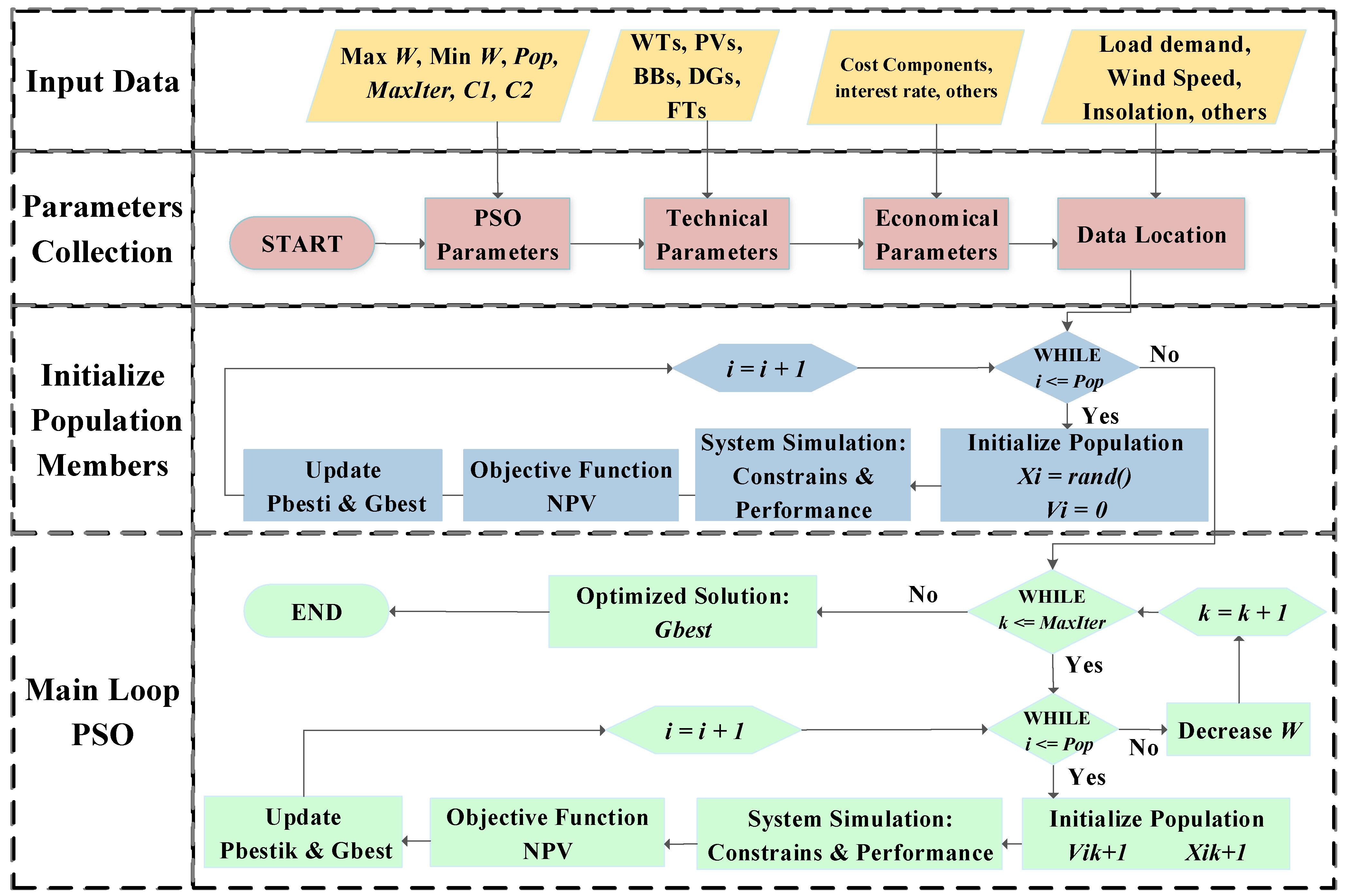
4. Optimization Algorithm

In this study, a variable weighting particle swarm optimization algorithm is proposed to solve the optimization problem. The PSO algorithm has shown a remarkable performance in sizing of microgrids due to its simple implementation, fast convergence, and low dependency on the initial values [23]. The PSO is counted as a bee swarm behavior looking for food. In this study, each particle of PSO represents the number of units of a possible power hybrid configuration, and the food is the NPV. The i-numbers of particles are initially generated randomly inside a search space, recording their position ${\mathrm{x}}_{\mathrm{i}}$ and velocity ${\mathrm{v}}_{\mathrm{i}}$, which is zero for the first iteration. Particles’ positions and velocity vectors are defined as ${\mathrm{x}}_{\mathrm{i}}\in ℝ\ge 0$ and ${\mathrm{v}}_{\mathrm{i}}\in ℝ\ge 0$, respectively, where position and velocity of N-types of components in the HPS are stored as follow: ${\mathrm{x}}_{\mathrm{i}}=\left[{\mathrm{X}}_{\mathrm{i},1},{\mathrm{X}}_{\mathrm{i},2},{\mathrm{X}}_{\mathrm{i},3},\dots ,{\mathrm{X}}_{\mathrm{i},\mathrm{N}}\right]$ and ${\mathrm{v}}_{\mathrm{i}}=\left[{\mathrm{V}}_{\mathrm{i},1},{\mathrm{V}}_{\mathrm{i},2},{\mathrm{V}}_{\mathrm{i},3},\dots ,{\mathrm{V}}_{\mathrm{i},\mathrm{N}}\right]$. For each iteration $\left(\mathrm{k}\right)$, velocity and position are updated, recording the best individual position ${\mathrm{P}}_{\mathrm{best}}$ and the global best solution ${\mathrm{G}}_{\mathrm{best}}$. Once the total number of iterations is reached, the last value obtained in ${\mathrm{G}}_{\mathrm{best}}$ is the optimal solution of the system with the lowest NPV. This process can be observed in detail in Figure 4. The velocity and position are updated in each iteration as follows:

$$v_i^{k+1}=w{v}_i^k+C_1{r}_1\left(Pbes{t}_i^k-x_i^k\right)+C_2{r}_2\left(Gbes{t}_i^k-x_i^k\right)$$

(29)

$$x_i^{k+1}=x_i^k+v_i^k$$

(30)

where $C_1$ and $C_2$ are positive coefficients that accelerate personal and global exploration learning. These positive coefficients are selected so that $C_1+C_1\le 4$ [23]. The social and personal components of the system are balanced when these two parameters are equal [23]. As an error, sometimes when the selection of $C_1$ and $C_2$ are not correct, the final solution could get stuck in personal solutions when $C_1>C_2$. On the other hand, when $C_1<C_2$, the convergency could fail [24]. Additionally, $r_1$ and $r_2$ are random numbers between 0 and 1 that are used to maintain the stochastic distribution of the swarm.

In conventional PSO, the $w$, which is the inertia weight index in which the particle is moving in the search space, is constant. However, the major advantage of the VW-PSO is the capability to adopt $w$. This variable is used to control the strong variations of the $x_i$ that could force the particle to move out of the search space. As a strategy to improve the accuracy and speed of convergency, it is proposed to decrease $w$ in each iteration to limit the particles’ movement at the end of the iterative process. Hence, in each iteration $k$, the weight index is updated as follows:

$$w^k=w_{max}-k\left(\frac{w_{max}-w_{min}}{k^{max}}\right)$$

(31)

It is important to highlight that the optimization problem in this study contains constraints. Therefore, the particles must accomplish all the system’s constraints to be evaluated by the objective function. Otherwise, the unsuccessful particles are penalized with a very large NPV avoiding interferences with the selection of the $G_{best}$ and $P_{best}$. The parameters and values used for PSO were taken from the same case study in [12] and adjusted for this research (see

Table 3. Considered PSO parameters for optimal sizing problem.

Parameter	Symbol	Value
Population	$nPOP$	500
Iterations	$k^{max}$	100
Minimum search space limit	$x_{min}$	0
Maximum search space limit	$x_{max}$	20,000
Maximum variable inertia	$w_{max}$	0.7
Minimum variable inertia	$w_{min}$	0.1
Fixed inertia	$w_{fixed}$	0.5
Personal and Global coefficient	$C_1 and C_2$	2
Number of variables or components	$N$	4–7

). The logical functioning of PSO with the variable weighting factor is shown in Figure 4.

5. System Configurations and Input Data

Three system configurations are examined in this study for optimal sizing. While the first configuration is based only on generation from diesel (Split-DG), the second configuration uses only RE with BES (WT-PV-BES). The third configuration combines both diesel generation and RE. An additional scenario with single-sized DG is used only for comparison with the proposed Split-DG performance.

5.1. Configuration 1

The first configuration is based only on generation from diesel (Split-DG). In this scenario, a three-Split-DG with a rated capacity of 25 kW, 50 kW, and 100 kW are used to supply the whole load and the spinning reserve. The functionality of the Split-DG has been already described. Since this system has no RE sources, it would have the most emission among the proposed system configurations.

5.2. Configuration 2

The second configuration uses only RE with BES. This configuration uses WTs and PVs for power generation and load supply. The BES is added to store the excess energy of REs to use in those moments that the generation is lower than the demand. The BES must guarantee the spinning reserve all the time. This available spare power after feeding the load depends directly on $P_{out}^{BB}$. This system has no emission, and all the load is supplied by RE sources.

5.3. Configuration 3

The third configuration combines both Split-DG generation and RE. This configuration prioritizes the utilization of energy from RE and BES rather than the Split-DG. This approach aims to reduce the consumption of diesel. Split-DG provides the remaining load after using first the available outputs of RE and BES. This remaining portion of the load is re-evaluated to find the most suitable Split-DG configuration. Spinning reserve is provided by the spare power of the minimum number of DGs ON and the available output power of the BES after the load is supplied.

5.4. System Input Data

Actual annual data, which are hourly arranged, are used for optimization. It is essential to highlight that this study uses one-year data, assuming this scenario is repeated until the end of the project’s lifetime. However, this research has considered the annual load growth, as well as the degradations of PV and BES during the lifetime of the project.

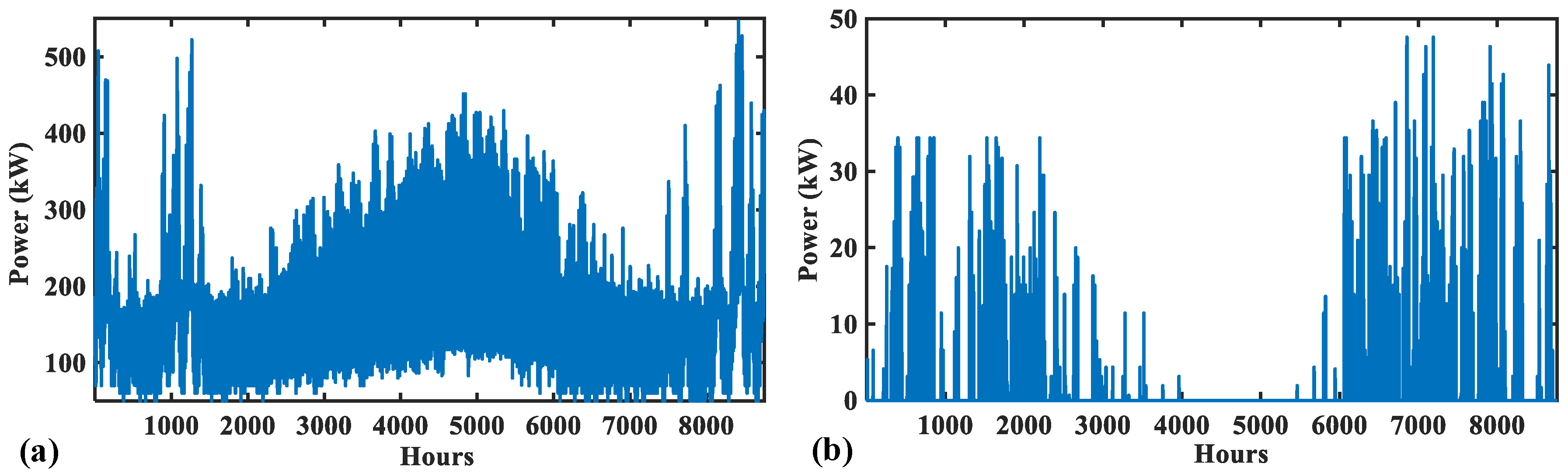
5.4.1. Load Characteristic

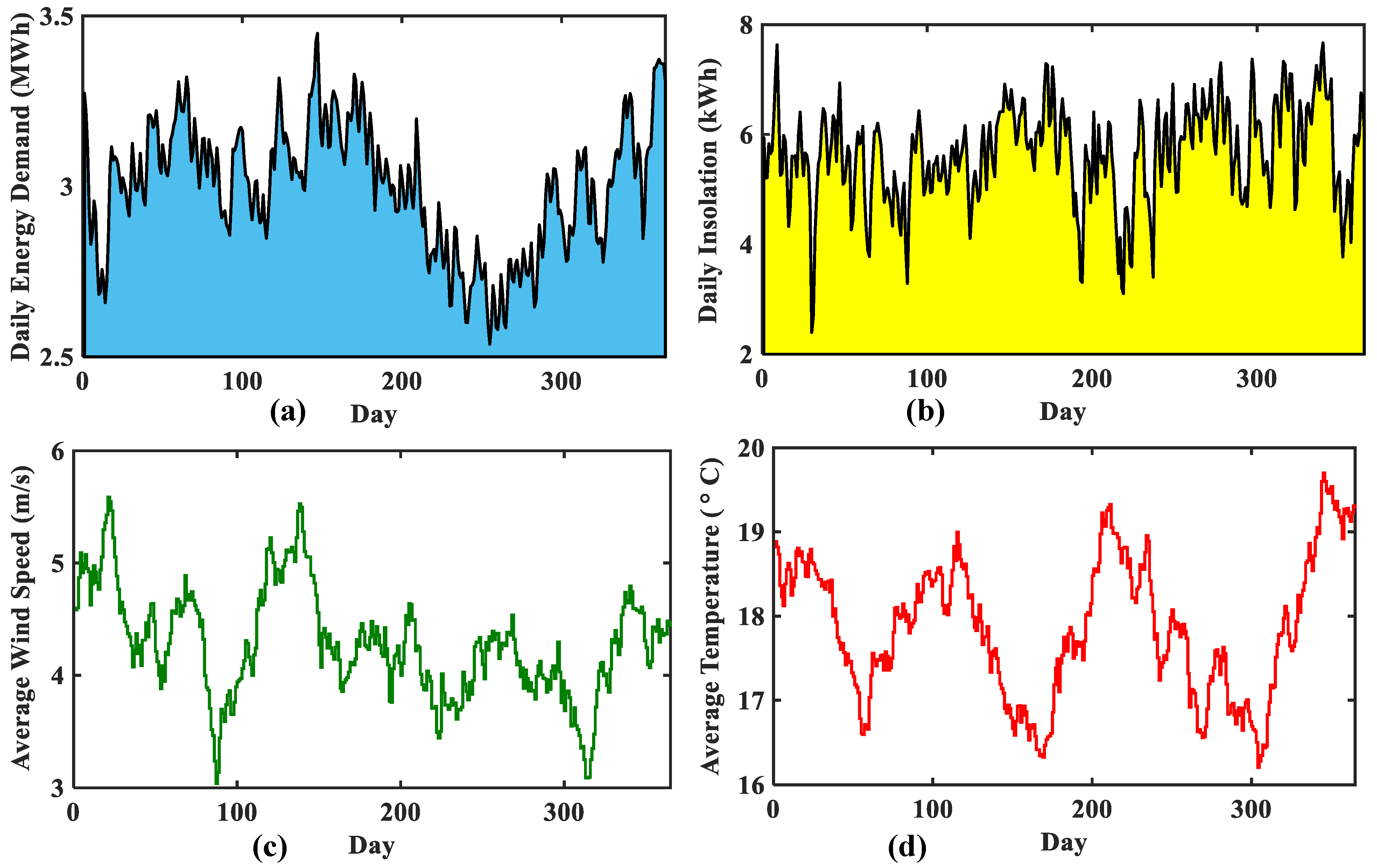
Yalata and Nundroo are small aboriginal communities with 65 and 48 users located in a remote area in the north-west of South Australia. Currently, each community is powered by an independent local off-grid diesel power station. These two communities are close enough to consider a single solution for both places. It is stated from a technical report that the expansion of the national grid to these locations would cost around AUD 15 million. This expansion was discarded due to the lower recovery cost per capital of the project. Even though this area has good potential for WTs and PVs, these two places are currently dependent on diesel power plants.

Historical data has shown that this region’s population’s growth ranges from 0% to 5% [25]. Due to the small size of these communities with residential load-profile, the load’s growing ratio is assumed as 1% per year. Figure 5a shows the daily energy demand through the year by considering the load growth after 20 years. The total annual energy consumption is 1336 MWh, while maximum, minimum, and average power consumptions are 546.64 kW, 2.44 kW, and 152.52 kW, respectively.

5.4.2. Weather

Due to the closeness of these two communities, the weather variations are not significant to consider them independently; however, there is no exact meteorological information of these lands. Thus, this information has been taken from a 10-year meteorological report of these lands Port Augusta [26]. Port Augusta is located around 550 km away from Nundaroo and Yalata, but by observing the meteorological record of both sites, both places have similar weather behavior. Therefore, corrections to the insolation have been applied by using the coordinates of the studied location. The daily solar insolation, daily average wind speed, and daily average temperature are demonstrated in Figure 5b–d. From weather data in Figure 5, it is clear that this remote area has potential for the use of RE.

Table 4. Annual average, minimum, and maximum of weather data.

	Annual Average	Maximum	Minimum
Wind Speed (m/s)	4.3	11.5	0
Insolation (Wh/m2)	431.7	1015	0
Ambient Temp (°C)	17.9	41.9	2.2

summarizes the maximums, minimum, and annual average of wind speed at 10 m heigh, solar irradiation, and ambient temperature at this area.

The average diesel price for remote areas, including the delivery and the Fuel Tax Credit, is around AUD 1.30/L [1]. Additionally, the prices of fuels have been increasing throughout time, so an annual increment rate of 2% is assumed to emulate this tendency [16].

5.4.3. Components’ Data

Table 5. Components’ parameters in this study.

Specification	Symbol	Quantity	Specification	Symbol	Quantity
Diesel Generator 1			Wind Turbine
Nominal power	$P_{\mathrm{r}DG1}$	25 kW	Nominal power	$P_{\mathrm{r}WT}$	10 kW
Min. Operation	$\mathrm{DG}{1}_{\min }$	40%	Wind speed cut-in	$v_c$	3 m/s
Max Operation	$\mathrm{DG}{1}_{\max }$	90%	Wind speed nominal	$v_r$	12 m/s
Fuel consumption	$F{R}_{DG}$	0.3 L/kWh	Wind speed cut-out	$v_f$	25 m/s
Lifetime	$L{T}_{DG1}$	10 years	Hub height	$H$	25 m
Capital cost		AUD 5250	Friction coefficient	$\mathsf{\alpha }$	0.4
Replacement cost		AUD 5250	Efficiency	${\eta }_{wt}$	88%
O&M cost		AUD 525	Lifetime	$L{T}_{WT}$	10 years
Diesel Generator 2			Capital cost		AUD 30,000
Nominal power	$P_{\mathrm{r}DG2}$	50 kW	Replacement cost		AUD 3000
Min. Operation	$\mathrm{DG}{2}_{\min }$	40%	O&M cost		AUD 100
Max Operation	$\mathrm{DG}{2}_{\max }$	90%	Photovoltaic Array
Fuel consumption	$F{R}_{DG}$	0.30 L/kWh	Nominal power	$P_{\mathrm{r}PV}$	1 kW
Lifetime	$L{T}_{DG2}$	10 years	Cell temperature STC	$T_{stc}$	25 °C
Capital cost		AUD 10,500	Cell temperature NOCT	$NOCT$	45 °C
Replacement cost		AUD 10,500	Temperature derating		0.4%/°C
O&M cost		AUD 1050	Efficiency	${\eta }_{PV}$	86%
Diesel Generator 3			Degradation	g	0.95%/year
Nominal power	$P_{\mathrm{r}DG3}$	100 kW	Tilt angle		30°
Min. Operation	$\mathrm{DG}{3}_{\min }$	40%	Azimuth		0°
Max Operation	$\mathrm{DG}{3}_{\max }$	90%	Lifetime	$L{T}_{PV}$	10 years
Fuel consumption	$F{R}_{DG}$	0.30 L/kWh	Capital cost		AUD 1500
Lifetime	$L{T}_{DG3}$	10 years	Replacement cost		AUD 300
Capital cost		AUD 21,000	O&M cost		AUD 25
Replacement cost		AUD 21,000	Battery Bank
O&M cost		AUD 2100	Nominal power	$P_{\mathrm{r}BB}$	0.4 kW
Fuel Tank			Nominal energy	$E_{\mathrm{r}BB}$	1 kWh
Nominal capacity	$F{T}_{vol}$	10 kL	Min. SOC	${\mathrm{SOC}}_{\min }$	20%
Min. days of storage	$F{T}_{min-day}$	7 days	Max. SOC	${\mathrm{SOC}}_{\max }$	90%
Frequency refill		30 days	Initial SOC	${\mathrm{SOC}}_{\mathrm{ini}}$	70%
Lifetime	$L{T}_{FT}$	20 year	Efficiency	${\eta }_{BB}$	91%
Capital cost		AUD 40,000	Lifetime	$L{T}_{BB}$	20 year
Replacement cost		AUD 30,000	Capital cost		AUD 600
O&M cost		AUD 1000	Replacement cost		AUD 400
			O&M cost		AUD 10

contains the technical and economic summaries of the components considered in this study. Efficiencies of inverters, converters, and wiring losses are included in the total efficiency of each component that connects to the AC-bus.

6. Results and Discussions

This section presents the optimization results of the system configurations. The NPV fraction as well as the annual and daily operation of the system configurations are indicated. The proposed systems are compared with the conventional single-DG system and the optimized systems by the conventional PSO algorithm. Note that the currency of all costs shown in this study is Australian Dollars.

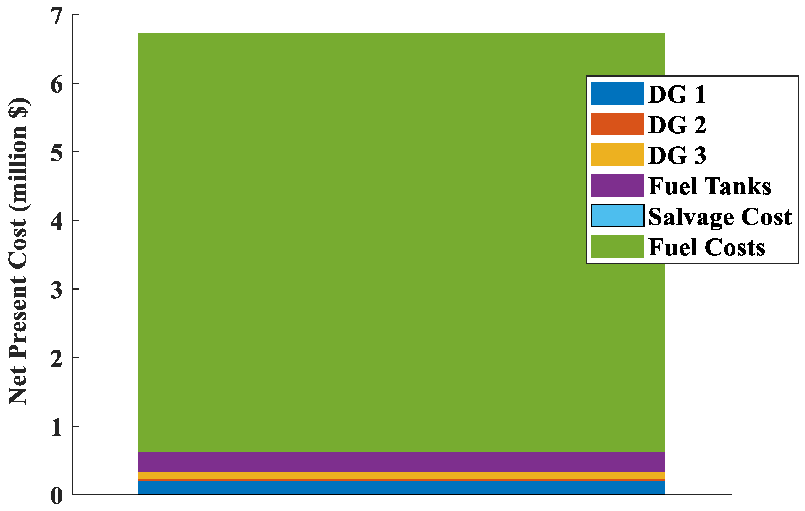
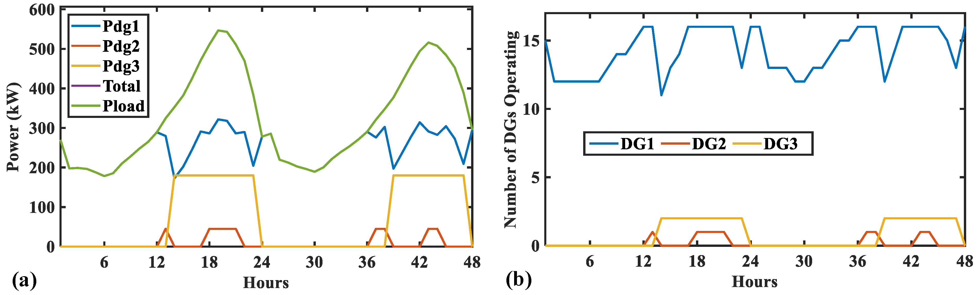
6.1. Configuration 1

Table 6. Optimal results for Configuration 1.

Configuration [DG1, DG2, DG3, FT]	NPV (AUD Million)	Diesel Generation (MWh)	Fuel Consumption (kL/Year)	Dumped Energy (MWh)	CO2 Emissions (Tonne/Year)
[16, 1, 2, 6]	6.733	1350.74	405.22	14.65	1094

lists the optimal results obtained from the VW-PSO for Configuration 1. The system’s NPV for 20-year operation is AUD 6.733 million. This solution has a rated capacity of 650 kW with 16, 1, and 2 numbers of DG1, DG2, and DG3, respectively. Six fuel tanks are required to store up to 60 kL in total. The system consumes 405.22 kL fuel per year, which results in 1094 tonne CO₂ emission per year. The annual dumped energy is 14.65 MWh for Configuration 1.

Figure 6 indicates the NPV fraction of the optimized solution for Configuration 1. All DGs are replaced once in the middle of the project, and the second replacement is at the same time as the project lifetime. A similar scenario happens for FTs which have a 20-year lifetime. Therefore, no salvation value is included in the NPV of DGs and FT. As this configuration is based only on diesel, around 90% of NPV is composed of the fuel consumption during the whole project. Note that diesel prices increase gradually at a rate of 2%, which means that at the end of the project, cost increases around 63 ȼ/L.

Figure 7 shows the annual operation of Configuration 1 for diesel generation and dumped power. As shown, the Split-DG generation follows the load consumption. The power dumped is occurred due to generation constraint of the DGs. The highest dumped power is 50 kW through the year.

It is important to check the proper operation of the system based on a daily operation. For this purpose, a time interval has been selected that corresponds to the 48 h where the maximum peak demand occurs. Figure 8a demonstrates that the generation in Configuration 1 perfectly follows the load even during the peak time. As explained in previous sections, all DGs of the same size work in parallel, delivering the same power in-between their optimal operational limits.

Figure 8b shows the number of diesel generators running at each time interval. During this period of high demand, there are always at least 11 DG1s running, feeding the load, and guarantying the spinning reserve. As the load increases, the number of DG1 increases to the maximum, which is 16, then DG2 and DG3 are brought online as required. After 13 h, the load plus the spinning reserve is greater than the maximum power delivered by the 16 DG1; thus, it is required to start the DG2 until the combined generation is not enough for the demand. In this case, two of DG3s are brought online as the load reaches its peak. This scenario clearly shows how multiple sizes of DGs work together to feed the load minimizing the use of diesel and dumped power.

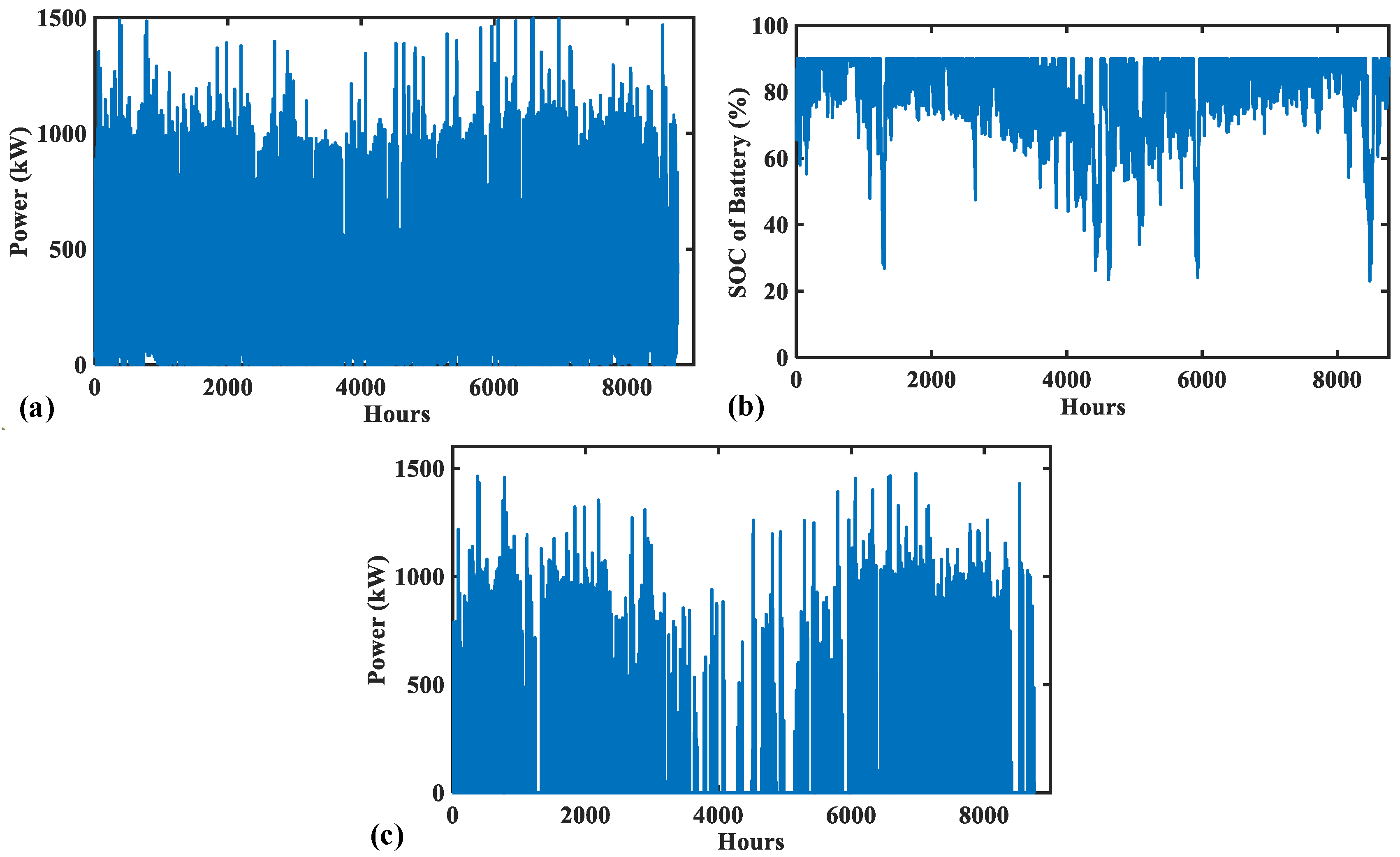
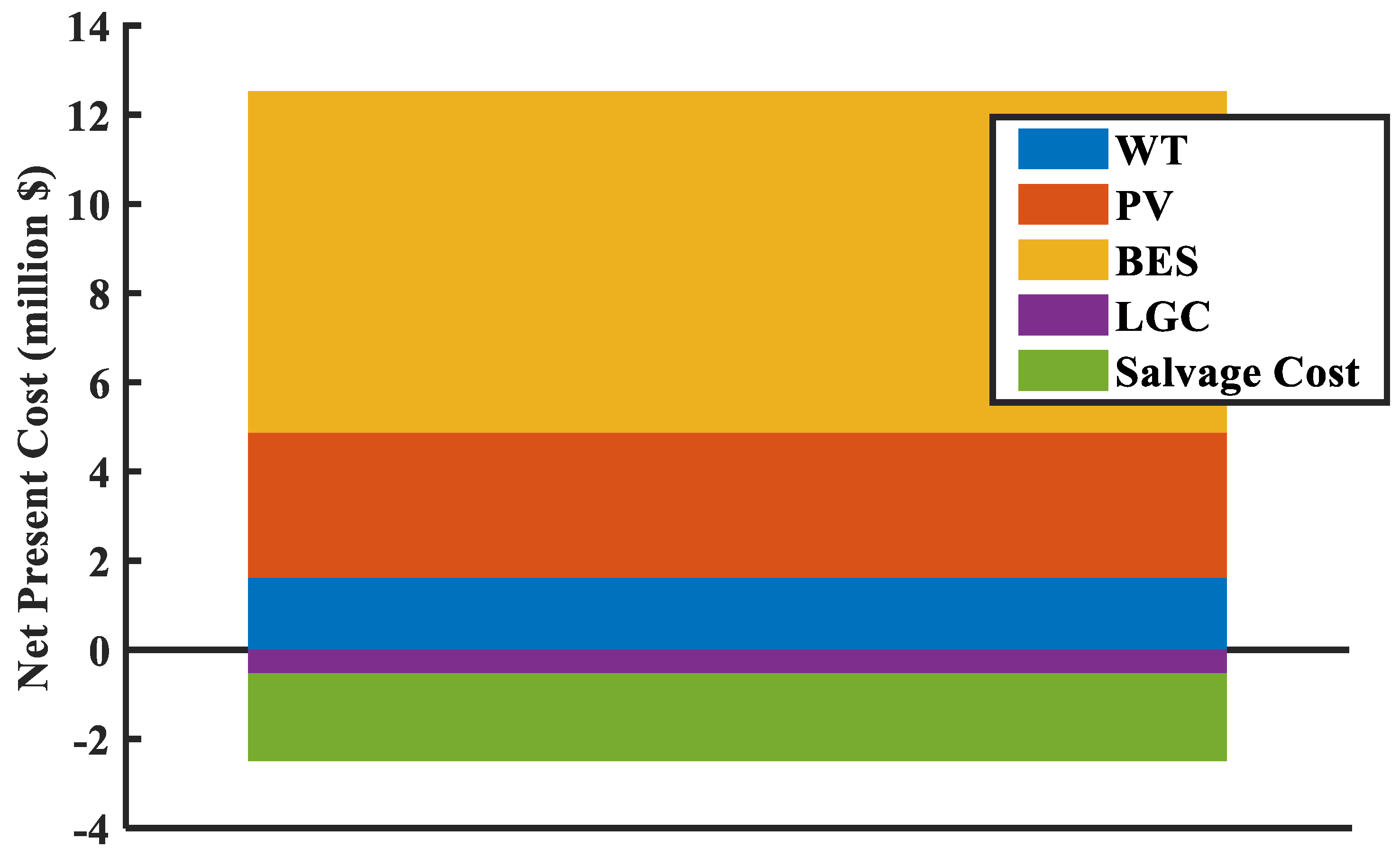
6.2. Configuration 2

Table 7. Optimal results for Configuration 2 (PV-WT-BES).

Configuration [WT, PV, BES]	NPV (AUD Million)	Energy Generated (MWh)	PV Energy (MWh)	WT Energy (MWh)	BES Charging (MWh)	BES Discharging (MWh)	Dumped Energy (MWh)
[50, 1728, 10,956]	10.03	2833.80	2243.61	590.18	766.75	633.01	1363.96

summarizes the performance of the optimized solution for Configuration 2 (PV-WT-BES). It requires high capacity of each component to guaranty the load supply at any time. The BES plays an important role in this configuration because it manages the spinning reserve required for the system. In this case, 48.08% of the total generated RE is wasted. About 27.1% of the total RE was charged in the storage system, which supplied 57.81% of the load. This configuration relies notably on the PV array providing 79.16% of the total energy. This justifies the large number of PVs and BESs. The system, basically, stores as much energy as possible during the day to be used during the nights. From an economic point of view of the optimized solution for Configuration 2, the NPV of the 20-year project in this scenario is AUD 10.03 million. This NPV is reduced by AUD 2.25 million compared to Configuration 1. This NPV reduction is due to the Large-Scale Certificate incentive and the Salvage Cost.

Figure 9 shows that the most significant portions of the NPV come from the BESs and PVs with AUD 6.70 million and AUD 3.25 million, respectively. However, the only component contributing to the salvation value is the BES because battery is the only component that its lifetime does not match with the project lifetime. The remaining BES’s lifetime at the end of the project is nine years.

Figure 10a shows the total generation produced by the WT and PV. It is observable that the system generates high power, reaching almost 1.5 MW in some times; however, it is clear that because of the variability of RE, the generation drops to zero in some times. The large storage system is obtained due to the lack of generation during high power demand. Figure 10b presents the SOC of the BES, which does not exceed 90% and 20% as specified in the constraints section. The annual average of the SOC is obtained as 79.38%. It is observable that the SOC decreases notably during the peaks of demand in summer and during the average increment in winter. Figure 10c shows that there is high dumped power most of the year except during winter when the PV generation is low. Therefore, this RE system needs to be oversized to supply the studied load.

Configuration 2 is entirely powered by PVs and WTs with a storage system. The PV system (2243.61 MWh) produced the most considerable energy, while WTs just contributed 590.18 MWh during the whole year. This scenario can be seen in Figure 11a during a 48-h operation of the highest peak of load. Although the load is successfully supplied, a large portion of energy cannot be collected by the BES, as shown in Figure 11b. This graph is straightforward to show the charging process during the day and the discharging at night. The large size of BES ensures enough energy to manage any load variation.

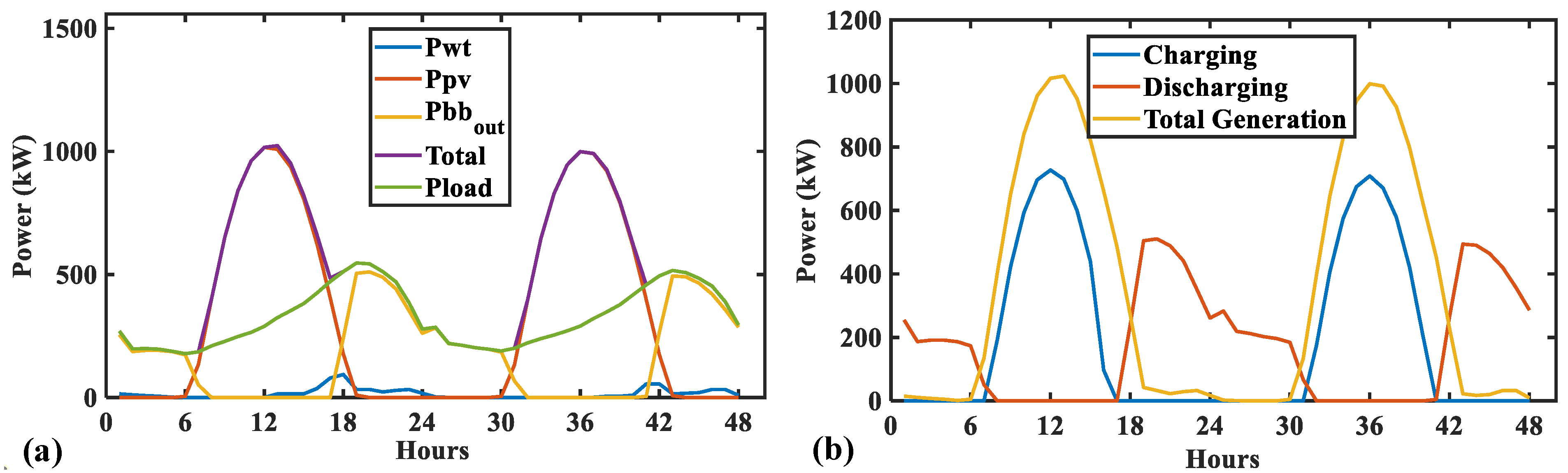
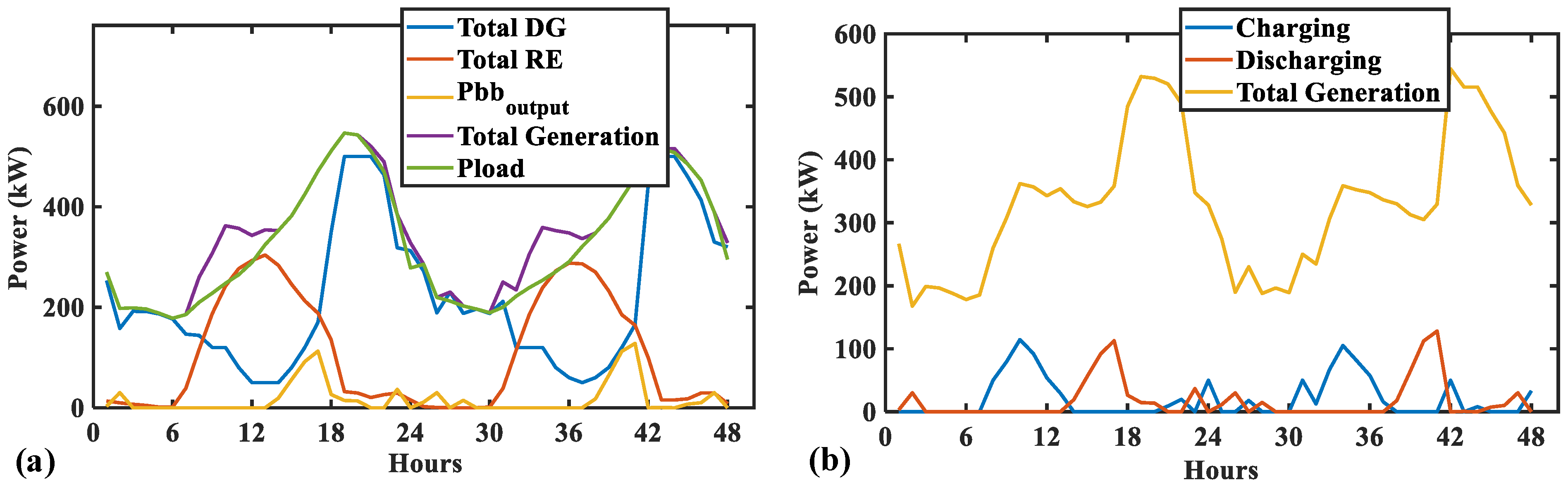
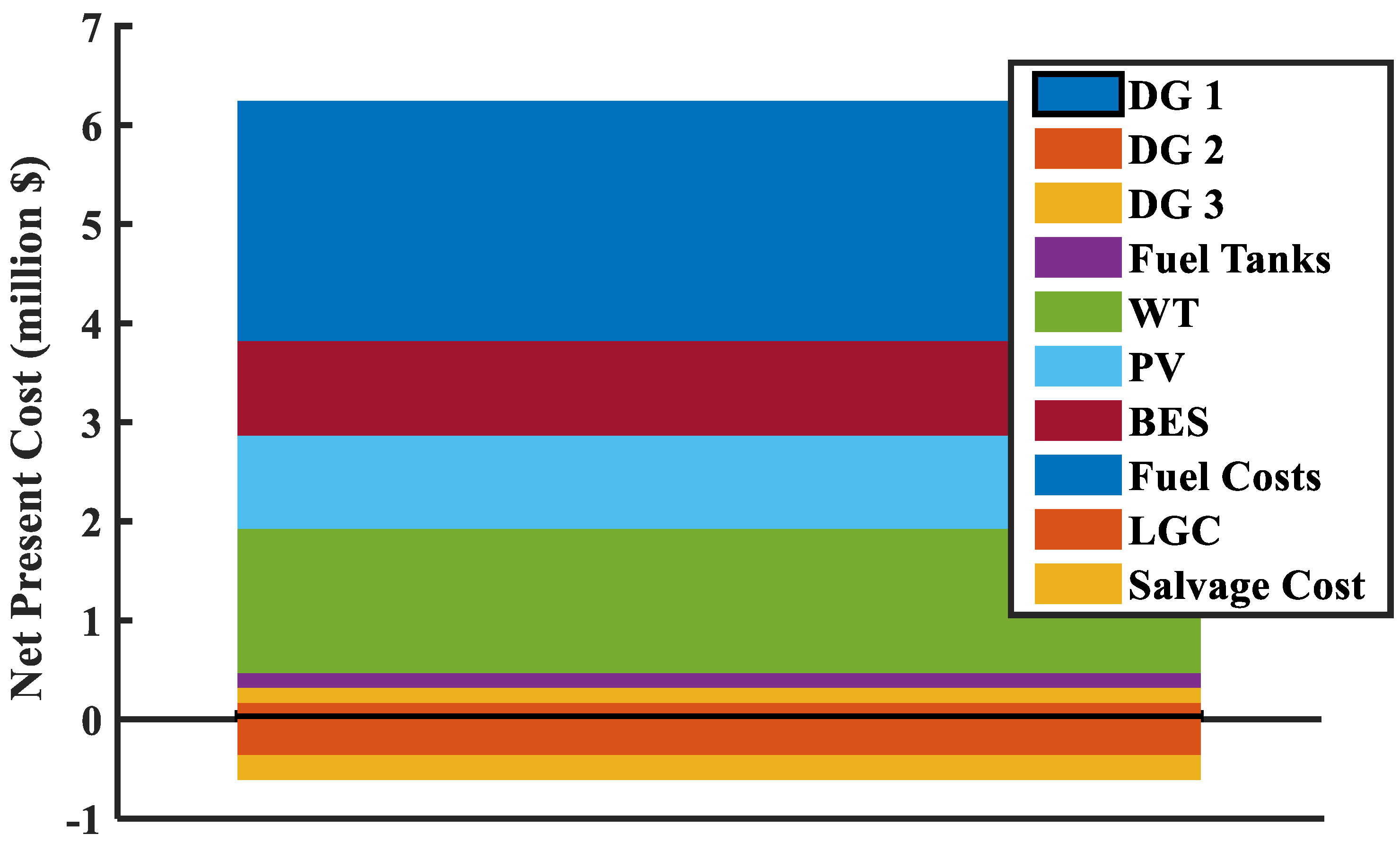
6.3. Configuration 3

Configuration 3 combines all the components from Configuration 1 and 2.

Table 8. Optimized solution for Configuration 3 (Split-DG-PV-WT-BES).

Configuration [DG1, DG2, DG3, FT, WT, PV, BES]	NPV (AUD Million)	Diesel Generation (MWh)	RE Energy (MWh)	RE Index (%)	Dump Energy (MWh)	Fuel (L/Year)	CO2 (Tonne/Year)
[5, 4, 3, 3, 45, 498, 1372]	5.634	535.54	1177.8	68.74	320.86	160.66	433.78

lists the optimal results for Configuration 3. The RE index shows the portion of the load, which is supplied by the RE generation rather than diesel generation. While the combined generation of the WTs and PVs accounted for 1177.8 MWh/year, the Split-DG system generated 535.54 MWh/year. The RE system supplies 68.74% of the total load. However, this solution presents a significant dumped energy of 320.86 MW/year, which is 18.72% of the total generation. Additionally, this configuration requires three FTs to feed five DG1, four DG2 and three DG3. The total fuel consumption throughout the year is 160.66 kL, producing 433.78 tonnes of CO₂.

Figure 12 illustrates the NPV fraction of the optimized solution for Configuration 3. The NPV of fuel is the most significant contributor, with AUD 2.42 million, followed by the NPV of WTs, BESs, and PVs with AUD 1.46 million, AUD 0.96 million, and AUD 0.94 million, respectively. In this scenario, selling the 1372 batteries with a remaining lifetime of 8 years reduces the NPV by AUD 247,000 at the end of the project lifetime. In addition, the LGC credit for producing 1177.8 MWh ascends to AUD 360,000.

Figure 13a shows the total RE generation, which varies notably from zero to a maximum power generated of 701 kW provided mainly by the PV system. On the other hand, the Split-DG system supports the RE generation, as shown in Figure 13b. Comparing Figure 13b,c shows that the BES system is more active for injecting power rather than the Split-DG. However, it is obvious that the Split-DG system contributes to supply the deficit during the high demand periods and maintains the spinning reserve. The BES stored about 19.13% of the total generated power from RE during the whole year. The dumped energy of this configuration (Figure 13d) shows that most of the dump energy is produced during summer. However, this dumped power is diminished when the Split-DG is more active, as occurs during winter.

Figure 14a shows how the components in the optimized microgrid operate together to supply the required demand during the highest peak. It is observable that the dump power is produced in the instants where the RE is more predominant than the DGs. The most prominent peak of generation reaches 323.15 kW, mainly produced by the large PV array. The highest peak of demand occurs around 6 PM. By that hour, the PV generation decreases drastically, and the BES has been almost discharged. Thus, it is necessary to bring online all the DGs and the remaining energy from the BES to help the WT to supply the load. After that point, all the load is supplied by DGs until the next day. The BES is mainly charged during the peak hours of RE to be used during night times with the Split-DG system, as shown in Figure 14b.

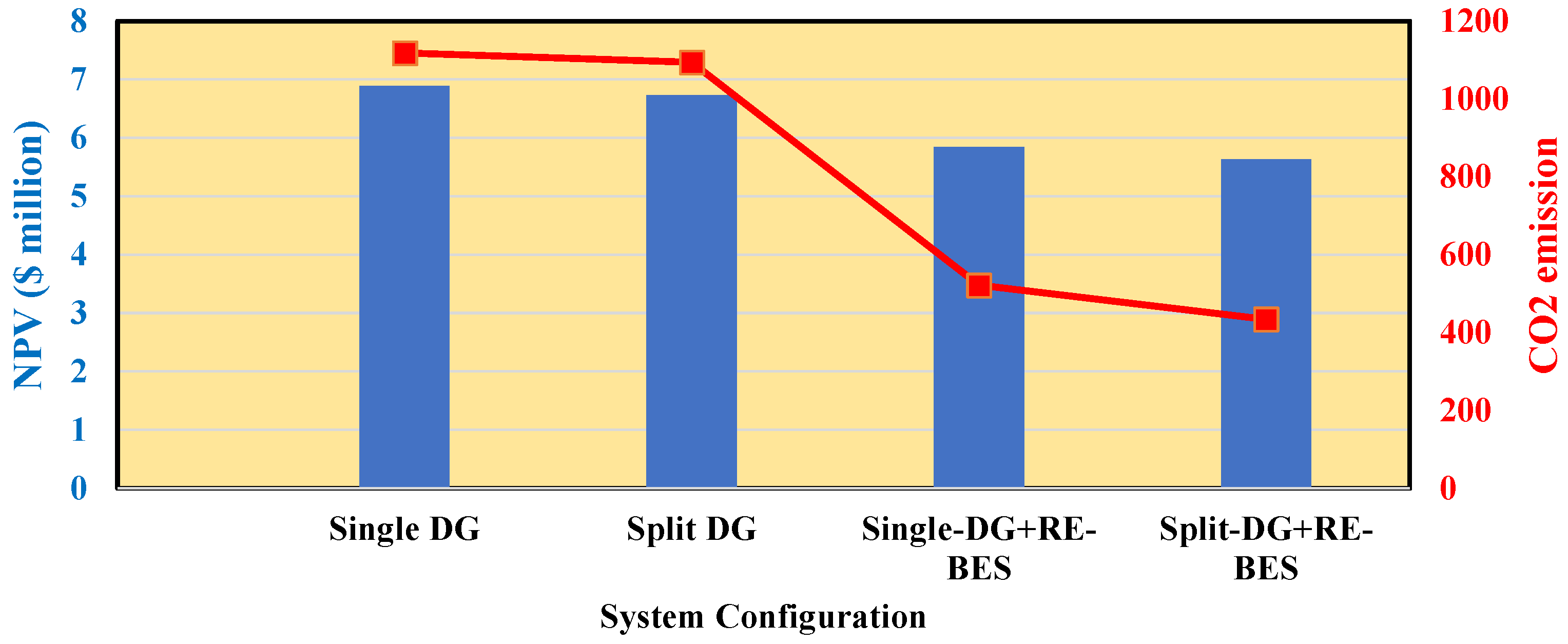
6.4. System Comparison

In this section, all three studied configurations are compared together and with two single-DG configurations (Single-DG and Single-DG-PV-WT-BES). The Single-DG configuration uses 100 kW DG and FT with the same storage capacity. The optimization results of the Single-DG configuration resulted in seven DGs and six FTs. For the Single-DG-PV-WT-BES configuration, 6 DGs, 41 WTs, 456 PVs, and 1312 BESs are obtained as the optimal results. Figure 15 compares the NPV and CO2 emission of all system configurations. As shown, the Split-DG-PV-WT-BES system has the lowest NPV and CO2 emission among the system configurations.

The comparison between Split-DG and Single-DG configurations shows that the Split-DG uses fewer litters of diesel than the Single-DG. This consumption reduction is due to decreased dumped energy, which is reduced around 30 MWh/year. This means that the Split-DG configuration has a better energy balance. Moreover, as expected, the CO₂ emissions decreased as well by 24 tonnes/year. The main difference between these two systems is that Split-DG has many small DGs that allows multiple configurations. This helps to follow the load variations easier as the DG1’s minimum output power is 10 kW. For instance, the minimum power delivered by the Single-DG model is 40 kW; thus, if the load in a time interval is 15 kW, then this DG will deliver an extra 25 kW that will be lost, contrary to Split-DG, where one DG1 can deliver that power without any excess. Therefore, from an economic point of view, the Split-DG system is better than the Single-DG. The reduction of diesel consumption mainly causes this difference in costs.

6.5. Advantages and Disadvantages

The proposed Split-DG with different sizes of DGs have some challenges, advantages, and disadvantages that should be discussed. The main advantage in comparison with the single size Split-DG is the flexibility of the proposed model to have different sizes. In the single size, all the small DGs should be selected to have the same size. If the size of the DG is large, then the dumped power is increased. On the other hand, if the single size is low, then the switching of the DGs would be a major problem. However, the proposed Split-DG uses a variety of sizes for the DGs that make it possible to better match with the load and, hence, the dumped power is decreased and there would be less switching between the DGs.

A major challenge with the Split-DG model is the switching between the DGs. It is true that the number of switching is lesser than that of the single size Split-DG, but still, there is a number of switching between the DGs in the proposed model. This switching should be on time with the load variations to ensure an uninterruptable power supply. On the other side, the switching may deteriorate the DGs operation and lifetime. The other challenge is the synchronization of the DGs in different sizes. It is true that generally, these small size DGs are available in the same voltage level, but their RPM may not be equal. Hence, extra devices may be needed for synchronization between the DGs.

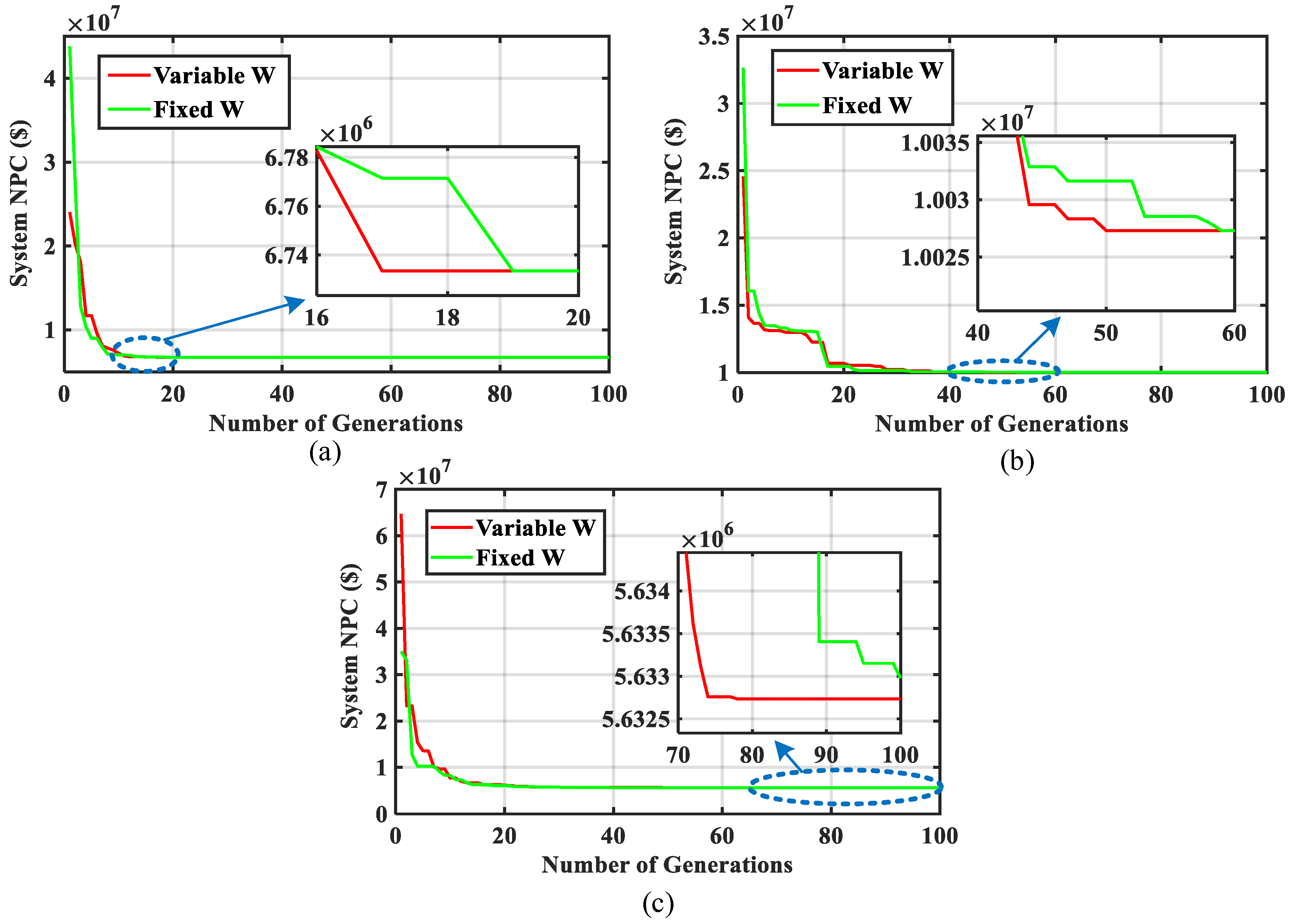
6.6. PSO Algorithm Comparison

This study compares the performance of the variable weighting factor PSO with the fixed weighting factor. In the variable weighting factor PSO, a gradual modification of the inertia weight index has been applied, which controls the movement of the particles in a direction. It is desired that the particle does not make substantial direction changes at the end of the iterative process to avoid a deviation during the convergency. Figure 16 illustrates the convergence rates of the PSO with variable and fixed weighting factors for all system configurations. In all three systems, PSO with variable weighting factor has reached the minimum NPV faster than the fixed one. Both algorithms converged to the same NPV in configurations 1 and 2. However, in configuration 3, which has more variables than the other systems, the fixed weighting factor PSO has not reached the minimum NPV in 100 generations.

7. Conclusions and Future Works

This paper optimized the capacity of Split-DG, WT, PV, and BES for a remote area community. The results of this study showed that the fuel cost has the largest portion of the NPV in the systems with DG. On the other hand, the battery cost has the largest portion of the NPV in the PV-WT-BES system. It was found that the interaction of different configurations of the Split-DG plays a crucial role in reducing fuel consumption, emissions, and dumped energy, and thus, reducing the total project’s cost compared to the conventional single-size DG systems. The Split-DG-PV-WT-BES system achieved the lowest NPV (AUD 5.6 million) and CO₂ emission (433.78 tonne/year). The NPV of the Split-DG-PV-WT-BES system was obtained almost AUD 1.1 million lower than that of the Split-DG system. The PV-WT-BES system was found to be unbelievably uneconomical, as its NPV was almost two times of the Split-DG-PV-WT-BES system. It was found that the proposed variable weighting factor PSO converged to the minimum NPV faster than the fixed weighting factor one. For configuration 3, the fixed weighting factor PSO could not reach the minimum NPV in 100 generations.

Future study may focus on the application of demand response in a system based on Split-DG, PV, WT, and BES. The demand response strategy could shift the loads in coordination with the switching between the small DGs in the Split-DG structure to decrease the fuel consumption and, hence, reduce the electricity cost and emission. Integration of hydrogen fuel cell in the considered microgrids is another direction for future works. Optimal sizing of the systems with fuel cell storage would be interesting to see the effect of the Split-DG on the size of fuel cell.

References

1. Renewable Energy/Off Grid. Available online: https://arena.gov.au/renewable-energy/off-grid/ (accessed on 25 September 2020).
2. Australia’s Off-Grid Clean Energy Market Research Paper. Available online: https://arena.gov.au/knowledge-bank/australias-off-grid-clean-energy-market-research-paper/ (accessed on 16 March 2021).
3. Babatunde, O.M.; Munda, J.L.; Hamam, Y. A Comprehensive State-of-the-Art Survey on Hybrid Renewable Energy System Operations and Planning. IEEE Access 2020, 8, 75313–75346. [Google Scholar] [CrossRef]
4. Bukar, A.L.; Tan, C.W. A review on stand-alone photovoltaic-wind energy system with fuel cell: System optimisation and energy management strategy. J. Clean. Prod. 2019, 221, 73–88. [Google Scholar] [CrossRef]
5. Maleki, A.; Pourfayaz, F. Optimal sizing of autonomous hybrid photovoltaic/wind/battery power system with LPSP technology by using evolutionary algorithms. Sol. Energy 2015, 115, 471–483. [Google Scholar] [CrossRef]
6. Zhang, G.; Shi, Y.; Maleki, A.; Rosen, M.A. Optimal location and size of a grid-independent solar/hydrogen system for rural areas using an efficient heuristic approach. Renew. Energy 2020, 156, 1203–1214. [Google Scholar] [CrossRef]
7. Moghaddam, M.J.H.; Kalam, A.; Nowdeh, S.A.; Ahmadi, A.; Babanezhad, M.; Saha, S. Optimal sizing and energy management of stand-alone hybrid photovoltaic/wind system based on hydrogen storage considering LOEE and LOLE reliability indices using flower pollination algorithm. Renew. Energy 2018, 135, 1412–1434. [Google Scholar] [CrossRef]
8. Fares, D.; Fathi, M.; Mekhilef, S. Performance evaluation of metaheuristic techniques for optimal sizing of a stand-alone hybrid PV/wind/battery system. Appl. Energy 2021, 305, 117823. [Google Scholar] [CrossRef]
9. Jurasz, J.; Ceran, B.; Orłowska, A. Component degradation in small-scale off-grid PV-battery systems operation in terms of reliability, environmental impact and economic performance. Sustain. Energy Technol. Assess. 2020, 38, 100647. [Google Scholar] [CrossRef]
10. Zahedi, A. Maximising solar PV energy penetration using energy storage technology. Renew. Sustain. Energy Rev. 2011, 15, 866–870. [Google Scholar] [CrossRef]
11. Dufo-López, R.; Bernal-Agustín, J.L.; Yusta, J.M.; Domínguez, J.A. Multi-objective optimisation minimising cost and life cycle emissions of stand-alone PV-wind-diesel systems with batteries storage. Appl. Energy 2011, 88, 4033–4041. [Google Scholar] [CrossRef]
12. Combe, M.; Mahmoudi, A.; Haque, M.H.; Khezri, R. AC-coupled hybrid power system optimisation for an Australian remote community. Int. Trans. Electr. Energy Syst. 2020, 30, e12503. [Google Scholar] [CrossRef]
13. Gebrehiwot, K.; Mondal, M.A.H.; Ringler, C.; Gebremeskel, A.G. Optimisation and cost-benefit assessment of hybrid power systems for off-grid rural electrification in Ethiopia. Energy 2019, 177, 234–246. [Google Scholar] [CrossRef]
14. Ogunjuyigbe, A.S.O.; Ayodele, T.R.; Akinola, O.A. Optimal allocation and sizing of PV/Wind/Split-diesel/Battery hybrid energy system for minimising life cycle cost, carbon emission and dump energy of remote residential building. Appl. Energy 2016, 171, 153–171. [Google Scholar] [CrossRef]
15. Khezzane, K.; Doumbia, M.L.; Khoucha, F. Multi-objective Sizing of Hybrid Generation Energy System for Remote Area Using Genetic Algorithm. In Proceedings of the 2021 Sixteenth International Conference on Ecological Vehicles and Renewable Energies (EVER), Monte-Carlo, Monaco, 5–7 May 2021; pp. 1–9. [Google Scholar] [CrossRef]
16. Asefi, S.; Shayeghi, H.; Shahryari, E.; Dadkhah, R. Optimal management of renewable energy sources considering split-diesel and dump energy. Int. J. Tech. Phys. Probl. Eng. 2018, 10, 34–40. [Google Scholar]
17. Mohammed, A.Q.; Al-Anbarri, K.A.; Hannun, R.M. Optimal Combination and Sizing of a Stand-Alone Hybrid Energy System Using a Nomadic People Optimizer. IEEE Access 2020, 8, 200518–200540. [Google Scholar] [CrossRef]
18. Ayodele, T.R.; Ogunjuyigbe, A.S.O.; Akinola, O.A. N-split generator model: An approach to reducing fuel consumption, LCC, CO2 emission and dump energy in a captive power environment. Sustain. Prod. Consum. 2017, 12, 193–205. [Google Scholar] [CrossRef]
19. Mohandes, B.; Acharya, S.; El Moursi, M.S.; Al-Sumaiti, A.S.; Doukas, H.; Sgouridis, S. Optimal Design of an Islanded Microgrid With Load Shifting Mechanism Between Electrical and Thermal Energy Storage Systems. IEEE Trans. Power Syst. 2020, 35, 2642–2657. [Google Scholar] [CrossRef]
20. Sources of Greenhouse Gas Emissions. Available online: https://www.epa.gov/ghgemissions/sources-greenhouse-gas-emissions. (accessed on 3 February 2022).
21. Analysis of 10-year record. Available online: http://www.renewablessa.sa.gov.au/topic/investor-information/renewable-energy-resource-maps/solar-energy-resource-maps (accessed on 11 October 2021).
22. About the Renewable Energy. Available online: http://www.cleanenergyregulator.gov.au/RET/About-the-Renewable-Energy-Target (accessed on 12 October 2021).
23. AlRashidi, M.R.; Alhajri, M.F.; Al-Othman, A.K.; El-Naggar, K.M. Particle Swarm Optimization and Its Applications in Power Systems. In Computational Intelligence in Power Engineering; Panigrahi, B.K., Abraham, A., Das, S., Eds.; Springer: Berlin, Germany, 2010; pp. 295–324. [Google Scholar] [CrossRef]
24. Mazhoud, I.; Hadj-Hamou, K.; Bigeon, J.; Joyeux, P. Particle swarm optimisation for solving engineering problems: A new constraint-handling mechanism. Eng. Appl. Artif. Intell. 2013, 26, 1263–1273. [Google Scholar] [CrossRef]
25. Population. Available online: https://plan.sa.gov.au/state_snapshot/population#:~:text=in%20South%20Australia,Population%20change%20in%20South%20Australia,average%20of%2010%2C300%20per%20year (accessed on 7 August 2021).
26. Climate data online. Available online: http://www.bom.gov.au/climate/data/index.shtml?bookmark=200 (accessed on 14 October 2021).
Figure 1. Single-line diagram of the proposed remote microgrid.
Sustainability 14 02892 g001
Figure 2. Diesel generators control in a Split-DG system.
Sustainability 14 02892 g002
Figure 3. Example of the distribution of the load power in the Split-DG system.
Sustainability 14 02892 g003
Figure 4. Flowchart of PSO with variable weighting factor.
Sustainability 14 02892 g004
Figure 5. System input data, (a) daily energy demand, (b) daily solar insolation, (c) daily average wind speed, and (d) daily average ambient temperature.
Sustainability 14 02892 g005
Figure 6. NPV fraction of the optimized solution for Configuration 1.
Sustainability 14 02892 g006
Figure 7. Annual operation of Configuration 1. (a) Total diesel generation and (b) dumped power.
Sustainability 14 02892 g007
Figure 8. The 48-h operation of Configuration 1: (a) generation and demand and (b) online DGs.
Sustainability 14 02892 g008
Figure 9. NPV fraction of the optimized solution for Configuration 2.
Sustainability 14 02892 g009
Figure 10. Annual operation of Configuration 2. (a) Total RE generation, (b) SOC, and (c) power dumped.
Sustainability 14 02892 g010
Figure 11. The 48-h operation of Configuration 2: (a) generation and demand and (b) BES’s charge and discharge.
Sustainability 14 02892 g011
Figure 12. NPV fraction of the optimized solution for Configuration 3.
Sustainability 14 02892 g012
Figure 13. Annual operation of Configuration 3. (a) Total RE generation, (b) total DG generation, (c) SOC, and (d) power dumped.
Sustainability 14 02892 g013
Figure 14. The 48-h operation of Configuration 3: (a) generation and demand and (b) BES’s charge and discharge.
Sustainability 14 02892 g014
Figure 15. NPV and CO2 comparison of all system configurations.
Sustainability 14 02892 g015
Figure 16. Convergence rate comparison of the PSO with variable and fixed weighting factors: (a) Configuration 1, (b) Configuration 2, (c) Configuration 3.
Sustainability 14 02892 g016